Investigating the Impact of Accessibility on Internal Migration Flows in Italy Through the Calibration of Multiple Linear Regression Models

Abstract

This study estimates the impact of some socio-economic, real estate, and accessibility factors on the demographic change of the Italian provinces. Migration rates were analysed for one hundred and thirteen provincial capitals, or former provincial capitals, and their territories, and the correlation between them and various socio-economic and accessibility variables was studied. The data analysis showed significant heterogeneity between the different territorial areas of the country, highlighting the well-known phenomenon of migration from southern to northern regions. The aim of this paper is to investigate whether and to what extent accessibility variables have a direct influence on internal migration phenomena, in addition to the other socio-economic variables involved. Multiple linear regression models were specified and calibrated to correlate migration rates with various socio-economic and accessibility variables. The results show a non-negligible impact of certain accessibility variables on the migration phenomenon and suggest the need to work on the infrastructure front to rebalance the country’s demographic and socio-economic structure.

1. Introduction

The demographic decrease in Europe is a well-known, widely studied, and constantly evolving phenomenon. The European Union has set up a standing committee of 43 MEPs called the Committee on Regional Development (REGI), which is responsible, among other things, for implementing and improving the Union’s regional development and cohesion policy according to the EU Treaties. Based on the report produced by this commission in 2021 [1], the European Parliament considered the combination of migration flows and low birth rate to be decisive in the depopulation of some regions, especially in Eastern and Southern Europe. Furthermore, it identified several critical issues caused by this phenomenon, including the so-called ‘brain drain’, i.e., the impoverishment of highly skilled and qualified personnel, deficits in the provision of health and cultural services, information technology, and physical connectivity, particularly in terms of transport, education, and employment opportunities. Among other things, the transport system was identified as a possible lever to counter this phenomenon, and the inclusion of specific actions for rural and peripheral regions would also be a step towards solving the problem: “The EU should not neglect the rural and remote regions in its mobility strategy: transport networks can halt depopulation by reinforcing rural-urban connectivity” [2].

Regarding Italy, the subject of this work, the ISTAT 2023 report [3] identified a decrease in emigration and an increase in internal mobility and immigration. In particular, the regions of Southern Italy suffered a demographic decline of 525,000 inhabitants between 2012 and 2021.

The reasons for this phenomenon are complex and heterogeneous, and their identification is not easy since there are several factors involved. Although the phenomenon has been studied from different points of view, the socio-economic conditions, the availability of services, and job opportunities as the main factors favouring internal migration from the most depressed areas to the richest ones of a country have not been considered in previous studies. To the best of our knowledge, a specific study on the influence that accessibility may have on this phenomenon in the Italian context is not yet available in the literature. This study aims to fill this research gap.

Therefore, the aim of this study is to investigate the correlation between changes in the total migration rate (to and from other Italian provinces and to and from abroad) and accessibility, trying to find correlated variables and to identify a possible causal relationship. Verifying how and in what way some accessibility variables influence the migration rate and being able to quantify the effect of interventions on transport systems from this point of view can guide transport planning and policy, as well as taking into account these effects, which have a social, as well as economic, impact that is relevant for the organic and inclusive development of the country.

Over 180 linear regression models were calibrated by setting the total migration rate as a function of various accessibility and socio-economic variables. The models were calibrated using demographic data from 2017 to 2022 for 105 Italian provinces.

Since these data are usually available, the proposed methodology is applicable to any territory in the world. It is also applicable to superordinate territorial units, such as regions and nations, and to subordinate territorial units, such as municipalities.

The main limitation of the proposed methodology is that it cannot examine migration flows within a territorial unit; this aspect of the problem can be dealt with in further research developments.

This document is structured as follows. Section 2 examines the background. Section 3 defines the variables and data used. Section 4 describes the specification and calibration of the regression models. Section 5 discusses the results. Finally, Section 6 summarises the conclusions. Appendix A reports the data used.

2. Background

Italy is a southern European nation with a population of about 59 million and a territory of about 302,000 square kilometres; the average population density is about 195 inhabitants/km². The per capita GDP is about EUR 33,000 per inhabitant [4], with substantial disparities between different areas of the country: the regions of Northern Italy have an average per capita GDP of about EUR 40,000, which is reduced to about EUR 35,000 for the regions of Central Italy and reaches about EUR 22,000 for the regions of Southern Italy and the islands. This economic disparity, which is also representative of a different labour market, is one of the causes of internal migration that this study deals with.

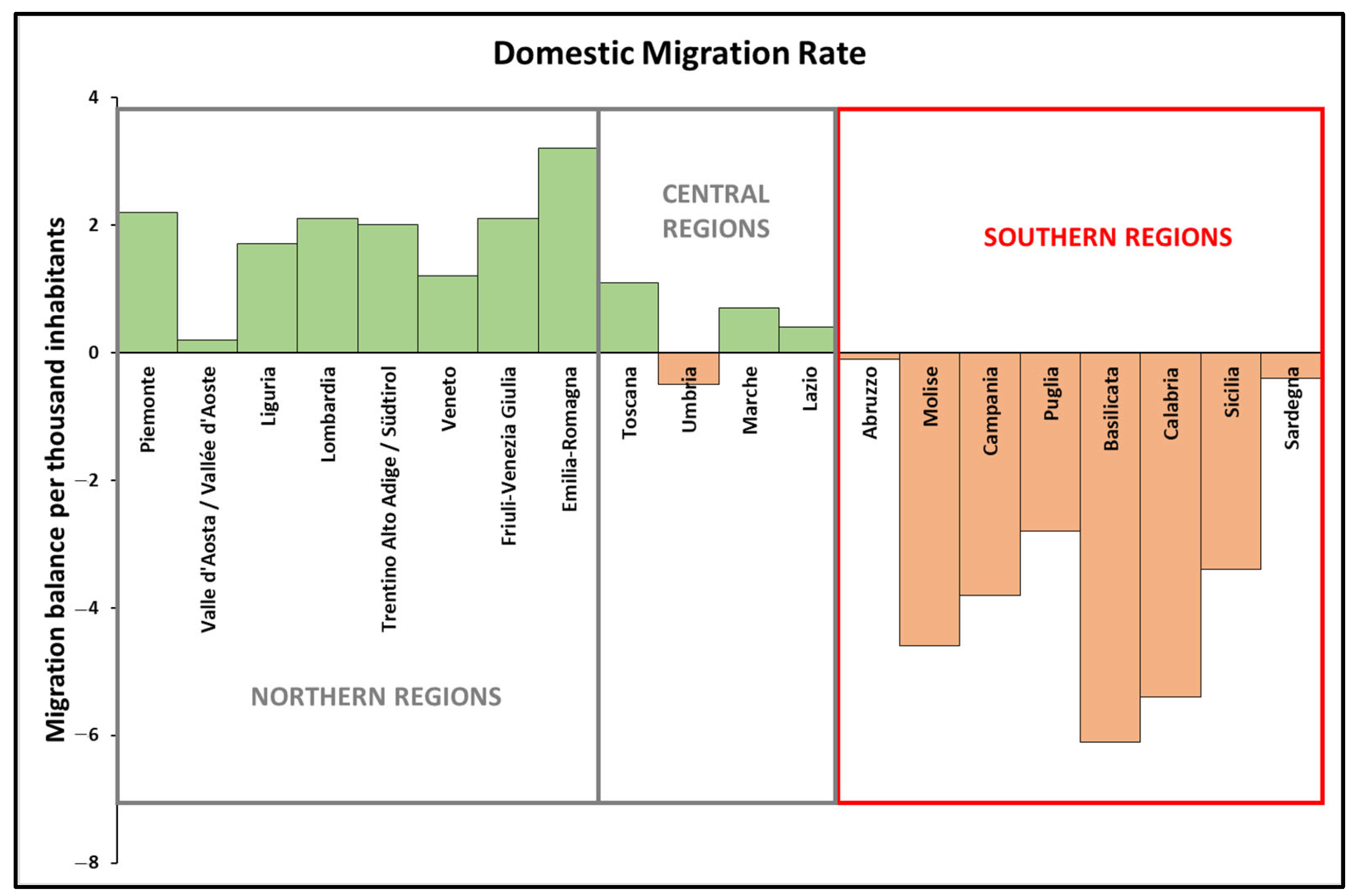
Statistical data [4,5] show that in 2023, there were about 1.44 million changes in residence (see Figure 1), in line with the growing trend of the last decade.

Southern Italy records an outflow of inhabitants that is not compensated for by a corresponding inflow: in 2023, internal outward migration from the southern regions was about 407,000, while incoming migration was about 344,000, with a net loss of 63,000 inhabitants. The migration rate in these regions is −3.2 per thousand inhabitants. Northern Italian regions, on the contrary, are more attractive: transfers to a Northern Italian municipality from any other municipality amounted to about 842 thousand, of which 785 thousand came from another northern municipality, with a migration rate of +2.1 per thousand inhabitants.

International migratory flows show about 416 thousand entries and a growth of +1.1% compared to the previous year. On the contrary, outgoing migration from Italy to other countries is strongly decreasing: −5.6% compared to 2022 and −21% compared to 2019.

An additional data analysis [4] highlights an increase in internal migration, while outgoing international migration is still in line with pre-COVID-19 pandemic data. The restrictions of the pandemic have strongly influenced international inbound migration: after an all-time peak of 301,000 entries in 2017, Italy recorded a drop of 192,000 foreign entries in 2020 and 244,000 in 2021. In 2022, there were 336,000 entries; in 2023, they reached 360,000, setting new records for immigration from abroad. Based on these data, it can be said with certainty that COVID-19, while having impacted international inbound migration, did not negatively affect internal migration, which actually increased.

Migration to some territories at the detriment of others is a phenomenon that can cause socio-economic imbalances with an inefficient spatial distribution of resources.

The phenomenon of migration has been widely studied in the literature, with different methodological and theoretical approaches. Many studies have dealt with international migration, for which several theories have been proposed. A review and analysis of the theories of global migration can be found in [6,7,8]. The main theories are (i) the neoclassical theory, (ii) the new economics theory, (iii) the world systems theory, and (iv) the dual labour market theory.

The neoclassical theory [9] hypothesises that migration is determined by the differences between the returns on labour in different markets, particularly salary differences, and the different supply and demand for labour. In addition to a macro approach, i.e., based on aggregate data, it is possible to simulate individual choice at a micro level with the human capital theory of migration [10].

The new economics theory [11] hypothesises that the decision to migrate is not made by a single person but by entire families, taking into account not only income factors but also the difference in the family’s income compared to other families and the risk aversion of sending a family member abroad. This theory is usually considered less solid and less frequently used than others, due to the difficulty of evaluating some variables involved that would be necessary for its implementation.

The world systems theory [12] considers that the migratory phenomenon is influenced by structural changes in world markets, globalisation, the interdependence between economies, and innovative forms of production. Therefore, capital mobility is seen as interconnected to the mobility of people for work reasons. The theory also takes into account global political and economic inequalities.

The dual labour market theory [13] hypothesises that migration is mainly influenced by the demand for labour, distinguishing between capital-intensive economies, where both skilled and unskilled labour are required, and labour-intensive economies, where the primary demand is for unskilled labour. This theory cannot explain the different immigration rates in countries with similar types of economies.

Internal migration within a country has also been studied; the phenomenon differs for developing countries [14] and developed countries [15].

In the first case, the search for a job is one of the main factors that leads to internal migration; the attractiveness of areas depends on the presence of industrial activities, salary differences, and employment levels. Furthermore, the presence of a network, i.e., relatives or friends in a specific area, has an additional attractive effect, also due to the availability and ease of obtaining information on job opportunities. In the second case, migration allows the workforce to be redistributed geographically according to economic and demographic changes and differences. The human capital model is a valuable tool for studying labour economics, but it is not sufficient to explain the phenomenon of internal migration on its own.

One study [16] focused on the Italian case study and used a gravitational model to study internal migration based on human capital, considering per capita GDP, unemployment rate, population, and level of education as variables—the work identified per capita GDP and the unemployment rate as the main variables influencing migratory flows.

Some classic migration theories were tested in [17], highlighting how it would be useful to develop more complex models to interpret the phenomenon, considering that some theories, when verified on real data, fail to reproduce them accurately.

Internal migration is influenced by the same variables that generate international migration. The objective of this work is to verify if and to what extent the accessibility of the territories and the available transportation services, with reference to high-speed rail, influence internal migratory choices. Transport infrastructures and services generate economic and spatial impacts [18]; among the spatial impacts, those on accessibility are particularly relevant, influencing regional development in the European Union [19].

The importance of infrastructure and transportation services for the socio-economic development of a territory or a community has been widely studied in the literature.

The effect that an inefficient distribution of high-speed rail (HRS) services can have on certain territories was recently studied in [20]. It was found that opening new high-speed stations can reduce migration not only in the cities directly involved but also in neighbouring territories. It has been shown [21] that implementing a high-speed rail network can produce economic growth in urban areas with appreciable effects over five years. According to a Chinese study [22], a reduction in the resident population can be aggravated by improper planning of motorway and high-speed rail infrastructure, particularly for cities that are affected by demographic and economic shrinking. Another study in China [23] focused on the impact of HSR services on the development of the industrial structure of some of the country’s non-central cities; the positive effects were mainly shown for cities less than 100 km away from a central city (provincial capital or city controlled by the central government). Kim [24] examined, for a case study in Korea, the impact of the development of the high-speed railway between Seoul and Pusan on changes in the spatial structure in the region, finding a trend towards population concentration in the area around the capital.

Since the effects of high-speed railways on the labour market have been little studied in previous decades, some recent efforts have been made, such as the calibration of a linear regression model limited to the Madrid metropolitan area [25], which shows that while the growth of labour contracts has increased thanks to high-speed rail services, the unemployment rate and house prices became increasingly less significant in the reference period (2004–2015). Furthermore, the greater accessibility enabled by the introduction of high-speed rail increased interregional economic connections, which also included the labour force, and interregional economic models shifted from a point–axis model to a network model [26].

The economic impacts, in terms of interregional disparity and territorial distribution, produced by introducing a large-scale HSR system were estimated by combining industrial input–output relations with changes in passenger accessibility [27].

Road infrastructure can also have an important socio-economic impact in some rural areas. A study in China [28] showed that improving road infrastructure impacts the income of rural residents; this impact was more significant for those who initially had lower incomes.

A study in the United States [29] showed how restrictive housing policies can contribute to the decline in growth by generating a phenomenon of spatial deallocation.

Regarding inter-urban migration phenomena in large cities and other urban planning and transport aspects, urban ‘sprawl’ and the accessibility of transport to urban centres have been identified as causes of migration to large cities in Russia [30]. The impact of international immigration on the unemployment rate in Canada has been studied in [31], showing that in the short term, there is an increase in the number of people unemployed due to the difficulty of integration, but in the long term, this effect is reabsorbed. The link between migration and employment rates in the United Kingdom has been studied in [32]. A study of the impact of migration on Asian countries is reported in [33].

The accessibility and availability of transport infrastructure and services significantly impact property values [34,35,36,37], highlighting the importance of analysing all externalities, positive and negative, of transport investments.

The effects of the correlation between infrastructure development and the property market have been studied in China [38]; in particular, the increase in housing prices went hand in hand with the rise in the demand and the introduction of transit systems, such as trams [39], even if these studies are limited to a restricted territorial area.

Demographic imbalances in Italy are commonly recognised, and the resulting inequalities are considered very impactful and predominantly linked to socio-economic variables [40]. A study of forty years of data on Italian migration has shown that individual characteristics such as sex, age, and skills have an impact on the weight of economic factors [41]. A recent study on Italian demographic vibrancy [42] included accessibility as an index based on travel time and concluded that the introduction of high-speed rail services alone is not able to change demographic trends, even though it influences the dynamics of some demographic indices by attracting weaker demographic classes to more accessible locations.

3. Data and Methods

The data collection and analysis phase encountered difficulties due to the heterogeneity of the different sources, which sometimes referred to different periods. Demographic data and some socio-economic data were taken from ISTAT (National Institute of Statistics), income data from the MEF (Ministry of the Economy and Finance), data on property values from the Italian Fiscal Agency, data on university locations and personnel from the MUR (Ministry of Universities and Research), and, finally, accessibility data were calculated using specifically implemented models.

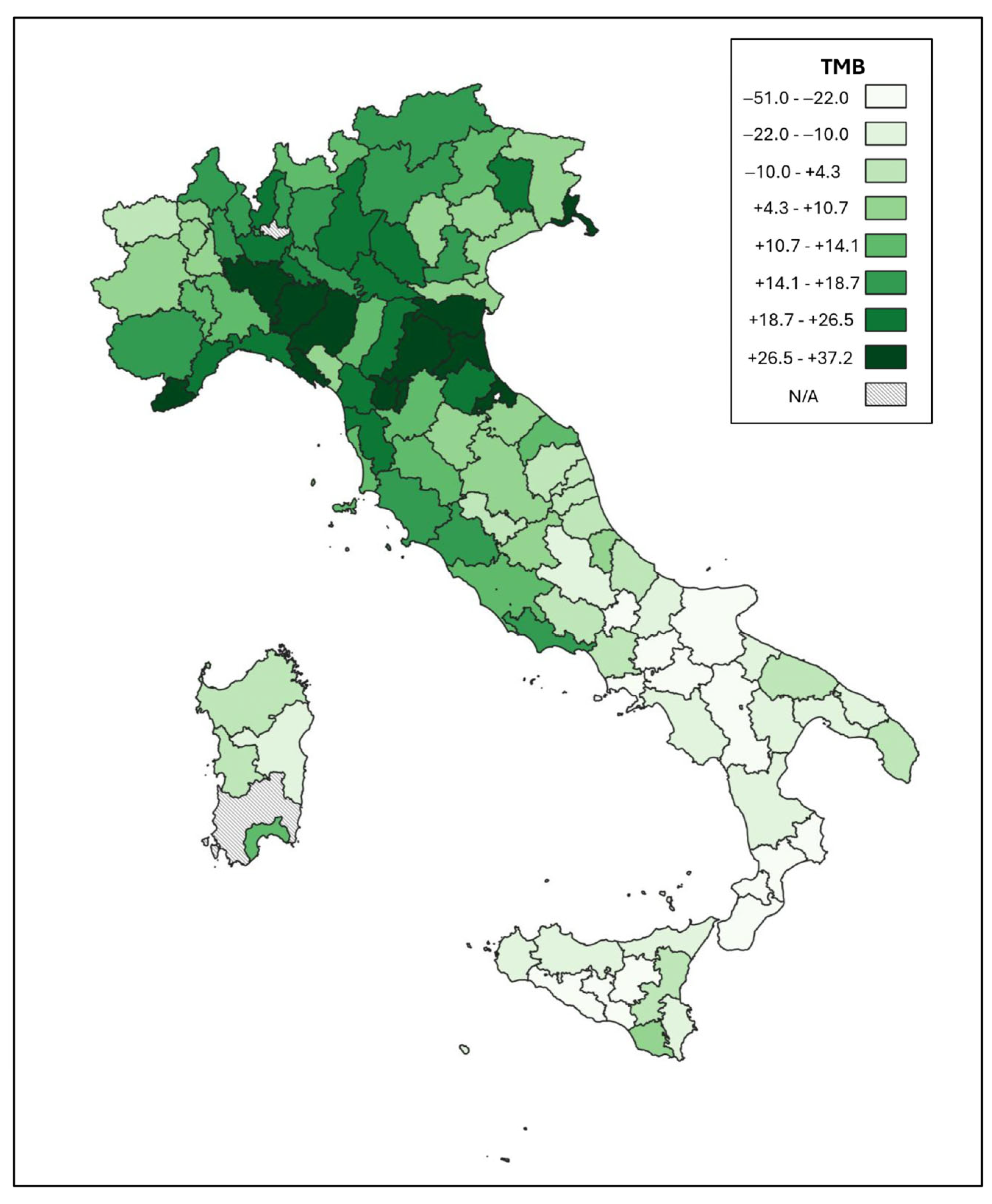
The database has the province as its basic territorial unit; where necessary, data were derived from the municipalities composing each province. Since the study needed to be based on the variation over the years of the characteristics of the territories, and the migration rate refers to a specific time interval, in some cases, it was necessary to combine or separate the territorial units. Indeed, during the reference period, some provinces were merged or separated; therefore, the data for these provinces were not homogeneous. Where it was possible to correct the data, they were homogenised and maintained in the database (6 provinces), while, in other cases, removing them from the database was necessary. Overall, only 2 provinces of 107 were removed from the database for these reasons; the provinces not considered are highlighted in Figure 2 with a dotted background (N/A) and are ‘Monza e Brianza’ and ‘Sud Sardegna’.

This study analysed the total migration balance between 2017 and 2022; in the following sections, this variable takes on the role of the dependent variable, representing the phenomenon we want to explain according to the available data. The generic territory (in our case, the generic province) is denoted by i, and the total migration balance is denoted by tmb_i. This variable is equal to the sum of the annual migration balance for 2017 to 2022; the yearly migration balance is the difference between the number of registrations and the number of cancellations from the population registers. 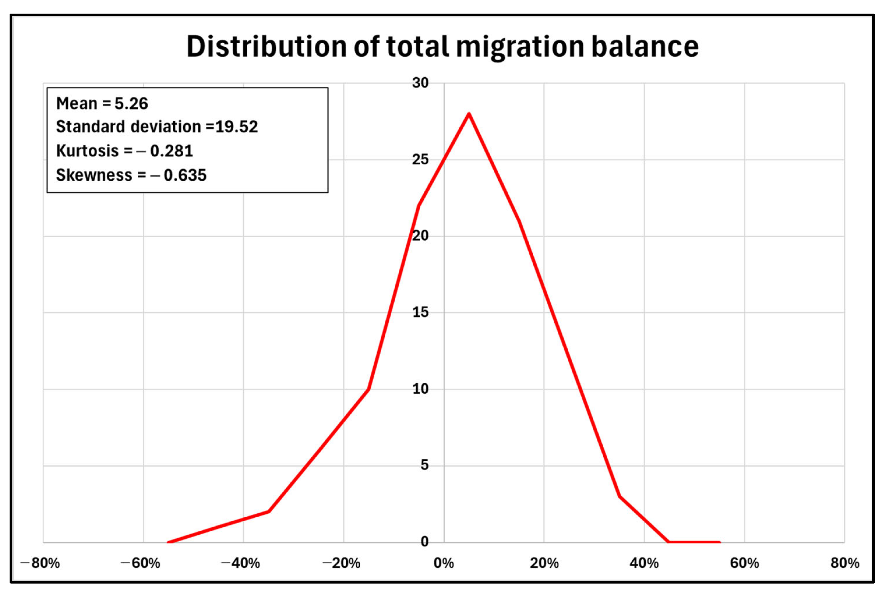It is then related to the number of inhabitants of each territorial unit so that it is expressed in percentage terms and, more precisely, as per thousand (⁰/₀₀). The values of this indicator were calculated based on registry data provided by ISTAT; their distribution is shown in Figure 3, while Figure 2 shows the different values on a map. It should be noted that, as the calculation was based on registry data, the migratory balance also includes data on legal immigrants moving from one region of the country to another. Given the study’s primary objective, which is to assess the impact of accessibility, this is not considered to have altered the phenomenon analysed. The period analysed includes the COVID-19 pandemic, during which the migratory phenomenon was limited, if not absent. To limit the impact of this disturbance on the data, an extended period (5 years) was used, and the data were the sum of the annual migratory balances, which led to an estimate of the overall variation, not an average value, of the population in the 5 years. Considering that the objective of the analysis was to evaluate the impact of accessibility on the phenomenon, it is believed that the approach used can be regarded as valid for this specific study.

The explanatory variables, i.e., those able to explain the phenomenon of internal migration flow, are described in the following subsections and classified into:

• Socio-economic variables;
• Property value variables;
• Accessibility variables.

The choice of variables was based on the analysis of the literature and the authors’ experience in the sector.

The socio-economic variables considered refer mainly to three factors: (1) aspects related to the labour market (employment/unemployment rate and number of job holders); (2) aspects related to the economic wealth of the territory (average income); and (3) the presence or absence of a university. Except for the variable under point (3), which was included to verify whether the presence or absence of a university could have a significant influence on the phenomenon of migration, the other variables represent the main factors influencing internal migration in Western countries, as can be seen from the analysis of the literature and documents produced by the European Union. For international migration, other factors must be considered alongside the economic ones, from wars to climate change, which are clearly not considered in this case. The choice for the real estate values was the variable usually used in similar studies [34]. For the accessibility variables, those most frequently used in studies concerning other phenomena in which accessibility plays an important role were chosen [43,44].

The values of all variables tested, both those taken from public databases and those generated by the transport supply model or calculated by us, are reported in Appendix A so as to allow the reproducibility of the results obtained.

3.1. Socio-Economic Variables

The socio-economic variables, calculated by provincial territory, refer to the employment rate, the number of employed persons classified by sector of activity, and the variables for the presence or absence of a university. These variables and their description are given below:

• or_i, occupation rate, calculated as the ratio of employed persons to the population aged 15 years or over;
• ur_i, unemployment rate, calculated as the ratio of persons seeking jobs to the labour force, where the latter includes employed and unemployed persons;
• aipc_i, average income per capita, calculated by dividing the total taxable income by the number of inhabitants;
• jh_i, job holders per inhabitant, calculated as the ratio of the number of job holders to the population;
• mjh_i, job holders in manufacturing activities per inhabitant;
• cjh_i, job holders in commercial activities per inhabitant;
• ejh_i, job holders in educational activities per inhabitant;
• ajh_i, job holders in all other activities per inhabitant;
• ujh_i, job holders in university teaching and research activities per inhabitant;
• uni_i, presence of a university, dummy variable (0/1).

3.2. Property Value Variables

Property values can also impact migration phenomena, although the influence is uncertain: high values may indicate a good quality of life, thus attracting people, but can also be an obstacle for lower incomes. In this work, the following variable was considered:

• apv_i, an average of residential property values by provincial territory. The median between the minimum and maximum residential property values, in euros per square metre, for municipalities j in each province i was calculated based on the values provided by the Italian Fiscal Agency. Of these values, the average for each province i was calculated:

  $$a{pv}_i=\left({\sum }_{j\in prov\_i}{\displaystyle \frac{{Vmin}_j-{Vmax}_j}{2}}\right)/n_i\hspace{1em} {\forall }_i\hspace{1em}[€/{\mathrm{m}}^2]$$

  where
  prov_i is the set of municipalities belonging to province i;
  Vmin_j [Vmax_j] is the minimum [maximum] property value per square metre in municipality j;
  n_i is the number of municipalities within province i.

3.3. Accessibility Variables

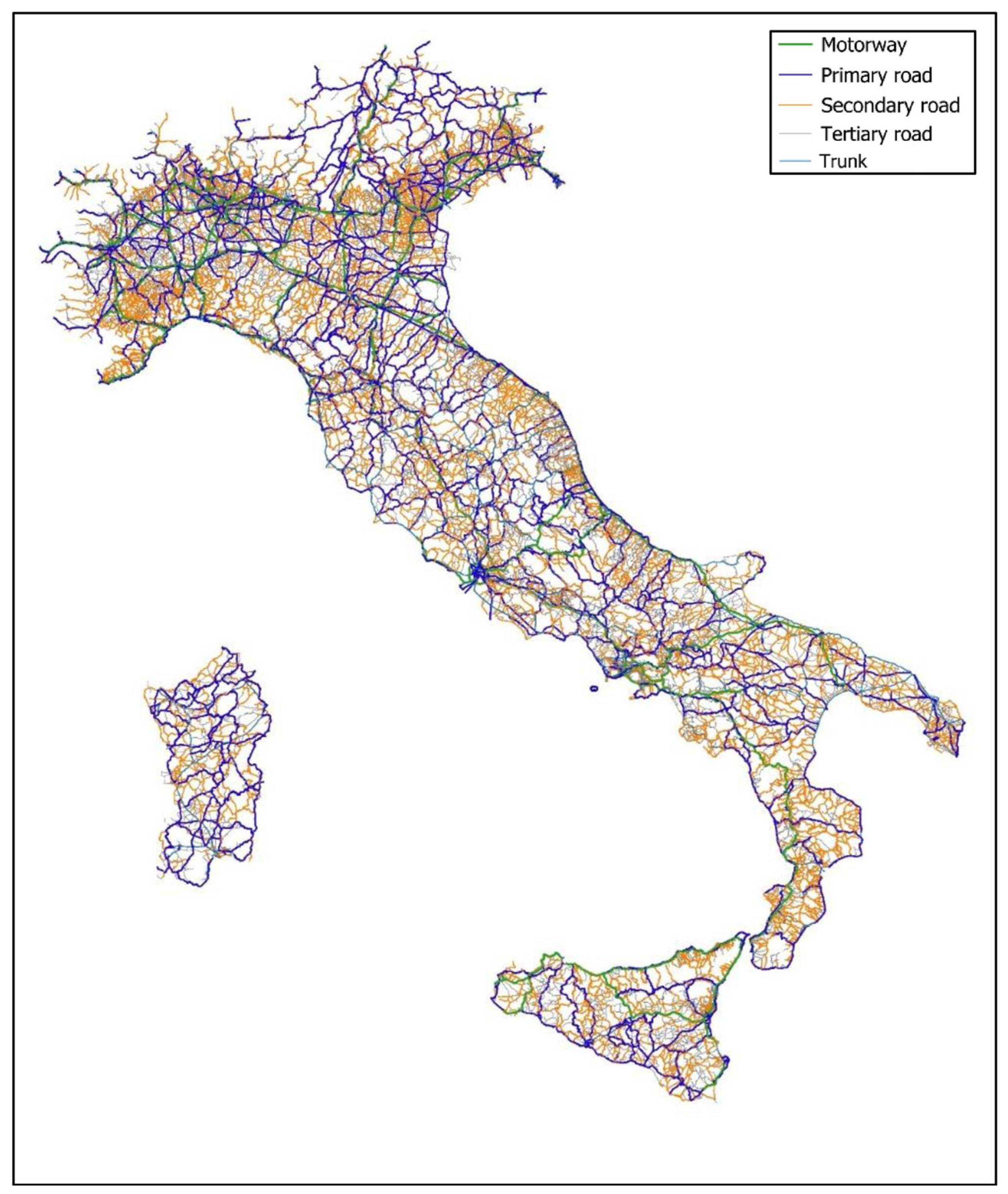
The accessibility variables were calculated using a method similar to that proposed in [43]. The calculation of some of these variables required the construction of a road transport supply model. This model was developed in previous research, and the paper was just cited. Figure 4 shows the graph of the road network, which consists of 767,674 links and represents 202,628 km of road (more details are given in [43]).

The following subsections describe the different accessibility variables proposed.

3.3.1. Availability of High-Speed Rail Services

It measures the presence of high-speed rail services. The variable, expressed as hsr_i, reports the number of runs on high-speed railway lines arriving at/departing from the station of the provincial capital. If the service is absent, the value of this variable is zero.

3.3.2. Distance from Rome Leonardo da Vinci Airport

The Rome Leonardo da Vinci Airport is Italy’s largest and most important hub. Most intercontinental and international connections depart from and arrive at this airport. Therefore, it is considered that greater or lesser proximity may affect migration. The proposed variable, dha_i, is the reciprocal of the distance between the provincial capital and the airport site, measured on the road graph described above:

$${dha}_i=1/{dist\_ha}_i\hspace{1em} {\forall }_i$$

where dist_ha_i is the distance between province capital i and Leonardo Da Vinci airport (hundreds of km).

3.3.3. Distance from the Nearest International Airport

A variable similar to the previous one refers to the nearest international airport. In each region, only the international airport with the most passengers served was considered in case the region hosted more than one airport. The list of international airports considered is shown in

Table A4. International airports.

Region	Airport	Municipality
Piemonte	Turin–Caselle	Caselle Torinese
Aosta Valley	N/A	N/A
Lombardy	Milan–Malpensa	Ferno
Trentino–Alto Adige	Bolzano	Bolzano
Veneto	Venice–Tessera	Venice
Friuli–Venezia Giulia	Trieste–Ronchi dei Legionari	Ronchi dei Legionari
Liguria	Genoa–Sestri	Genoa
Emilia-Romagna	Bologna–Borgo Panigale	Bologna
Tuscany	Pisa–San Giusto	Pisa
Umbria	Perugia	Perugia
Marche	Ancona–Falconara	Falconara Marittima
Lazio	Rome–Fiumicino	Fiumicino
Abruzzo	Pescara	Pescara
Molise	N/A	N/A
Campania	Naples–Capodichino	Naples
Apulia	Bari–Palese	Bari
Basilicata	N/A	N/A
Calabria	Lamezia Terme	Lamezia Terme
Sicily	Catania–Fontanarossa	Catania
Piemonte	Turin–Caselle	Caselle Torinese
Sardinia	Cagliari–Elmas	Elmas

in Appendix A.

The variable, dia_i, is calculated as the reciprocal of the distance of the provincial capital from the nearest airport:

$${dia}_i=1/{{min}_k(dist\_ia}_{i,k})\hspace{1em}\hspace{1em}{\forall }_i$$

where

k indicates the generic international airport;

dist_ia_i,k is the distance between province capital i and the international airport k (hundreds of km).

3.3.4. Population-Weighted Road Accessibility

Another aspect that is supposed to be relevant to the migration phenomenon is road accessibility. This type of accessibility can be calculated in several ways; in this work, the calculation was carried out using the gravity-based method proposed by Hansen [45], which was adequately adapted to the purposes of the analysis.

For each province, i, the variable, denoted ra_i, was calculated as

$${ra}_i={\sum }_{m\ne i}{inh}_m/{rt}_{i,m}\hspace{1em}\hspace{1em}{\forall }_i$$

where

m indicates a generic municipality other than i;

inh_m indicates the number of inhabitants in the municipality m;

rt_i,m is the travel time by car between locations i and m, calculated using the supply model described above.

3.3.5. Road Distance Indicator

Another indicator of accessibility, rd_i, is based on the distance within the road network (in km × 10⁻³) between provincial capital i and any other municipality, m. We calculate this indicator as follows:

$${rd}_i=1/{\sum }_{m\ne i}{d}_{i,m}\hspace{1em}\hspace{1em}{\forall }_i$$

where d_i,m represents the distance between provincial capital i and municipality m.

3.3.6. Road Travel Time Indicator

This indicator, denoted by rtt_i, is similar to the previous one, only it is based on car travel time, calculated using the transport supply model described above:

$${rtt}_i=1/{\sum }_{m\ne i}{rt}_{i,m}\hspace{1em}\hspace{1em}{\forall }_i$$

where rt_i,m has already been defined above.

4. Regression Models

The objective of this study was to calibrate a model that is able to estimate the influence that the variables defined above may have on migratory phenomena. Even if the main focus is on accessibility, it is necessary to consider all the variables that are considered useful in explaining the phenomenon so as to be able to weigh the contribution of each variable correctly. To formulate a model that best represents the contribution of each variable, it is necessary to test multiple combinations of them, thus calibrating multiple models and choosing the one that best approximates the reality.

Among the different possible models, we chose to use multiple linear regression models [46], which have strengths and weaknesses. Among the strengths, the main ones refer to the speed with which they can be calibrated (practically, in closed form and many software programs, including Excel, have tools for their calibration), to the many who have used them in different scientific sectors, and to the ease of generating reliable statistical tests to evaluate the goodness of the model. The main weak point is the hypothesis that the studied phenomenon has a linear relationship with each explanatory variable.

More complex models, such as spatial econometric models [47] or machine learning techniques [48], can interpret migratory phenomena by considering other variables, such as cultural ties, language, prevailing religion, and government structures, which can influence some migratory decisions. In this study, we considered it sufficient to use a multiple linear regression model, both because the primary purpose was to evaluate the impact of accessibility variables and because, when dealing with internal migration, the aforementioned variables have a less significant impact than in the case of international migration.

A multiple linear regression model relates a dependent variable, Y, with several independent variables, X; a general formulation can be expressed as

$$Y={\beta }_0+{\beta }_1{X}_1+{\beta }_2{X}_2+\cdots +{\beta }_n{X}_n$$

where the β terms represent the coefficients of the model to be calibrated.

The linear regression model must be ‘specified’ and ‘calibrated’. The specification phase defines the variables to be present in the model, while the calibration phase defines the values assumed by the coefficients.

The specification was carried out using a trial-and-error procedure: (1) a model specification was assumed; (2) the model was calibrated; and (3) statistical tests were used to check whether the calibrated model succeeded in interpreting the phenomenon. Usually, several model specifications are tested to find the best one.

The calibration phase is based on the availability of observed data for the dependent variables, y_i, and the independent variables, x_i. These data can be arranged in a vector, y, and a matrix, x. In our case, the vector y has a number of elements equal to the number of provinces, and the matrix x has a number of rows equal to the number of provinces and a number of columns equal to the number of variables considered in the specification of each model. The values that the independent variables assume for each observation are also called ‘predictors’. The coefficients of the model, β, can be ordered into a vector, β, that has as many elements as there are coefficients, i.e., equal to the number of variables plus one, to account for the term β₀, also known as the intercept of the model. Finally, we introduce the vector of statistical errors, ε, which has the same numerosity as y. We can, therefore, write

$$y_i={\beta }_0+{\sum }_z{\beta }_z{x}_{i,z}+{\epsilon }_i \forall i$$

or

$$\mathit{y}=\mathit{x}\mathit{\beta }+\mathit{\epsilon }$$

The calibration of the model searches for the vector of coefficients that minimises statistical errors. The greater the model’s accuracy, the smaller the error in reproducing the observed data.

We can write, for the i-th row of the matrix x:

$$y_i={\mathit{x}}^i\mathit{\beta }+{\epsilon }_i$$

and

$${\epsilon }_i=y_i-{\mathit{x}}^i\mathit{\beta }$$

The calibration of the model can be based on the method of least squares [46]. This method, which has been widely consolidated in the literature, minimises the sum of squares of the statistical errors, formulating the following optimisation model:

$${\mathit{\beta }}^{\mathit{o}\mathit{p}\mathit{t}}={Arg}_{\mathit{\beta }} min{\sum }_i(y_i{-{\mathit{x}}^i\mathit{\beta })}^2$$

The accuracy of the model in reproducing the observed data can be measured through some indicators, including the coefficient of determination, expressed as

$$R^2=1-\left({\sum }_i{\left(y_i{-\mathit{x}}^{\mathit{i}}\mathit{\beta }\right)}^2/{\sum }_i{(y_i-y^{^})}^2\right)$$

where y^ is the average of the values of y_i. The closer this indicator is to 1, the more accurate the model is. The coefficient of determination increases as the number of independent variables increases, which can lead to an overestimation of accuracy in the case of a large number of independent variables. To overcome this problem, the adjusted coefficient of determination, $R_{adj}^2$, can be used, which penalises the introduction of superfluous variables into the model specification. This indicator is calculated as

$$R_{adj}^2=1-\left({\displaystyle \frac{n-1}{n-p-1}}\right)·\left(1-R^2\right)$$

where n represents the number of observations and p is the number of degrees of freedom of the model. As can be seen, this indicator mitigates the effect of increasing the number of independent variables in the model, given by p. For the case under study, having considered 105 provinces as observable data, the value does not differ much from R², but it is still the case that it is evaluated when comparing the different model specifications.

The coefficient of determination measures the model’s ability to reproduce the observed data but cannot assess whether the variables included in it provide a valid contribution to explaining the phenomenon. Indeed, the combined contribution of some variables may increase the coefficient of determination but, at the same time, provide β coefficient values that are not truly representative of the real contribution of each to the explanation of the observed phenomenon. The statistical t-test, on the other hand, can assess whether a variable is significant within the model; the value that the t-test must assume for a variable to be significant depends on the model’s degrees of freedom, which is equal to the number of independent variables.

Table 1. Minimum value of t₉₅ in function of degrees of freedom (dfs) of the model.

df	1	2	3	4	5	6	7	8	9	10
t95	6.314	2.920	2.353	2.132	2.015	1.943	1.895	1.860	1.833	1.812

shows the minimum values that, in absolute value, must be met for a variable to be considered significant. If this test is not satisfied, the model thus specified cannot explain the phenomenon, and an alternative specification must be proposed. It is the value of the t-student distribution relating to the degrees of freedom of the model with a 95% confidence interval (t₉₅).

Another useful test to check the goodness of the model is the F-test (Fisher’s test); the value taken by this test must be close to 0, or at least below 0.05, for the model to be valid [46].

Finally, checking the signs of the beta coefficients is another operation that must be performed in order to consider the model valid. Indeed, there are certain variables that are known to give a positive or negative contribution to a certain phenomenon (e.g., an increase in the cost of a good always corresponds to a reduction in the sales of that good); for these variables, we can check the sign of the corresponding coefficient to verify whether the specification of the model is valid. In some cases, however, we may not know a priori whether the variable’s contribution is positive or negative, and, for these variables, the sign is not verified.

A procedure based on a trial-and-error methodology was used to specify and calibrate the model. This procedure consists of inserting a variable into the model and checking whether all statistical tests are satisfied. To the model thus formulated, we tried adding another variable until we obtained a model in which the addition of other variables did not comply with the statistical tests and/or the sign of the coefficients. At this point, we could try to replace some of the variables in the obtained model with others not yet included to see if we could obtain a model with better performance (higher coefficient of determination, in addition to compliance with all tests).

To guide this procedure, it is useful to calculate the correlation coefficient that each independent variable has with the dependent variable so that the variables that presumably explain the phenomenon most strongly are included in the model first. Therefore, the correlation coefficient (or Pearson’s coefficient) was calculated for all the variables defined in Section 3. The results, ordered by decreasing coefficient values, are shown in

Table 2. Correlation coefficients with the total migration balance, tmb_i.

Variable	Correlation Coefficient
aipci	0.836
ori	0.833
uri	−0.815
rdi	0.766
rtti	0.762
jhi	0.706
ajhi	0.665
rai	0.604
cjhi	0.585
mjhi	0.566
apvi	0.536
ejhi	0.316
ujhi	0.144
hsri	0.140
diai	0.095
dhai	0.025
unii	−0.021

; this coefficient assumes values between −1 and 1, and the higher the correlation between two variables, the higher the absolute value of the coefficient. The correlation coefficient, ρ_xy, is calculated as

$${\rho }_{xy}={\sigma }_{xy}/{\sigma }_x{\sigma }_y$$

where σ_xy is the covariance of the two variables and σ_x and σ_y are the standard deviations of x and y, respectively.

Variables with a correlation coefficient of less than 0.1 in absolute value were not used in the model specification and calibration phase. It should be noted that there was no sufficient correlation between the presence of a university and the total migration balance, so this variable was not considered in the calibration of the models. This result can be interpreted by hypothesising, first of all, that families do not consider this a fundamental element for migrating, and considering that students who leave home, at least in Italy, seldom transfer their residence to the city where they go to study, and, therefore, are not included in the migration data.

To limit the number of models to be tested, we also calculated the correlation matrix between the independent variables. This matrix makes it possible to identify independent variables that are closely correlated with each other, which, therefore, is not useful to include in the same model. This matrix is shown in

Table 3. Correlation coefficient matrix.

	aipci	ori	uri	rdi	rtti	jhi	ajhi	rai	cjhi	mjhi	apvi	ejhi	ujhi	hsri
aipci	1.00	0.90	−0.88	0.79	0.79	0.87	0.86	0.69	0.65	0.66	0.52	0.52	0.49	0.27
ori	0.90	1.00	−0.96	0.87	0.86	0.85	0.78	0.69	0.62	0.73	0.45	0.36	0.11	0.18
uri	−0.88	−0.96	1.00	−0.86	−0.86	−0.81	−0.75	−0.65	−0.57	−0.70	−0.42	−0.33	−0.10	−0.15
rdi	0.79	0.87	−0.86	1.00	0.99	0.78	0.69	0.77	0.61	0.72	0.46	0.27	0.12	0.24
rtti	0.79	0.86	−0.86	0.99	1.00	0.78	0.69	0.80	0.62	0.71	0.45	0.27	0.13	0.26
jhi	0.87	0.85	−0.81	0.78	0.78	1.00	0.94	0.74	0.77	0.82	0.46	0.51	0.23	0.45
ajhi	0.86	0.78	−0.75	0.69	0.69	0.94	1.00	0.72	0.72	0.59	0.55	0.60	0.32	0.56
rai	0.69	0.69	−0.65	0.77	0.80	0.74	0.72	1.00	0.57	0.56	0.40	0.33	0.20	0.59
cjhi	0.65	0.62	−0.57	0.61	0.62	0.77	0.72	0.57	1.00	0.53	0.53	0.38	0.15	0.46
mjhi	0.66	0.73	−0.70	0.72	0.71	0.82	0.59	0.56	0.53	1.00	0.12	0.18	0.02	0.10
apvi	0.52	0.45	−0.42	0.46	0.45	0.46	0.55	0.40	0.53	0.12	1.00	0.39	0.16	0.36
ejhi	0.49	0.36	−0.33	0.27	0.27	0.51	0.60	0.33	0.38	0.18	0.39	1.00	0.69	0.43
ujhi	0.27	0.11	−0.10	0.12	0.13	0.23	0.32	0.20	0.15	0.02	0.16	0.69	1.00	0.40
hsri	0.31	0.18	−0.15	0.24	0.26	0.45	0.56	0.59	0.46	0.10	0.36	0.43	0.40	1.00

. As can be seen, there was a significant correlation between the variable aipc_i and the occupational variables; therefore, these variables were not considered jointly in the specification of the models. Furthermore, rd_i and rtt_i were closely correlated; thus, these two variables were not jointly included in the tested models.

Using the trial-and-error procedure, 181 multiple linear regression models relating the migration rate to the independent variables were calibrated. The correlation analyses shown in Table 2 and Table 3 were used to guide the procedure, avoiding the testing of models that, with a high probability, could not be valid either due to a too-low correlation between one of the independent variables and the migration rate (see Table 2) or due to a high correlation between two independent variables (see Table 3), which, if included in the model at the same time, would have created problems in the phase of calibration and in the significance of the variables.

Of all the models tested,

Table 4. Information on the main models specified (models 1–8).

	Model #
Variable	1	2	3	4	5	6	7	8
aipci	∙	•	•	•	•	•	•	•
ori
uri
rdi		•				•		•
rtti			•				•
jhi
ajhi
rai
cjhi
mjhi
apvi					•	•	•
ejhi
ujhi
hsri				•				•
df	1	2	2	2	2	3	3	3
R2	0.699	0.728	0.726	0.715	0.713	0.739	0.738	0.744
Radj2	0.696	0.723	0.721	0.709	0.708	0.732	0.730	0.737
F-test	2.21 × 10−29	1.90 × 10−30	2.81 × 10−30	2.50 × 10−29	3.30 × 10−29	3.00 × 10−30	4.23 × 10−30	1.19 × 10−30
Intercept	−65.839	−67.329	−67.557	−68.151	−66.682	−67.983	−68.209	−69.604
Coeff. 1	0.005	0.004	0.004	0.006	0.005	0.004	0.004	0.004
Coeff. 2		327.934	349.107	−0.142	0.006	309.458	329.670	325.831
Coeff. 3						0.005	0.005	−0.140
Coeff. 4
t95	6.314	2.920	2.920	2.920	2.920	2.353	2.353	2.353
t-test_1	15.682	7.385	7.464	15.997	12.489	6.587	6.644	7.924
t-test_2		3.386	3.255	−2.426	2.302	3.232	3.113	3.448
t-test_3						2.096	2.117	−2.518
t-test_4
Significant	Yes	Yes	Yes	No	No	No	No	Yes
Sign	Yes	Yes	Yes	Yes	Yes	Yes	Yes	Yes
Valid model	Yes	Yes	Yes	No	No	No	No	Yes

,

Table 5. Information on the main models specified (models 9–16).

	Model #
Variable	9	10	11	12	13	14	15	16
aipci	•	•	•		•
ori				•	•	•	•	•
uri
rdi		•				•		•
rtti	•		•				•
jhi
ajhi
rai
cjhi
mjhi
apvi		•	•
ejhi
ujhi
hsri	•	•	•					•
df	3	4	4	1	2	2	2	3
R2	0.743	0.764	0.764	0.695	0.732	0.701	0.703	0.702
Radj2	0.736	0.754	0.755	0.692	0.727	0.695	0.697	0.693
F-test	1.36 × 10−30	2.20 × 10−31	2.19 × 10−31	4.54 × 10−29	8.97 × 10−31	2.98 × 10−28	2.16 × 10−28	3.29 × 10−27
Intercept	−69.973	−71.155	−71.538	−94.717	−84.219	−89.478	−89.510	−89.539
Coeff. 1	0.004	0.004	0.004	2.275	1.162	1.887	1.861	1.878
Coeff. 2	355.520	299.761	330.425		0.003	189.793	226.889	200.915
Coeff. 3	−0.146	0.007	0.007					−0.030
Coeff. 4		−0.180	−0.187
t95	2.353	2.131	2.131	6.314	2.920	2.920	2.920	2.353
t-test_1	8.017	7.250	7.283	15.530	3.625	6.316	6.554	6.256
t-test_2	3.406	3.270	3.271		3.840	1.487	1.693	1.547
t-test_3	−2.624	2.925	2.974					−0.512
t-test_4		−3.250	−3.365
Significant	Yes	Yes	Yes	Yes	Yes	No	No	No
Sign	Yes	Yes	Yes	Yes	Yes	Yes	Yes	Yes
Valid model	Yes	Yes	Yes	Yes	Yes	No	No	No

and

Table 6. Information on the main models specified (models 17–25).

	Model #
Variable	17	18	19	20	21	22	23	24	25
aipci
ori	•	•	•	•	•
uri
rdi		•		•		•
rtti	•		•		•		•
jhi
ajhi
rai
cjhi
mjhi
apvi		•	•	•	•				•
ejhi
ujhi
hsri	•			•	•			•
df	3	3	3	4	4	1	1	1	1
R2	0.704	0.729	0.731	0.736	0.738	0.587	0.581	0.020	0.287
Radj2	0.695	0.721	0.723	0.726	0.728	0.583	0.577	0.010	0.281
F-test	2.27 × 10−27	2.17 × 10−29	1.69 × 10−29	6.42 × 10−29	4.34 × 10−29	4.22 × 10−22	9.30 × 10−22	1.48 × 10−01	2.26 × 10−09
Intercept	−89.563	−90.284	−90.111	−90.596	−90.352	−50.345	−50.808	3.986	−21.573
Coeff. 1	1.848	1.771	1.739	1.727	1.682	893.553	981.678	0.149	0.023
Coeff. 2	243.770	131.224	165.698	156.982	202.483
Coeff. 3	−0.036	0.008	0.008	−0.094	−0.100
Coeff. 4				0.009	0.009
t95	2.353	2.353	2.353	2.131	2.131	6.314	6.314	6.314	6.314
t-test_1	6.466	6.154	6.342	6.019	6.142	12.284	12.129	1.455	6.537
t-test_2	1.777	1.064	1.279	1.272	1.555
t-test_3	−0.611	3.298	3.275	−1.611	−1.702
t-test_4				3.653	3.660
Significant	No	No	No	No	No	Yes	Yes	No	Yes
Sign	Yes	Yes	Yes	Yes	Yes	Yes	Yes	No	Yes
Valid model	No	No	No	No	No	Yes	Yes	No	Yes

summarise the results for 25 of them. In addition to the best models from the point of view of statistical tests, the table also shows those in which accessibility variables had a significant weight, given the purpose of our study, which concerns the impact of accessibility on the migration phenomenon. In Table 4, Table 5 and Table 6, for each model tested, the following information is given: independent variables, coefficients of the model, values of the coefficients of determination (normal and adjusted), value of Fisher’s test, values of the t-tests for each variable, and an indication of the significance or otherwise of the model derived from the analysis of the signs of the coefficients and statistical indicators. The valid values have been underlined in the tables. All calibrations were made using Excel’s multiple linear regression model calibration tool, which also provides the calculation of all indicators.

Of these models, twelve were found to be statistically acceptable, and of these, No. 11 is the best as it had the highest R² and R_adj² values, 0.764 and 0.755, respectively. These values, considering the complexity of the phenomenon studied, can be considered valid for identifying the variables that influence the migration rate and their weight. The main features of this model are summarised in

Table 7. Main features of the calibrated model.

Variable	Coefficient	t-Test
Intercept	−71.538
aipci (average per capita income)	+0.003767	7.283
rtti (road travel time accessibility)	+33.042	3.271
apvi (average property value)	+0.007256	2.974
hsri (high speed rail services)	−0.187	−3.365
R2		0.764
R2adj		0.755
F-test		≈0

.

This model has four variables: aipc_i, apv_i, rtt_i, and hsr_i. The first represents the average per capita income; the second is the value of residential property; the third is the overall road accessibility (calculated with travel time); and the last represents the high-speed rail services. If we focus on the last variable, we can observe that the coefficient is negative: the more significant the availability of high-speed rail services, the lower the migration rate to that territory. This result may seem counterintuitive, but it can be interpreted. Indeed, if a city is well served by high-speed rail, I can work there without needing to move my residence because the service allows me to commute between where I live and where I work. For this reason, the better-served territories may have a lower incoming migration rate, all other conditions being equal.

The model is therefore formulated as follows:

$${tmb}_i=-71.538+0.003767{·aipc}_i+33.042{·rtt}_i+0.007256{·apv}_i-0.187{·hsr}_i$$

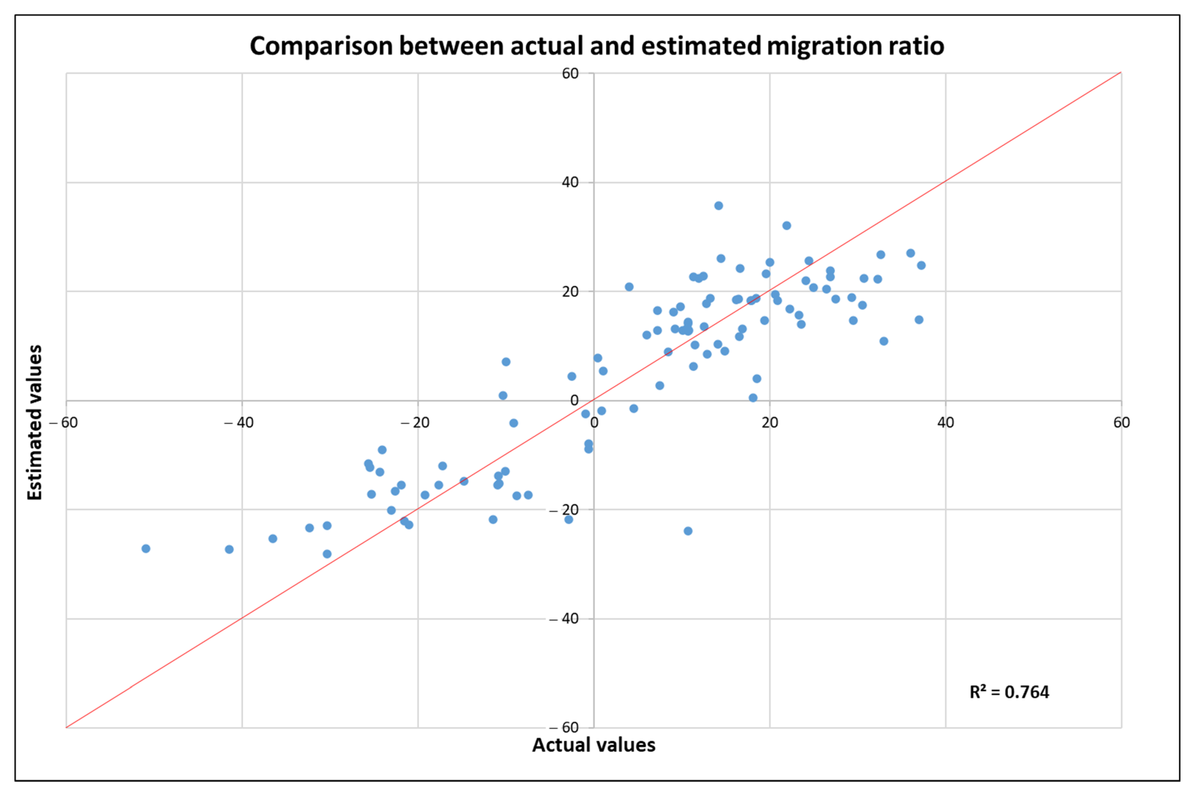
Figure 5 shows a scatter diagram in which the x-axis shows the actual values of the migration rate based on ISTAT data, and the y-axis shows the values calculated by applying the calibrated model. This graph confirms the goodness of the model since the points are included in a range not far from the bisector, the place of the points that would represent the perfect reproducibility of the phenomenon.

5. Discussion

The calibrated model allows us to estimate the impact of certain factors on the total migration balance between 2017 and 2022. After testing several models, combining different socio-economic and accessibility variables, we found a dependence of the migration rate on four variables: average income per capita, average property values in the area, overall accessibility by car (measured by travel time), and high-speed rail services.

The dependence on the average income per capita is in line with all the literature on international and national migratory phenomena. This variable was significant in many of the calibrated models, as well as the one with the highest correlation coefficient with the dependent variable, highlighting how the economic conditions of the place of destination are the main factor that induces a person to migrate from one area to another in the country. This factor is linked to the area’s employment conditions, so much so that the employment-related variables do not appear explicitly in the model, being somehow included in the average per capita income variable.

Property values also had a non-negligible influence on the phenomenon. Although the opposite effect could also be expected (higher property values and lower propensity to move due to the higher economic burden of renting or buying a house), areas with higher average real estate values are more attractive. This factor is also related to the general economic conditions in the area, but according to the results of significance tests, it also gives an independent contribution to the choice to migrate. It can, therefore, be assumed that the quality of the real estate fabric influences the studied phenomenon. This aspect of the problem would deserve a more in-depth study, in line with some research on the subject [49,50], but we will have to consider it in future research.

The variable of overall road accessibility, based on travel time, was another particularly relevant factor for interpreting the migration phenomenon. The possibility and ease of reaching where one decides to live and travelling from this to other places assumes significant relevance. After all, it is well known that the depopulation phenomena of certain areas are also significant due to their poor accessibility.

The fourth variable found to be significant in the model concerns high-speed rail services. In this case, as mentioned earlier, the negative coefficient of the variable seems to produce a counterintuitive result. An analysis of the findings in Table 4 shows that this variable was significant in some calibrated models (# 8, 9, 10, 11), always assuming a negative sign, which are also those with the highest values of the coefficient of determination. The interpretation is that a city better served by high-speed rail is also a city that can be reached more easily and more quickly and, therefore, allows those who have to work there to choose another place to establish their residence and be a commuter.

The results show how the accessibility of territories and the availability of transport services can influence internal migratory phenomena. Two of the four variables that emerged as significant refer to aspects linked to transport and accessibility. Most of the literature in this field, as reported in Section 2, studies migratory phenomena almost exclusively with regard to economic conditions and the labour market; this approach is largely justified for international migratory phenomena, in which the accessibility of a part of the territory, such as a province, is negligible compared to the other variables involved. When we move on to internal migration, economic and labour market factors certainly play the most important role, an aspect also confirmed by the calibrated model, but accessibility variables begin to assume greater importance. From the calibrated model, two contrasting trends were found. Road accessibility, which is a more general measure, had an attractive effect on internal migration: all other factors being equal, the most accessible areas were preferred to the less accessible ones. On the other hand, high-speed rail services had the opposite effect because they make it possible to live in a different area from the one where people work, as the fast connection makes it possible to organise a daily commute.

This result is in line with what was found in [41], where it was shown that cities well connected by high-speed railways attract skilled workers who prefer to travel rather than change their residence.

In Section 4, 25 models were summarised; of these, 12 were valid, that is, they satisfied the statistical tests and the tests on the sign of the coefficient. The model chosen, as mentioned previously, is the one that, among the valid models, had the highest R² value. This model relates the total migratory balance to four variables. Analysing all the calibrated models that are valid allowed us to identify which other variables were significant for the phenomenon, even if they could not be included in the best model because the statistical tests would not be respected. There were only two of these variables, which led to the calibration of a valid model but with a lower R² and, therefore, were less able to explain the phenomenon: rd_i and or_i. The first is overall accessibility based on distance within the road network; clearly, this could not be included in the calibrated model because it is closely correlated with rtt_i, which is the same measurement based on time but gave better results in the calibration of the model. The second variable is the employment rate; this is certainly important but closely correlated with the average per capita income, which performed better in the construction of the model. The other variables, on the other hand, were never significant in the models in which they were considered. The other socio-economic variables, probably because they are too specific, and the accessibility variables, probably because the variable considered, rtt_i, which represents overall accessibility, also partly includes accessibility to airports and accessibility weighted on the population.

The proposed study concerns Italy, and the calibrated model is valid only for this case study, which is based on specific input data. This study can contribute to the development of similar models for other European countries that present similar internal migration phenomena, which are present in many contexts where the socio-economic conditions are substantially different. The methodology proposed in this paper can be replicated in other contexts, as the data used are usually available and easily accessible in all developed countries. The construction of the road network graph, which is necessary to obtain most of the accessibility variables, must be implemented for specific case studies, and the procedure described can help in its construction. Another contribution that may help others replicate this study in other countries regards the variables that were tested in the model and some of the results obtained, such as, for example, the usefulness of considering the average value of the properties or the impact that the presence of a high-speed service has on the migration rate.

6. Conclusions

Like other European countries, Italy has a substantial disparity in socio-economic conditions between the different parts of its territory. In particular, a rich and industrialised north is contrasted by a poorer and less industrialised south. These strong differences, which have never been compensated for despite being known and indisputable since the post-war period, have generated internal migratory flows from the southern to the northern regions, as is clearly visible in the statistical data (see, for example, Figure 1 and Figure 3). This migration phenomenon has intensified in recent years; in particular, young people tend to emigrate for work reasons, as they do not find opportunities commensurate with their skills and education in their place of origin.

In this work, an attempt was made to model the phenomenon using multiple linear regression models, considering the influence that the accessibility of territories can have on their attractiveness. In addition to various accessibility variables, other socio-economic factors were considered, such as average income per capita, number of employees, level of employment, and so on. The specification and calibration of numerous models, which combined the different variables considered in various ways, led to the identification of a multiple linear regression model capable of representing the phenomenon with a good level of accuracy. The dependent variable was the total migration balance, while there were four independent variables, two socio-economic ones and two related to accessibility.

Road network accessibility, which can be calculated with a model of the Italian primary road network, was shown to have a positive effect on the migration phenomenon: the greater the accessibility of an area, the greater its attractiveness. The other accessibility variable, related to the availability of high-speed rail services, instead presented a negative effect; this can be interpreted as the variable being linked to ease of commuting and, therefore, avoiding moving to a city well served by fast rail transport.

The main contribution of this work to the literature is the study of how some accessibility parameters influence internal migration phenomena. The literature has almost always studied migration phenomena only in relation to socio-economic and labour market variables, which are certainly the most important, both for internal migration and, even more so, for international migration. The accessibility variables between small- and medium-sized territories, such as provinces, have not been considered previously, to the best of our knowledge.

Based on the results obtained, it is possible to make some recommendations for policymakers and transport planners. Firstly, overall accessibility is an essential factor in the development of a territory and also impacts migration. Making some areas of the country more accessible could mitigate some migratory trends, even if socio-economic aspects, which were also included in our model, are prevalent. Another important indication is that, to avoid a high concentration of population in some cities and the depopulation of other areas of the country, it is necessary to improve high-speed rail services, which allow commuting for work or study, limiting the depopulation of more economically and socially depressed areas.

Future research can be directed in different directions. Firstly, non-linear models or experiments on other European countries with similar migratory phenomena could be proposed; secondly, similar models could be proposed to verify how accessibility can influence international migration; and, finally, more complex models could be studied and applied, such as spatial econometric models, temporal dynamic models, a longitudinal panel data approach, or machine learning techniques, which can interpret even more complex variables that could influence migratory phenomena.