Article

Comparative Analysis of Japanese Rice Wine Export Trends: Large Firms in the Nada Region vs. SMEs in Other Regions

1
Centre for Finance, Technology and Economics at Keio, Keio University, Tokyo 108-8345, Japan
2
Center for Advanced Intelligence Project, RIKEN, Tokyo 103-0027, Japan
3
Faculty of Economics, Keio University, Tokyo 108-8345, Japan
*
Author to whom correspondence should be addressed.
World 2024, 5(3), 700-722; https://doi.org/10.3390/world5030036
Submission received: 19 June 2024 / Revised: 19 August 2024 / Accepted: 22 August 2024 / Published: 27 August 2024

Abstract

:
In recent decades, Japanese rice wine, sake, exports to international countries have developed tremendously. Recently, in particular, sake exports are increasing in both volume and unit value due to factors such as the registration of Japanese cuisine as an intangible cultural heritage of UNESCO in 2013 and the economic situations including the rapid depreciation of Japanese yen. However, there are no studies which investigated sake exports via empirical methods as far as we know. In this study, we constructed hierarchical Bayesian models and analyzed unbalanced panel datasets on the export of Japanese sake to China, Hong Kong SAR China, Singapore, Taiwan and the US by using a Markov chain Monte Carlo (MCMC) method and an ancillary-sufficiency interweaving strategy (ASIS) as the first empirical study of Japanese sake export. As a result, it was found that the trends in export volume and unit value to China, Hong Kong SAR China, Singapore and the US were significantly positive. In addition, although Taiwan had a negative trend before UNESCO registration, the trend became positive after its registration. Based on these results, it can be concluded that Japanese sake has been booming worldwide, though the degree may vary from country to country. Especially, we found that the UNESCO registration of Japanese food, Washoku, has significant effects on booming sake exports both in terms of volume and unit value. Finally, we divided the sake export data by regional customs offices in charge and conducted a detailed analysis on regional heterogeneity in sake exports. From the results, we found there were some different trends among regions.

1. Introduction

Various alcoholic beverages are available worldwide, many based on different countries’ unique cultures and customs. For example, Japan is known for its sake, a type of rice wine. This alcoholic beverage has been brewed from ancient times, at least from the seventh century (According to the Japanese Sake and Shochu Makers Association, the description that Japanese people were brewing sake in the seventh century was found in an old Japanese historical record called Harima no kuni fudoki). In current days, most Japanese people have either consumed sake or know the name of sake even if they have never consumed it. Sake is not only drunken on a daily basis, but is also frequently used for ceremonial occasions. For instance, sake is used for wedding and funeral gifts, gifts for close friends and business partners, and so on. Thus, sake is very familiar with Japanese culture. With the globalization of the modern age, sake has gained recognition around the world. Sake is often served in an auspicious wooden sake cup called “masu”, and is associated with Japanese culture such as Shinto and Buddhist rituals (Figure 1).
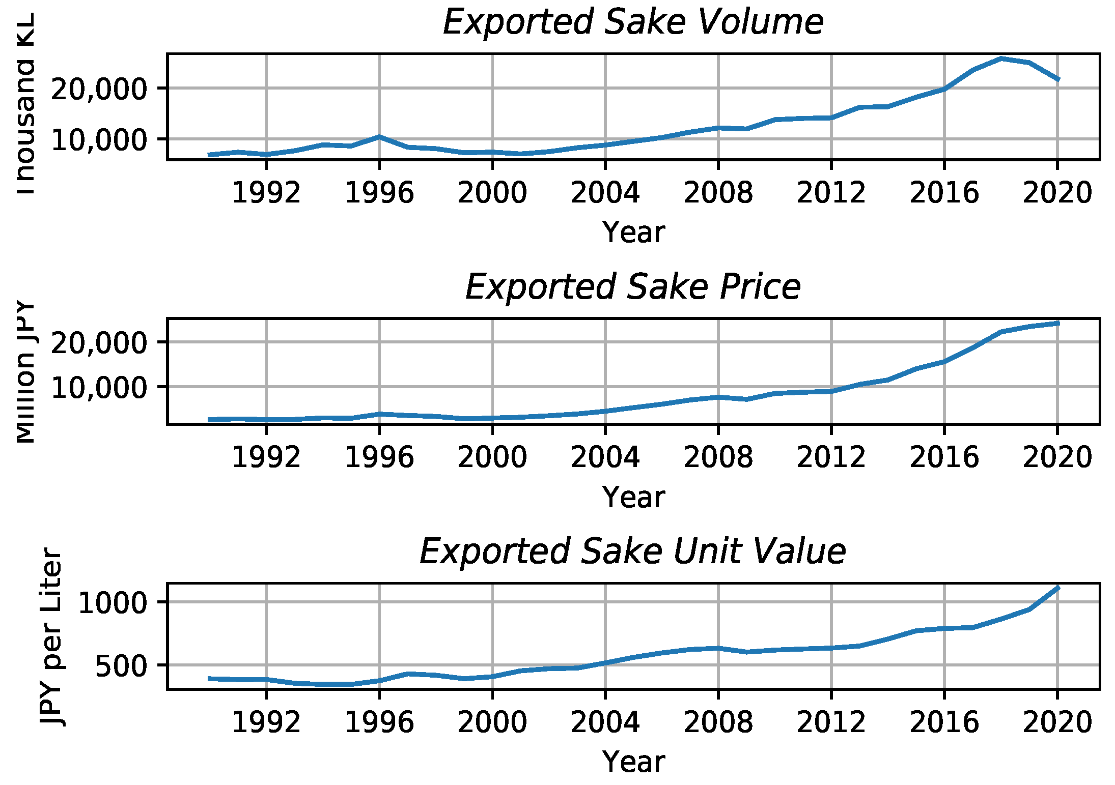
Sake exports have drastically increased over the last three decades (Figure 2). Notably, the growth in the export volume was faster than the export value. To confirm this fact, the growth rate of the unit export price has been much more rapid than the growth rate of the export volume, indicating that sake is becoming increasingly expensive in the overseas market. According to the Japanese National Tax Administration Agency [1], the average export unit price was JPY 1323, almost double the average domestic price of JPY 736.
One possible factor contributing to this development is the inclusion of Japanese cuisine on UNESCO’s Intangible Cultural Heritage List in 2013. People outside Japan have become aware of traditional Japanese cuisine, washoku, especially since it was included in the 2013 Intangible Cultural Heritage List of the United Nations Educational, Scientific and Cultural Organization (UNESCO). Shinato and Kato [2] argue that the Japanese government began promoting sake after the UNESCO registration. Kishi [3] notes that the number of restaurants serving Japanese food worldwide doubled after the UNESCO registration. According to the Japan External Trade Organization (JETRO) [4], in the past, only a few restaurants in China served Japanese cuisine; however, since the UNESCO registration and the economic boom due to the Beijing Olympics in 2008, the number of Japanese restaurants reached 900 in Shanghai and 500 in Beijing. Moreover, according to JETRO [5], the consumption of cheap sake in Taiwan, formerly from major affiliated companies, has risen since 2015 as more department stores and specialty shops offer high-end sake. The UNESCO registration might also significantly impact the North American market, where Japanese cuisine rapidly spread in the 2010s. Fujishiro [6] argues that the number of restaurants providing washoku tripled after the UNESCO registration.
Another factor in export growth is the widening price gap between the domestic and overseas markets. Japan suffered from stagnation and deflation for the last three decades, while other countries experienced inflation during the same period. Furthermore, the depreciation of the JPY since the beginning of the Quantitative and Qualitative Easing (QQE) policy by the Bank of Japan in 2013 also contributed to this trend. As a result, the price gap in alcoholic beverages between Japan and other countries has been widening, which helps the sale of sake in overseas markets.
In any case, the future is not a simple continuation of the past. Therefore, it is essential to understand what factors determine the trend of sake export (shown in Figure 2) so that Japanese sake breweries can sustain the current upward trend of sake export. To our knowledge, no previous studies have examined sake export. Our study conducts a panel data regression analysis of sake exports to Japan’s major trade partners and investigates the influences of socio-economic variables upon sake exports.
Although we could not find any previous studies on sake exports, there are several studies on the export of other alcohol beverages in the literature. For example, Bouët et al. [7] showed that income elasticity of demand had a significant impact on Cognac export. Furthermore, Bargain [8] found that the income and price effects of French wine export to China differed according to the wine-growing regions in France. Cardebat and Figuet [9] argued that the appreciation of the Euro increased the share of premium wines in French wine exports. Candau [10] found that there were some differences in wine export by transportation. Capitello [11] showed price elasticities differed by kinds of imported wine in the Chinese market. Fontagné [12] implied that unit value had significant impact on the determinants of high-quality wines in European Market. Following the above studies on alcoholic beverages, we adopt a log–log model specification for the key variables in the panel data regression model. The number of countries in the panel data is relatively small (we have only five countries, as described in Section 2); therefore, we apply hierarchical Bayesian modeling to the panel data regression model and estimate it with an efficient Markov chain Monte Carlo (MCMC) method called an ancillary-sufficiency interweaving strategy (ASIS) to improve the sampling efficiency of MCMC. In the next section, we will describe the data used in the analysis and elaborate on the estimation procedure. In sum, our modeling and estimation will be performed in the following process:
  • Construct a log-log model in the regression model
  • Estimate the model with the UNESCO registration and the other facts via hierarchical Bayesian modeling.
This paper is organized as follows. Section 2 presents the datasets for our empirical research and explains the estimation procedure. Section 3 shows the estimation results of panel data regression models for volume and unit value sake exports; we also discuss their implications and how socio-economic variables influence sake exports. However, it can be argued that these analyses are insufficient when the industrial structure of the sake industry is taken into account because the industrial structure of the sake industry differs significantly between certain region and others. The main region is called Nada. The Nada region is good for obtaining water suitable for sake brewing, and its location near the port is advantageous for the distribution of sake. So from the 18th century, Nada has been the center of sake brewing. As a result, in the Nada region, an agglomeration of breweries occurred and large companies were set up to produce large volumes of sake. In contrast, the other areas still have breweries which belong to small and medium enterprises. So in Section 4, we explore possible export structure heterogeneity between Nada, Japan’s central sake brewing region, and the rest of the country. Finally, Section 5 summarizes our research findings and draws a conclusion.

2. Datasets and Estimation Procedure

2.1. Datasets

The dataset for this study consists of volume and unit value of sake exports, consumer price indexes and nominal exchange rates. The export data were obtained from the Trade Statistics of Japan Ministry of Finance, and the rest of the data were obtained from the Nikkei Economic Electronic Databank System, a data providing service operated by Nikkei Inc. Due to data availability, we set the sample period from 1995 to 2021 for our empirical analysis of sake export. We selected five major countries that import the most: China, Hong Kong SAR China, Singapore, Taiwan China, and the United States (US). These five countries have been continuously importing sake from Japan during the sample period, and the export of sake to them accounts for around 60% of the total volume of sake exported during the sample period.
Our analysis considers a panel data regression model for the five countries. The dependent variable is each country’s export volume or export unit value (export value divided by export volume). Common independent variables for all countries include (a) export unit value (Unit), (b) consumer price index (CPI), (c) nominal exchange rate (NER), and (d) monthly seasonal dummy variables excluding January. The first three variables are based on Bargain [8] Bouët et al. [7], Mitchell [13], and Nelson [14] and we examine how they influence each country’s sake export. We use Nikkei Currency Indices instead of nominal exchange rates to control mutual influences among different currencies. We use log-log specification for panel data regression models; the dependent variables, Unit, CPI and NER are in the natural logarithm. For a regression model of the export unit value, Unit will be dropped since it is used as the dependent variable. Table 1 shows the descriptive statistics of these variables. Note that the panel data is unbalanced. From the statistics, we can argue some facts for the sake export. For instance, it can be identified that the average unit value is significantly lower in Taiwan than in the other four countries while it is the second largest export quantity after the US. As we stated in the introduction, Taiwan imported mainly cheap sake until the 2010s, so this data reflects the fact. Next, the US has the largest sake market in terms of quantity and has a high unit value. Finally, Singapore has a minimum quantity but has a higher unit value. This means that only luxury sake is exported to Singapore. Sake brewing is inherently seasonal, and the process is susceptible to temperature and exhibits seasonal fluctuations. Similarly, the rice harvest is also seasonal. To capture possible seasonal fluctuations in sake exports, we add monthly seasonal dummy variables to the panel data regression model; we exclude the dummy variable for January to avoid multicollinearity.
In addition to the common independent variables, we introduce country-specific constant terms and time trends to the panel data regression model. To capture heterogeneity among countries, the constant term and the slope of the time trend can differ among the countries. In the literature, several studies found supportive evidence for such heterogeneity. For example, Fogarty [15] and Nelson [14] found that countries in the European Union had different trends in the elasticity values of alcoholic beverages. Lombardi et al. [16] also showed that the trends of bottled wine shipments within the EU varied by country. Bargain [17] applied a time trend to export models of alcoholic beverages. Mitchell [13] found that time-dependent taste changes significantly determined wine and beer demand in the EU. Connolly et al. [18] showed that short-time trends significantly impacted beer sales in Connecticut, US, after the beer sales were admitted even on Sunday. Hart and Altson [19] found that historical alcohol consumption trends in the US differed from geographical factors, like regions or states.
Furthermore, to analyze the effect of the UNESCO registration of Japanese cuisine, we add the UNESCO dummy variable and the UNESCO time trend to the model. The UNESCO dummy variable takes 1 after the registration and takes 0 before while the UNESCO time trend starts from 2013-03 and ends in 2021-12. We also allow the coefficient of these variables to be different among countries to capture the heterogeneity in sake exports.
Table 2 summarizes two model specifications we consider for the panel data regression model. Model I is the base model to examine the impacts of the key variables on sake exports. Model II is for checking the influence of the UNESCO registration of Japanese cuisine.

2.2. Estimation Procedure

These models are expressed as the following panel data regression model
y i t = w t γ i + x i t β + ϵ i t , ϵ i t i . i . d . N ( 0 , σ ϵ 2 ) , i { 1 , , N } , t { 1 , , T i } ,
where
  • y i t — export volume or unit value of sake to the i t h country in the t t h period;
  • w t — a vector of the constant term and the time trend in the t t h period;
  • x i t — a vector of the common independent variables of the i t h country in the t t h period.
In Equation (1), Japanese sake breweries export their sake to N countries and we have T i periods of data on sake exports to the i t h country. In out study, N = 5 (China, Hong Kong, Singapore, Taiwan and the United States) and T i of each country is shown in Table 1. γ i in Equation (1) includes the intercept (constant term) and slope of the country-specific time trend of the i t h country to capture the heterogeneity among countries. In case of Model II, it also include the intercept and slope corresponding a possible regime shift before and after the UNESCO registration of Japanese cuisine in 2013. β in Equation (1) includes the regression coefficients for the common independent variables including monthly seasonal dummy variables.
Then, defining vectors and matrices as
y i = y i 1 y i T i , W i = w 1 w T i , X i = x i 1 x i T i , ϵ i = ϵ i 1 ϵ i T i ,
the regression model of Equation (1) corresponding to the sake export to the i t h country can be summarized as
y i = W i γ i + X i β + ϵ i , ϵ i N ( 0 T i , σ ϵ 2 I T i ) ,
where 1 T i is a T i × 1 -vector whose elements are all ones, 0 T i is a T i × 1 -vector whose elements are all zeros, and I T i is the T i -dimensional identity matrix. Finally, stacking up vectors and matrices as
y = y 1 y N , W = W 1 W N , X = X 1 X N , Z = W X , ϵ = ϵ 1 ϵ N , γ = γ 1 γ N , δ = γ β ,
the regression model for all N countries is summarized as
y = W γ + X β + ϵ = Z δ + ϵ , ϵ N 0 T , σ ϵ 2 I T , T = i = 1 N T i .

2.3. Bayesian Estimation

Next, we set up the posterior distribution to conduct a hierarchical Bayesian analysis on the regression model in Equation (1). Since the conditional distribution of y under a given Z in Equation (3) is N ( Z δ , σ ϵ 2 I ) , the likelihood of the unknown parameter ( δ , σ ϵ ) is
p ( y | Z , δ , σ ϵ ) ( σ ϵ 2 ) T 2 exp 1 2 σ ϵ 2 ( y Z δ ) ( y Z δ )
( σ ϵ 2 ) T 2 exp i = 1 T i e i t 2 2 σ ϵ 2 , e i t = y i t w t γ i x i t β .
We assume the following prior distribution for the parameter ( δ , σ ϵ ) .
δ N μ , Σ , μ = 1 N μ γ μ β , Σ = I N Σ γ Σ β ,
σ ϵ C + ( 0 , s ϵ ) ,
where ⊗ is the Kronecker product, Σ γ is supposed to be diagonal, and C + ( · ) is a half-Cauchy distribution,
p ( σ ϵ | s ϵ ) = 2 s ϵ π ( σ ϵ 2 + s ϵ 2 ) , σ ϵ > 0 , s ϵ > 0 .
We assume the half-Cauchy distribution as Gelman [20] and Gelman [21] recommended for hierarchical models.
Note that the prior distribution in Equation (6) is equivalent to assuming
γ i j i . i . d . N ( μ γ j , σ γ j 2 ) , i { 1 , , N } , j { 1 , , K } , β N ( μ β , Σ β ) ,
where γ i j and μ γ j are the j t h element of γ i and μ γ , respectively, σ γ j 2 is the j t h diagonal element of Σ γ , and K is the number of elements in γ . K = 2 in Model I and K = 4 in Model II.
In the prior distribution of the parameter ( δ , σ ϵ ) , ( μ β , Σ β ) in Equation (6) and s ϵ in Equation (7) are fixed to a specific value as hyperparameters. In the prior distribution of { μ γ j , σ γ j } j = 1 K in Equation (8), however, we set the following hierarchical prior distribution:
μ γ j N ( φ γ , τ γ 2 ) , σ γ j C + ( 0 , s γ ) , j { 1 , , K } ,
and attempt to estimate it simultaneously with ( δ , σ ϵ ) using a Bayesian approach.
With the use of hierarchical Bayesian analysis, the values of { μ γ j , σ γ j } j = 1 K in the prior distribution (8) are not fixed as hyperparameters, but can be estimated simultaneously with other parameters to construct a flexible prior distribution. Another advantage of hierarchical Bayesian analysis is that the shrinkage method can be used to stabilize the estimation of individual effects. Additionally, ( φ γ , τ γ 2 , s γ ) in Equation (9) are fixed to specific values as hyperparameters. In this study, we set the values of the hyperparameters ( μ β , Σ β , φ γ , τ γ 2 , s γ , s ϵ ) as
μ β = 0 14 , Σ β = 100 I 14 , φ γ = 0 , τ γ 2 = 100 , s γ = s ϵ = 1 .
Note that the dimension of β is 14, which is equal to the number of the common independent variable (3) plus the number of monthly seasonal dummy variables (11).
In summary, we can conclude that the parameters to be estimated in the hierarchical Bayesian analysis of the regression model (1) for sake export are
θ = δ , μ γ , diag ( Σ γ ) , σ ϵ = ( γ 1 , , γ N , β , μ γ 1 , , μ γ K , σ γ 1 , , σ γ K , σ ϵ ) ,
and the posterior distribution of unknown parameters θ is derived as
p ( θ | D ) p ( y | Z , δ , σ ϵ ) p ( θ ) , D = ( y , Z ) ,
where p ( y | Z , δ , σ ϵ ) is the likelihood in Equation (4) and p ( θ ) is the product of the prior distributions in Equations (6), (7) and (9). Unfortunately, the posterior distribution (11) cannot be evaluated analytically. Therefore, we will proceed with the hierarchical Bayesian analysis by using the Markov chain Monte Carlo (MCMC) method. The conditional posterior distribution of each parameter is derived as follows (see Appendix A).
δ | D , θ δ N σ ϵ 2 Z Z + Σ 1 1 σ ϵ 2 Z y + Σ 1 μ , σ ϵ 2 Z Z + Σ 1 1 ,
μ γ j | D , θ μ γ j N σ γ i 2 i = 1 N γ i j + τ γ 2 φ γ σ γ j 2 N + τ γ j 2 , 1 σ γ j 2 N + τ γ 2 ,
σ γ j 2 | D , θ σ γ j , ξ γ j IG N + 1 2 , i = 1 N ( γ i j μ γ j ) 2 2 + 1 ξ γ j , ξ γ j | σ γ j IG 1 , 1 σ γ j 2 + 1 s γ 2 ,
σ ϵ 2 | D , θ σ ϵ , ξ ϵ IG T + 1 2 , i = 1 N t = 1 T i e i t 2 2 + 1 ξ ϵ , ξ ϵ | σ ϵ IG 1 , 1 σ ϵ 2 + 1 s ϵ 2 ,
where θ a indicates that the parameter a is excluded from θ , and IG ( a , b ) is the inverse gamma distribution
p ( x | a , b ) = b a Γ ( a ) x ( a + 1 ) e b x .
In the conditional posterior distribution of Equations (14) and (15), new latent variables ( ξ γ 1 , , ξ γ K , ξ ϵ ) are introduced. This is because x C + ( 0 , a ) is expressed as
x 2 | z IG 1 2 , 1 z , z IG 1 2 , 1 a 2 ,
and is used to derive Equations (14) and (15) (see Appendix A for details).
The conditional posterior distributions in Equations (12)–(15) have all known efficient random number generation algorithms, such as the normal and inverse gamma distributions. Therefore Gibbs sampling can be used to generate parameters θ from their posterior distribution. It turns out that a simple Gibbs sampling algorithm consisting of the conditional posterior distribution of Equations (12)–(15) is inefficient in drawing Monte Carlo samples from the posterior distribution when it was applied to the exported sake data used in this study. To overcome this inefficiency, we apply the ASIS proposed by Yu and Meng [22] to { γ i } i = 1 N . To demonstrate the ASIS algorithm used in this study, we first assume that ( γ 1 , , γ N , μ γ 1 , , μ γ K ) are generated by Gibbs sampling, and consider the following transformation.
γ ˜ i = γ i μ γ , y ˜ i t = y i t w t γ ˜ i , i { 1 , , N } , t { 1 , , T i } .
Then Equation (1) is rewritten as
y ˜ i t = w t μ γ + x i t β + ϵ i t , ϵ i t i . i . d . N ( 0 , σ ϵ 2 ) .
Thus, Equation (18) becomes
y ˜ = Z ˜ δ ˜ + ϵ , ϵ N ( 0 T , σ ϵ 2 I N ) , y ˜ = y ˜ 11 y ˜ N T N , Z ˜ = w 11 x 11 w N T N x N T N , δ ˜ = μ γ β ,
Then the conditional posterior distribution of δ ˜ is obtained as
δ ˜ | D , θ δ N σ ϵ 2 Z ˜ Z ˜ + Σ ˜ 1 1 σ ϵ 2 Z ˜ y ˜ + Σ ˜ 1 μ ˜ , σ ϵ 2 Z ˜ Z ˜ + Σ ˜ 1 1 , μ ˜ = φ γ 1 N μ β , Σ ˜ = τ γ 2 I N Σ β ,
by exactly the same procedure with Equation (12); thus, the Gibbs sampling with the addition of ASIS can be summarized as follows (In short, the prior distribution of δ ˜ is N ( μ ˜ , Σ ˜ ) ).
Step 1
Given the sth generated θ ( s ) , apply Gibbs sampling based on Equations (12)–(15) to generate θ ( s + 0.5 ) and compute
γ ˜ i ( s + 0.5 ) = γ i ( s + 0.5 ) μ γ ( s + 0.5 ) .
Step 2
Given θ ( s + 0.5 ) , apply Gibbs sampling based on Equations (20) and (14)–(15) to generate ( β ( s + 1 ) , μ γ 1 ( s + 1 ) , , μ γ K ( s + 1 ) , σ γ 1 ( s + 1 ) , , σ γ K ( s + 1 ) , σ ϵ ( s + 1 ) ) , and compute
γ i ( s + 1 ) = γ ˜ i ( s + 0.5 ) + μ γ ( s + 1 ) .
In this study, we use this Gibbs sampling to generate a Monte Carlo sample { θ ( s ) } s = 1 S of θ from the posterior distribution, and conduct the hierarchical Bayesian analysis of sake export.

3. Hypotheses and Estimation Results

We consider the following hypotheses following the previous studies.
Hypothesis 1 (H1).
The trend of sake export may exhibit heterogeneity among countries as demonstrated for other alcoholic beverages.
Hypothesis 2 (H2).
Unit , CPI and NER may significantly impact sake exports. According to previous studies (Bargain [8] and Bouët [7]), Unit may negatively affect sake exports.
Hypothesis 3 (H3).
Seasonal effects may exist.
H1 and H2 seem legitimate in light of the previous studies but we may need to elaborate on H3. Traditional sake brewing methods require sensitive temperature control (See more details on Saito and Nakatsuma [23]). Without any modern temperature management equipment, it is impossible to brew sake for all seasons, especially during a hot summer. For this reason, most sake breweries start brewing in late autumn. This timing is also related to the harvest time of rice, the key material for sake, which is harvested in autumn, too. Moreover, unlike wine, sake is a fermented alcoholic beverage. So the longer it is brewed, the more its quality deteriorates, albeit gradually. This nature of sake puts pressure on breweries to sell off sake brewed during the winter by the next summer. Thus, we expect seasonal fluctuations in sake exports due to supply-side constraints of sake brewing.

3.1. Estimation Results of Export Volumes

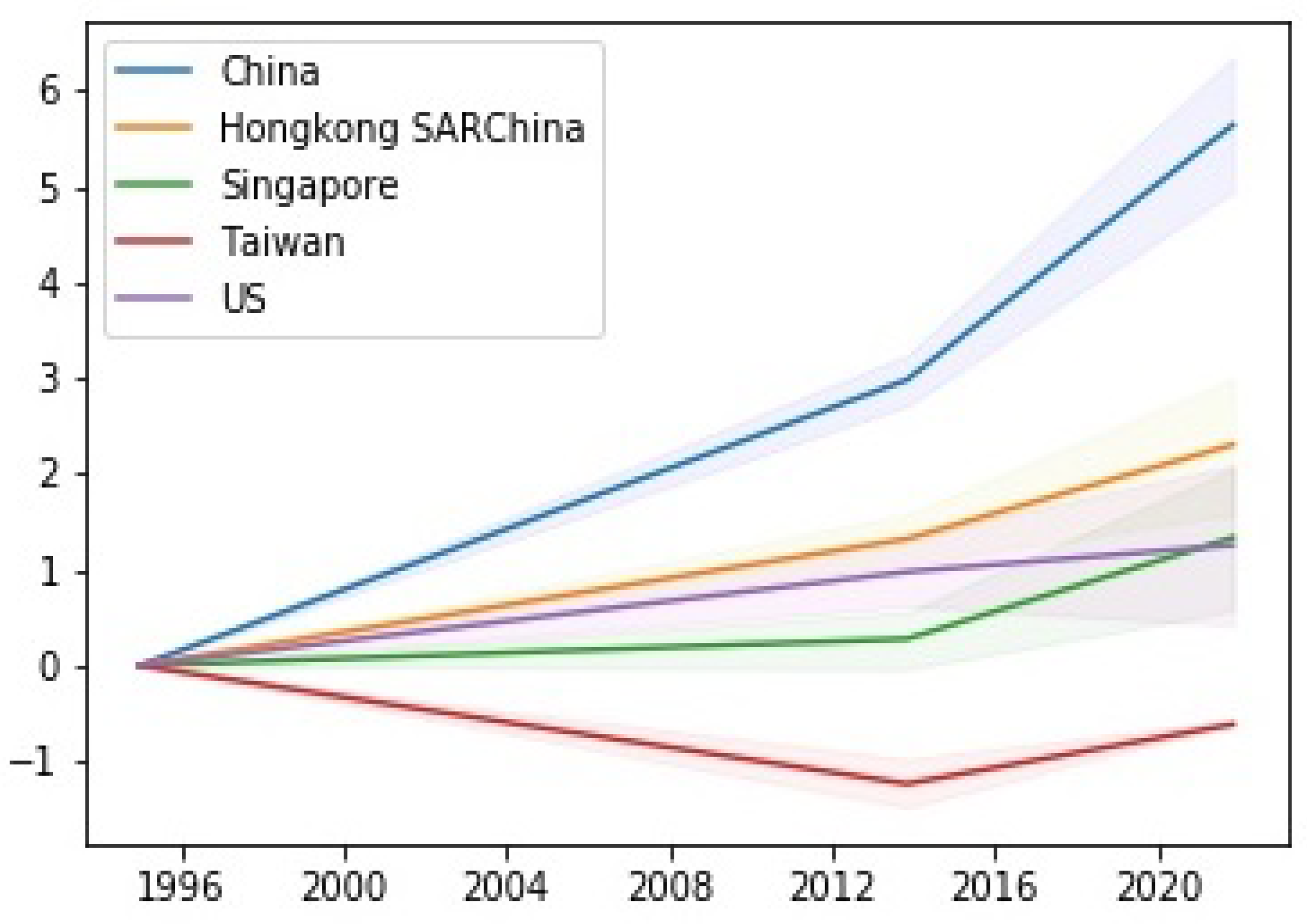
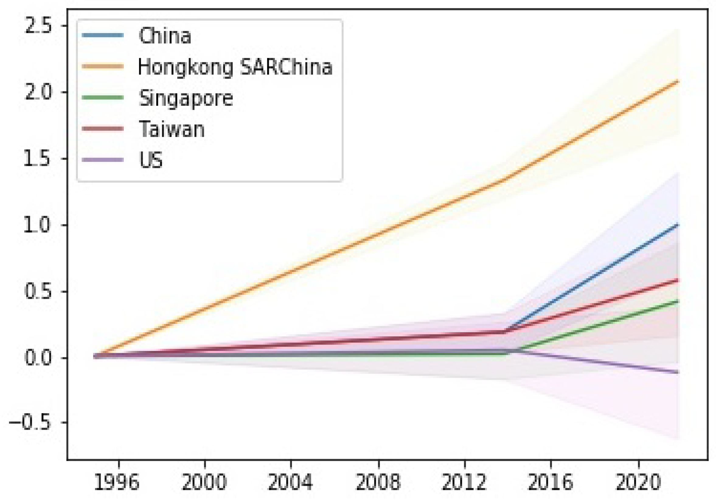
Table 3 shows the estimation results of the panel data regression model in Equation (1). In Table 3, Intercept (I) and Intercept (II) represent the country-specific intercepts (constant terms) in the panel data regression model, respectively. Slope (I) and Slope (II) represent the country-specific slope of the time trend, respectively. Then we illustrated Slope (II) in Figure 3. Finally, Intercept (II, UNESCO) and Slope (II, UNESCO) represent the country-specific coefficient of the UNESCO registration dummy variable and the UNESCO registration time trend, respectively (In this section, “Hong Kong” is the abbreviation of “Hong Kong SAR China” in tables and sentences).
In Table 3 and Figure 3, the number without parentheses is the mean of the posterior distribution of each coefficient; the number within parentheses is the standard deviation of the corresponding posterior distribution. The double asterisk indicates that the 95% interval of the posterior distribution of the corresponding coefficient does not include zero. Following the convention, we conclude that the coefficient is “significant” if its 95% interval does not include zero. We follow the same rules for all tables and figures below. The notation implies the coefficient is “significant” in 95% levels in the all following tables.
In Table 3, Intercept (I) is significant for Hong Kong and Taiwan, while Intercept (II) is insignificant for any country. Intercept (II, UNESCO) is significantly negative for Hong Kong.
The export volume on the left-hand side of Equation (1) is in the natural logarithm; therefore, the slope of the trend can be interpreted as the growth rate of sake export to the corresponding country. In Table 3, Slope (I) is significant for all five countries; it is significantly positive except for Taiwan, and it is highest for China. This result may reflect a steady growth of sake exports to China during the sample period. Slope (II) shows a similar pattern, though it is insignificant for Singapore.
Note that Slope (II) is the growth rate of sake export before the UNESCO registration of Japanese cuisine in 2013 while the sum of Slope (II) and Slope (II, UNESCO) is the growth rate after the UNESCO registration. Thus, Slope (II, UNESCO) indicates a change in the growth rate of sake exports after the UNESCO registration. It is graphically illustrated in Figure 3. It is significantly positive for four countries except for the US. This result indicates that the UNESCO registration might accelerate the growth of sake exports to these four countries. Unsurprisingly, the UNESCO registration boosted sake exports to countries like China and Hong Kong where sake exports were already thriving. As we mentioned in Section 1, the rapid increase in Japanese restaurants in China after the UNESCO registration had a significant impact on the increase in sake export volume in the Chinese market. For Singapore and Taiwan, the impacts were more dramatic. Before the UNESCO registration, the growth rate of sake export to Singapore was virtually zero and it was negative for Taiwan. From the estimation results in Table 3, the growth trend of sake exports to Singapore increased after the UNESCO registration. At the same time, the downward trend of the growth rate of export to Taiwan was clearly changed positive. This result is also consistent with the cases we have described in Section 1. It is considered that after the UNESCO registration, more premium sake has been exported to Taiwan. Conversely, the insignificant Slope (II, UNESCO) for the US may need some explanation. We conjecture that Japanese cuisine was already popular in the US before the UNESCO registration; therefore, it could not contribute so much to accelerating the growth of sake exports. Overall, the results in Table 4 show significant heterogeneity in sake exports among the countries, which supports H1.

3.2. Estimation Results of Export Unit Values

Next, we examine the impacts of economic variables upon sake exports with the estimation results in Table 4. For both Model I and Model II, Unit and CPI are significant and their signs are consistent with the conventional wisdom in economics. As for NER, it is insignificant in Model II; thus, we can support H2 completely in Model I, but only partially in Model II. Arguably, the trend shift due to the UNESCO registration confounded the effect of exchange rate fluctuations because the UNESCO registration and the QQE, which caused a sharp depreciation of the JPY, occurred in the same year.
The posterior statistics in Table 5 indicate the monthly seasonal effects in sake exports. Note that the base month is January. For both Models I and Model II, exports are significantly positive from October to April. The numbers from October to December may be related to the fact that sake breweries start brewing in October, which means they start exporting freshly brewed sake during this period. The period from February to April may be related to sake contests. Many sake breweries regularly participate in contests regarding the quality of premium sake. If they are successful, it will be an excellent boon for marketing; hence, winning the contest is their top priority. However, brewing premium sake is labor-intensive and hinders daily brewing operations. Since breweries start preparing for the contest in January, their daily operation will slow down. Only after they finish brewing premium sake for the contest can breweries start exporting new sake again. As a result, we observe seasonal fluctuations shown in Table 5.
In addition to the volume of sake export, we estimated panel data regression models of the unit value of sake export. Using the unit value of sake export as the dependent variable in Models I and II, we computed the posterior statistics of the parameters in Equation (1). They are shown in Table 6 and Table 7.
In Table 6, Intercept (I) and Intercept (II) are significantly negative for all countries. As for Intercept (II, UNESCO), it is significant for Hong Kong (significantly negative) and Taiwan (significantly positive).
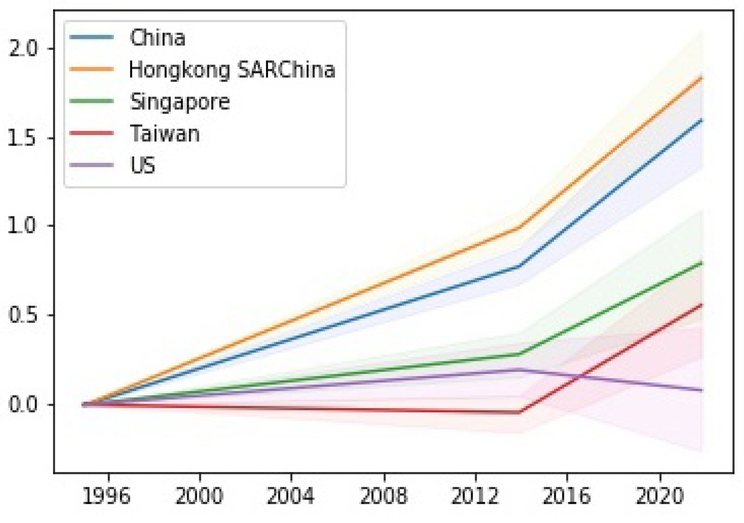
As shown, China and Hong Kong move in a similar direction. Slope (I), Slope (II) and Slope (II, UNESCO) in Table 6 are all significantly positive for China and Hong Kong. This result indicates that the unit value of imported sake has been rising for these countries, which is consistent with the rapid growth of the Chinese economy during the sample period. The economic growth made the people wealthier and higher-grade sake became more affordable for them. Notably, the rise in the unit value was accelerated by the UNESCO registration for these countries as is shown in Figure 4.
We may put Singapore and Taiwan into another category. In Table 6, Slope (I) for Singapore and Taiwan is significantly positive, as is China and Hong Kong; thus, the same factor, economic growth, played the same role in making more expensive sake affordable. Conversely, if we look into Slope (II) and Slope (II, UNESCO), we obtain a slightly different perspective on the unit value of imported sake in these countries. Before the UNESCO registration, Slope (II) was insignificant for Singapore and it is even significantly negative for Taiwan; therefore, we may conclude that they preferred less expensive sake during that period. After the UNESCO registration, on the other hand, Slope (II, UNESCO) was significantly positive for both Singapore and Taiwan and the absolute value of the coefficient was comparable to that of China and Hong Kong. This trend may imply that the people in Singapore and Taiwan started to accept higher-grade sake after the UNESCO registration.
Consumer preference in the US seems different from that of Asian countries. Slope (I) is insignificant and the posterior mean is virtually zero for the US, meaning that the unit value of imported sake remains unchanged in the sample period. Furthermore, Slope (II) is significantly positive but Slope (II, UNESCO) is significantly negative, which implies that the upward trend in the unit value was reversed after the UNESCO registration. This seemingly confusing result may be explained by the fact that, in the US, the UNESCO registration increased the number of Japanese restaurants. This increase led to a surge in the volume of sake exports, possibly resulting in a decline in the unit value.
In Table 7, both CPI and NER are significantly positive in Model I, but NER is not significant in Model II. This result is the same as the volume regression in Table 4.
In Table 8, the unit value is higher after June. This is probably due to the fact that sake breweries are unable to ship more expensive sake until June when contests on premium sake finish and breweries can start exporting.
From these analyses, we can argue three facts. Firstly, China and Hong Kong were originally on a growth trend in terms of both volumes and unit values, but the UNESCO registration has further accelerated their growth. Secondly, it can be said that Singapore originally had a near-constant growth rate, but the UNESCO registration accelerated the growth of the sake export at a rapid increase, both with regard to volume and unit value. And it was also confirmed that although Taiwan’s growth rate had been on a downward trend in terms of both volume and unit value, the growth rate has turned to an upward trend since the UNESCO registration. So the registration had great impact on export growth in Taiwan. Finally, the UNESCO registration did not have significant effects on sake exports to the US. So we confirmed some heterogeneity in the growth rates of sake exports.

4. Extension: Differences between Traditional Sake Brewing Region Nada and the Others

So far we have used export data on the overall sake brewing industry. The sake brewing industry’s structure differs significantly in Nada compared to the rest of Japan. The Nada region has played a significant role in the Japanese sake brewing industry. Akiyama [24] stated that, in the Edo period (1603–1868), Nada was a region blessed with good quality rice and water suitable for sake brewing, as well as good maritime transportation. This led to an industrial agglomeration of sake breweries in the Nada region which has had a significant impact on the sake brewing industry even today. The Japanese National Tax Agency reports that almost half of the sake consumed in the domestic market is brewed by breweries in the Nada region. So it is safe to say that large-scale sake breweries, which are called major sake companies, are almost exclusively concentrated in this region.
To examine any differences between sake breweries in the Nada region and the rest of Japan, we first estimated panel data regression models of the volume of sake export from the Nada region (We substituted y i t in Equation (1) for the export volume or unit value of Nada and Unit for the unit value of Nada). Data on sake exported from Kobe Customs is used as a proxy variable for sake exported from the Nada region because sake from Nada is mostly exported from Kobe (represented by Kobe Customs reports).

4.1. Estimation Results of Export Volumes in Nada

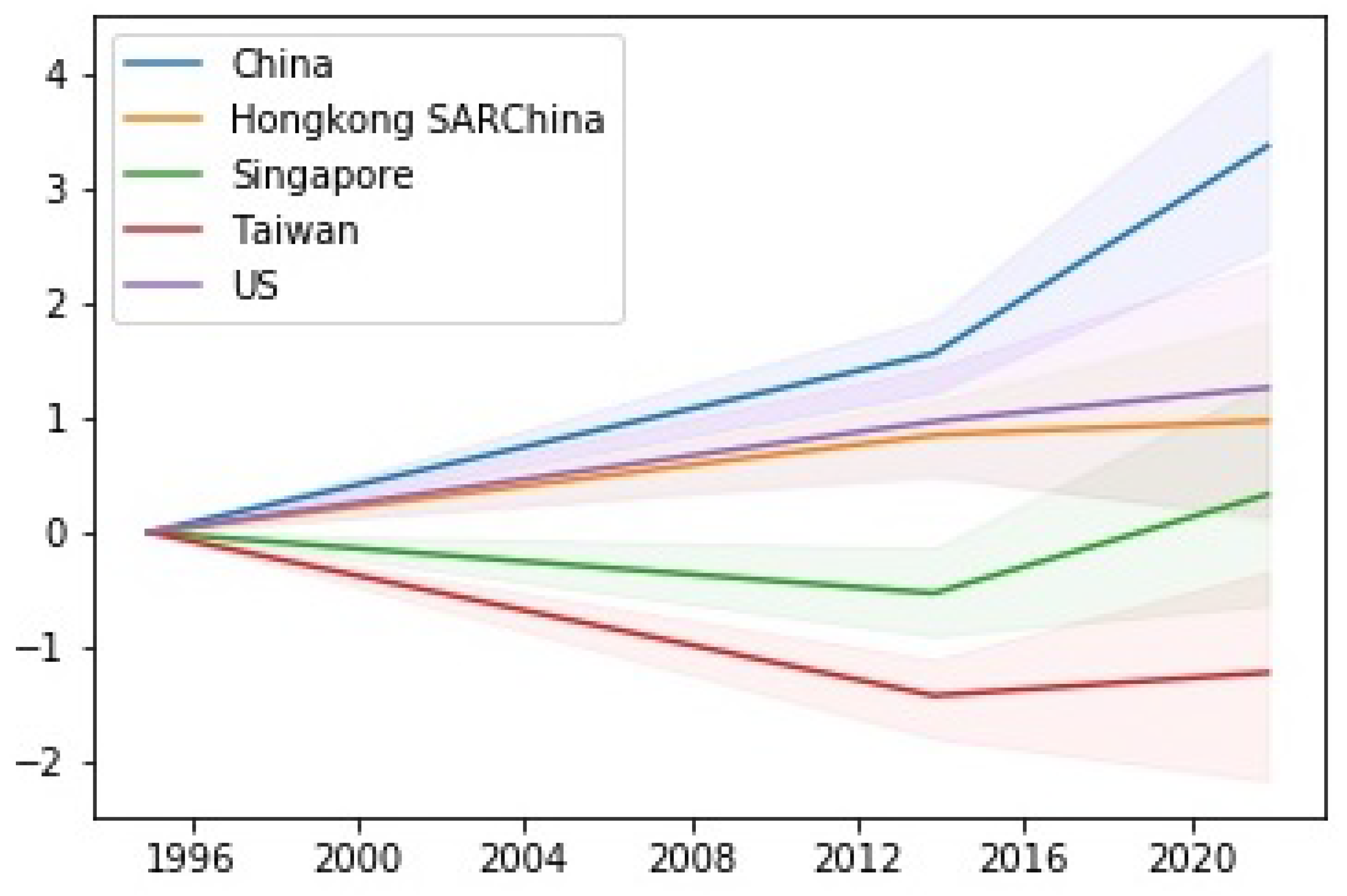
Compared to the results in Table 3, we do not see any notable differences among the intercept estimates in Table 9, except that Intercept (I) is insignificant and Intercept (II) is significantly negative for all countries. As for the slope of the trend, Slope (I) is no longer significant for Singapore and Taiwan and Slope (II, UNESCO) is not significant for Hong Kong. We can also identify these facts from Figure 5. All in all, the sake exported from Nada follows a trend similar to the whole country. Table 10 presents the posterior statistics of coefficients of economic variables. They are comparable to the results in Table 4. Monthly seasonal effects in Table 11 show a one-month lag to the whole country as shown in Table 5. While the seasonal upward movement in export shipments begins in October for the whole country, it starts in November for the Nada region because the Nada region has older breweries that start brewing later. A milder climate in this region also causes the arrival of winter behind much cooler regions (The Nada region is located in a warmer southern part of Japan, while most other sake brewing regions are located in a much cooler northern part of Japan). As a result, breweries in the Nada region must delay the starting date of sake brewing until the temperature becomes sufficiently low.

4.2. Estimation Results of Export Unit Values in Nada

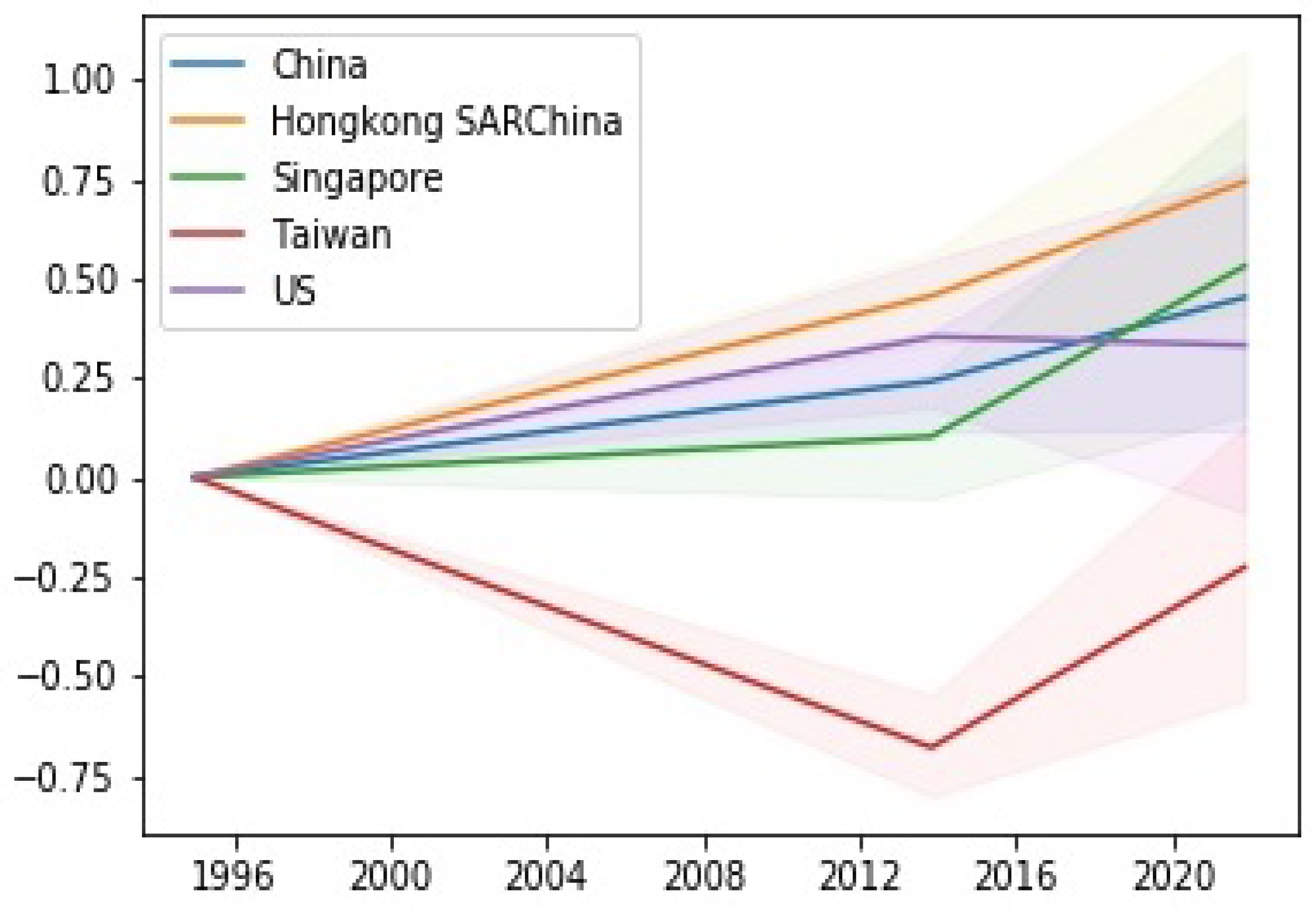
Next, we estimated panel data regression models of the unit value of sake exports from the Nada region. The posterior statistics on trends, coefficients of economic variables, and monthly seasonal effects are shown in Table 12, Table 13 and Table 14, Figure 6, respectively. As for the trend and the impacts of economic variables, we see no clear differences between the Nada region and the whole country. As for the monthly seasonal effects, they almost disappear except for June (Model I and II) and August (Model I). This is because sake breweries in the Nada region tend to prioritize quantity over quality. They do not differentiate their products so much and tend to prioritize the stable supply of their products with fixed prices throughout the year. Unlike small and medium-sized enterprises (SMEs), large breweries do not emphasize entering their products into competition as do small and medium-sized companies, but rather focus on producing inexpensive products with a high degree of productivity.

4.3. Estimation Results of Export Volumes in the Other Area

For the last empirical analysis in this section, we estimated panel data regression models for sake exports from the other regions in Japan. While we have just analyzed sake exports by large firms in the Nada region, it would be fair to say that it is an analysis of small and medium-sized enterprises (SMEs) in the sake brewing industry since large firms are concentrated in the Nada region. The posterior statistics of trends, coefficients of economic variables and monthly seasonal effects in the volume model are shown in Table 15, Table 16 and Table 17 while the corresponding posterior statistics in the unit value model are shown in Table 18, Table 19 and Table 20.
The results of the volume model in Table 15 and Figure 7 are comparable to those in Table 3 and Figure 3, though they show that SMEs are more successful in exporting sake to Singapore and Taiwan because the trends of these countries in Table 15 are steeper than Table 3.
As for economic variables, NER is insignificant for both models in Table 16. This indicates that the impact of exchange rate fluctuations upon the sake exports by SMEs were ambiguous in the sample period.
The seasonal effects are shown in Table 17. This finding is consistent with our conjecture on why seasonal fluctuations appear in sake exports. If the monthly seasonal effects in sake exports are mainly caused by supply-side constraints, they must be more evident for SMEs that lack resources for production and less evident for large firms that have plenty of resources. Thus, the difference in seasonal fluctuations between the Nada region and the other regions reinforces our conjecture.

4.4. Estimation Results of Export Unit Values in the Other Area

As for the unit value model, trends of sake exports by SMEs are close to those of the whole country as shown in Table 18 and Figure 8. It can be seen that sake has become more upscale since the UNESCO registration in all countries except the United States.
It should be noted that sake brewed by SMEs is not affected by the exchange rate in terms of volume in Table 16, but in terms of unit value in Table 19. Exchange rates have a positive impact on both Model I and Model II. This may indicate that there is still room for price hikes and upscaling with regard to products exported by SMEs.
As for the monthly seasonal effects in the unit value model, compared to breweries in the Nada region, they tend to export high-end sake at different times of the year. March, April, and July have a higher impact than January. This is because, after finishing brewing sake for the competition in January, SMEs start entering their sake in the various competitions in February. The results of the competitions are often available between March and July, depending on the type of competition. If a product wins an award at this time, it sells at a higher price as an award-winning product, and this activity is likely to have an impact. Unit values will rise again from early fall onward for the same reasons as the whole country.
Based on findings in this study, it is now clear that there are significant differences in export activities between regions when it comes to sake. It can be said that this study showed the heterogeneity between two types of regions in Japan. For instance, there are some differences between volume trends. Large companies in Nada had a larger impact on the Chinese market than SMEs in the other areas while there is a reverse result in Hong Kong. In unit value trends, large companies made a great recovery in Taiwan market after the UNESCO registration. For the macroeconomic effect, the unit value of SMEs are supported by QQE because it has a significant impact. In the last section, from differences of monthly effects, we can argue that in regions like Nada with a high concentration of large companies and capital, priority is given to brewing stable quantities rather than raising prices, whereas in regions occupied largely by SMEs, brewing high value-added products is required because of the consideration for winning prizes such as Annual Japan Sake Awards.

5. Conclusions

In recent years, sake has been actively exported overseas; however, extant research has not investigated the factors involved. This study analyzed the unbalanced panel of each country using hierarchical Bayesian modeling. As a result, it was confirmed that the registration of Japanese cuisine as an intangible cultural heritage by UNESCO significantly impacted sake exports to some countries. We also confirmed that shipment volume and unit price were related to prices in each country. Furthermore, shipment volume and unit price may differ depending on the season. Additionally, when the data were analyzed separately by company size, it was confirmed that there was little reaction to the unit price in regions with a high concentration of large companies, while in regions with scattered small and medium-sized companies, the unit price was greatly affected by the exchange rate. Our studies can provide some implications for sake breweries and Japanese governments. Overall, the UNESCO registration has boosted exports, especially in China and Hong Kong, which are expected to develop more than ever before. Taiwan and Singapore are the second most attractive markets after China and Hong Kong, given that their growth trends, which were previously negative or close to zero, have improved since UNESCO registration. On the other hand, the export market in the USA is now showing a certain degree of maturity. For the Japanese government, it should be noted that their QQE had a positive impact on exports of SMEs. For large companies, the Japanese government should support them in Taiwan and Singapore, which have still negative trends after the UNESCO registration. Sake exports will continue to grow, and the Japanese government has also made it clear since preparing the 2020 budget that it will invest massive subsidies in sake exports. We hope our research will help businesses currently exporting or considering exporting in the future and the governments supporting them.

Author Contributions

Project administration, investigation, data curation, and writing—original draft preparation, W.S.; software, formal analysis, and resources, M.N.; validation, and supervision, T.N.; conceptualization, and visualization, W.S. and M.N.; writing—review and editing, and funding acquisition, M.N. and T.N.; methodology, W.S., M.N. and T.N. All authors have read and agreed to the published version of the manuscript.

Funding

This research was funded by JSPS KAKENHI Grant Numbers JP23K18819, JP20H00088.

Institutional Review Board Statement

Not applicable.

Informed Consent Statement

Not applicable.

Data Availability Statement

This article includes the data presented in the study.

Conflicts of Interest

The authors declare no conflicts of interest.

Appendix A. Derivation of Conditional Posterior Distribution of Parameters

Appendix A.1. Conditional Posterior Distribution of δ

The conditional posterior distribution of δ is
p ( δ | D , θ δ ) exp 1 2 σ ϵ 2 ( y Z δ ) ( y Z δ ) + ( δ μ ) Σ 1 ( δ μ ) ,
with likelihood (4) and prior distribution (6). We apply the square completion formula, then we obtain (“Constant” means a term that does not depend on δ)
σ ϵ 2 ( y Z δ ) ( y Z δ ) + ( δ μ ) Σ 1 ( δ μ ) = δ σ ϵ 2 Z Z + Σ 1 δ 2 σ ϵ 2 Z y + Σ 1 μ δ + Constant = δ σ ϵ 2 Z Z + Σ 1 1 σ ϵ 2 Z y + Σ 1 μ σ ϵ 2 Z Z + Σ 1 × δ σ ϵ 2 Z Z + Σ 1 1 σ ϵ 2 Z y + Σ 1 μ + Constant .
The conditional posterior distribution of Equation (A1) is
p ( δ | D , θ δ ) exp [ 1 2 δ σ ϵ 2 Z Z + Σ 1 1 σ ϵ 2 Z y + Σ 1 μ σ ϵ 2 Z Z + Σ 1 × δ σ ϵ 2 Z Z + Σ 1 1 σ ϵ 2 Z y + Σ 1 μ ] .
This is equivalent to the probability density function of the distribution in Equation (12).

Appendix A.2. Conditional Posterior Distribution of μγj

The conditional posterior distribution of μ γ j ( j { 1 , , K } ) is
p ( μ γ j | D , θ μ γ j ) exp i = 1 N ( γ i j μ γ j ) 2 2 σ γ j 2 ( μ γ j φ γ ) 2 2 τ γ 2 exp 1 2 σ γ j 2 N + τ γ 2 μ γ j 2 2 σ γ j 2 i = 1 N γ i j + τ γ 2 φ γ μ γ j exp 1 2 σ γ j 2 N + τ γ 2 μ γ j σ γ j 2 i = 1 N γ i j + τ γ 2 φ γ σ γ j 2 N + τ γ 2 2 ,
from Equations (8) and (9). This is equivalent to the probability density function of the distribution in Equation (13).

Appendix A.3. Conditional Posterior Distributions of σ γ j 2 and ξγj

The conditional posterior distribution of σ γ j 2 ( j { 1 , , K } ) is
p ( σ γ j 2 | D , θ σ γ j 2 , ξ γ j ) ( σ γ j 2 ) N 2 exp i = 1 N ( γ i j μ γ j ) 2 2 σ γ j 2 × ( σ γ j 2 ) 1 2 + 1 exp 1 ξ γ j σ γ j 2 ( σ γ j 2 ) N + 1 2 + 1 exp 1 2 i = 1 N ( γ i j μ γ j ) 2 + ξ γ j 1 σ γ j 2 ,
given the latent variable ξ γ j from Equations (8) and (16). This is equivalent to the probability density function of the distribution of σ γ 2 in Equation (14). Whereas, the conditional posterior distribution of ξ γ j is obtained as
p ( ξ γ j | σ γ j 2 ) ξ γ j 1 2 ( σ γ j 2 ) 1 2 + 1 exp 1 ξ γ j σ γ j 2 × ξ γ j 1 2 + 1 exp 1 s γ 2 ξ γ j ξ γ j ( 1 + 1 ) exp σ γ j 2 + s γ 2 ξ γ j .
This is also equivalent to the probability density function of the distribution of ξ γ j in Equation (14).

Appendix A.4. Conditional Posterior Distribution of σ ϵ 2 and ξϵ

The conditional posterior distribution of σ ϵ 2 is
p ( σ ϵ 2 | D , θ σ ϵ 2 ) ( σ ϵ 2 ) T 2 exp i = N t = 1 T i e i t 2 2 σ ϵ 2 × ( σ ϵ 2 ) 1 2 + 1 exp 1 ξ ϵ σ ϵ 2 ( σ ϵ 2 ) T + 1 2 + 1 exp 1 2 i = 1 N t = 1 T i e i t 2 + ξ ϵ 1 σ ϵ 2 ,
from Equations (5) and (16). This is equivalent to the probability density function of the distribution in Equation (15). Whereas, the conditional posterior distribution of ξ ϵ in Equation (15) is derived by replacing σ γ j 2 and s γ 2 by σ ϵ 2 and s ϵ 2 in Equation (A5), respectively.

References

  1. Sake Reports in March 2022 (Sake no Shiori Reiwa 4 Nendo 3 Gatsu). 2022. Available online: https://www.nta.go.jp/taxes/sake/shiori-gaikyo/shiori/2022/index.htm (accessed on 28 April 2024).
  2. Shinato, T.; Kato, K. A Study on the Expansion of Sake Exports: A Comparative Study with the Globalization of French Wine (Ninonshu No Yushutu Kakudai Ni Kakaru Ichikousatu—Furansuwain Tono Hikaku Kosatsu). Bull. Soc. E Fr. Jpn. Gest. 2020, 37, 14–30. [Google Scholar]
  3. Kishi, Y. Global development of sake and its global consumption - Developing sales channels in line with wine consumption styles. (Nihonshu No Gurobaru Tenkai Sono Gurobaru Na Shohi—Wain No Shohi Sutairu Ni Awaseta Hanro Kaitaku). J. Home. Econ. Jpn. 2018, 69, 830–835. [Google Scholar]
  4. Handbook of Japanese Sake Export to China. 2018. Available online: https://www.jetro.go.jp/ext_images/_Reports/02/79e096522d9b221f/cn_reports.pdf (accessed on 28 April 2024).
  5. Handbook of Japanese Sake Export to US. 2018. Available online: https://www.jetro.go.jp/ext_images/_Reports/02/2018/e6c0d0ebdd040e46/us_reports.pdf (accessed on 28 April 2024).
  6. Fujishiro, N. U.S. Sake Market Expansion and Factors behind the rise in export unit price (Beikoku no Seishu Shijo Kakudai to Yushutu Tanak Josho no Youin. In Proceedings of the 8th Marketing Conference 2019, Tokyo, Japan, 26 November 2019; pp. 319–327. [Google Scholar]
  7. Bouët, A.; Emlinger, C.; Lamani, V. What Determines Exports of Luxury Products? The Case of Cognac. J. Wine Econ. 2017, 66, 37–58. [Google Scholar] [CrossRef]
  8. Bargain, O. French Wine Exports to China: Evidence from Intra-French Regional Diversification and Competition. J. Wine Econ. 2020, 15, 134–162. [Google Scholar] [CrossRef]
  9. Cardebat, J.; Figuet, J. The Impact of Exchange Rates on French Wine Exports. J. Wine Econ. 2019, 14, 71–89. [Google Scholar] [CrossRef]
  10. Candau, F.; Deisting, F.; Schlick, J. How income and crowding effects influence the world market for French wines. World Econ. 2017, 40, 963–977. [Google Scholar] [CrossRef]
  11. Capitello, R.; Agnoli, L.; Begalli, D. Chinese import demand for wine: Evidence from econometric estimations. J. Wine Res. 2015, 26, 115–135. [Google Scholar] [CrossRef]
  12. Fontagné, L.; Hatte, S. European High-End Products in International Competition. Working Paper. 2013. Available online: https://www.parisschoolofeconomics.eu/IMG/pdf/wp37-gmond-europe-competition-nov2013.pdf (accessed on 28 April 2024).
  13. Mitchell, L. Demand for Wine and Alcoholic Beverages in the European Union: A Monolithic Market? J. Wine Econ. 2016, 11, 414–435. [Google Scholar] [CrossRef]
  14. Nelson, J.P. Robust demand elasticities for wine and distilled spirits: Meta-analysis with corrections for outliers and publication bias. J. Wine Econ. 2013, 12, 117–148. [Google Scholar] [CrossRef]
  15. Fogarty, J. The demand for beer, wine and spirits: A survey of the literature. J. Econ. Sur. 2010, 24, 428–478. [Google Scholar] [CrossRef]
  16. Lombardi, P.; Bianco, A.D.; Roberto, F.; Caraccioloa, F.; Cembalo, L. Development and trade competitiveness of the European wine sector: A gravity analysis of intra-EU flows. Wine Econ. Pol. 2016, 8, 50–59. [Google Scholar] [CrossRef]
  17. Bargain, O.; Cardebat, J.M.; Chiappini, R.; Laffitte, C. Long-term prospects of the international wine trade. J. Wine Econ. 2018, 13, 442–450. [Google Scholar] [CrossRef]
  18. Connolly, C.; Graziano, M.; McDonnell, A.; Steinbach, S. In Cervisia Veritas: The impact of repealing Sunday blue laws on alcohol sales and retail competition. J. Wine Econ. 2023, 18, 312–323. [Google Scholar] [CrossRef]
  19. Hart, J.; Alston, J.M. Evolving Consumption Patterns in the U.S. Alcohol Market: Disaggregated Spatial Analysis. J. Wine Econ. 2020, 8, 159–188. [Google Scholar] [CrossRef]
  20. Gelman, A. Prior Distributions for Variance Parameters in Hierarchical Models. Bayes. Anal. 2010, 1, 515–534. [Google Scholar]
  21. Schmidt, D.F.; Makalic, E. A Simple Sampler for the Horseshoe Estimator. IEEE Sig. Proc. Let. 2016, 23, 179–182. [Google Scholar]
  22. Yu, Y.; Meng, X.L. To Center or Not to Center: That is Not the Question—An Ancillarity-Sufficiency Interweaving Strategy (ASIS) for Boosting MCMC Efficiency. J. Comp. Graph Stat. 2011, 20, 531–570. [Google Scholar] [CrossRef]
  23. Saito, W.; Nakatsuma, T. Hierarchical Bayesian hedonic regression analysis of Japanese rice wine: Is the price right? Int. J. Wine Bis. Res. 2023, 35, 256–277. [Google Scholar] [CrossRef]
  24. Akiyama, H. An Overview of Sake: Present and Past. In Sake; Iwanami Shoten: Tokyo, Japan, 1994; pp. 11–14. [Google Scholar]
Figure 1. Japanese rice wine, sake. (The picture was obtained from the Japanese Sake and Shochu Makers Association, https://japansake.or.jp/sake/en/ (accessed on 2 August 2024)).
World 05 00036 g001
Figure 2. Japanese sake export (For y-axis labels, “Thousand KL” means thousand kiloliter, “Million JPY” means million Japanese Yen, and “JPY per Liter” means Japanese yen per liter).
World 05 00036 g002
Figure 3. Export volume trends.
World 05 00036 g003
Figure 4. Export unit value trends.
World 05 00036 g004
Figure 5. Export volume trends, Nada region.
World 05 00036 g005
Figure 6. Export unit value trends, Nada region.
World 05 00036 g006
Figure 7. Export volume trends, other area.
World 05 00036 g007
Figure 8. Export unit value trends, other areas.
World 05 00036 g008
Table 1. Descriptive statistics.
VariablesMeanStdMaxMinN
Unit (All)0.8290.1891.1930.3591601
Unit (China)0.6040.2991.7680.176313
Unit (Hong Kong SAR China)0.9770.6643.4050.301323
Unit (Singapore)0.9080.4002.7970.401323
Unit (Taiwan)0.3830.1581.1080.184319
Unit (US)0.8290.1891.1930.359323
CPI (All)113.07451.856278.80264.3001601
CPI (China)102.5873.210120.70097.900313
CPI (Hong Kong SAR China)78.96311.943102.20064.300323
CPI (Singapore)85.77811.342104.43970.681323
CPI (Taiwan)88.4777.082101.24075.040319
CPI (US)208.93534.532278.802150.900323
Exchange (All)96.72212.821124.80959.5761601
Exchange (China)82.53310.807101.50459.576313
Exchange (Hong Kong SAR China)107.6699.177123.48592.900323
Exchange (Singapore)90.9378.558104.24979.548323
Exchange (Taiwan)105.2017.383124.80993.225319
Exchange (US)96.9358.464115.33381.484323
Quantity (All)152,700156,92010,579,0001461601
Quantity (China)112,970168,590807,200146313
Quantity (Hong Kong SAR China)114,76058,597363,65026,647323
Quantity (Singapore)31,68917,509114,7006060323
Quantity (Taiwan)200,320141,8301,025,7001620319
Quantity (US)303,110164,9201,057,90053,207323
Price (All)126,790174,0401,240,5002131601
Price (China)107,760211,2601,240,500213313
Price (Hong Kong SAR China)143,400179,0001,141,40010,207323
Price (Singapore)33,49734,896228,9303208323
Price (Taiwan)73,07350,845325,4201425319
Price (US)274,980192,8901,225,70026,308323
Table 2. Model specifications.
Model IModel II
Constant TermCountry-specificCountry-specific
Time TrendCountry-specificCountry-specific
U N E S C O d u m m y ×(None)Country-specific
U N E S C O t r e n d ×(None)Country-specific
Unit CommonCommon
CPI CommonCommon
NER CommonCommon
Seasonal DummyCommonCommon
Table 3. Country-specific trends (export volume).
ChinaHong KongSingaporeTaiwanUS
Intercept (I)0.4173.388 **2.3354.473 **3.268
(1.589)(1.536)(1.497)(1.575)(1.710)
Intercept (II)−1.3631.8510.9763.0801.196
(2.006)(1.976)(1.902)(2.003)(2.175)
Intercept (II, UNESCO)0.194−0.310 **0.0450.415−0.122
(0.108)(0.118)(0.109)(0.105)(0.107)
Slope (I)0.014 **0.004 **0.002 **−0.001 **0.003 **
(0.000)(0.000)(0.000)(0.000)(0.000)
Slope (II)0.013 **0.005 **0.001−0.005 **0.004 **
(0.000)(0.000)(0.001)(0.001)(0.000)
Slope (II, UNESCO)0.014 **0.004 **0.009 **0.012 **−0.001
(0.001)(0.001)(0.001)(0.001)(0.001)
Table 4. Impacts of economic variables (export volume).
Unit CPI NER
Model I−0.204 **1.201 **0.443 **
(0.061)(0.282)(0.188)
Model II−0.630 **1.925 **0.024
(0.062)(0.344)(0.230)
Table 5. Monthly seasonal effects (export volume).
FebruaryMarchAprilMayJuneJuly
Model I0.162 **0.242 **0.173 **0.0540.025−0.010
(0.058)(0.058)(0.056)(0.058)(0.059)(0.058)
Model II0.152 **0.237 **0.170 **0.0630.0520.016
(0.055)(0.053)(0.055)(0.054)(0.054)(0.054)
AugustSeptemberOctoberNovemberDecember
Model I−0.0780.0530.166 **0.230 **0.341 **
(0.057)(0.057)(0.056)(0.058)(0.058)
Model II−0.0700.0620.181 **0.236 **0.357 **
(0.055)(0.055)(0.054)(0.055)(0.058)
Table 6. Country-specific trends (export unit value).
ChinaHong KongSingaporeTaiwanUS
Intercept (I)−8.353 **−7.886 **−7.400 **−8.310 **−8.200 **
(0.636)(0.616)(0.602)(0.630)(0.700)
Intercept (II)−6.07 **−5.510 **−5.105 **−5.807 **−5.961 **
(0.814)(0.803)(0.775)(0.814)(0.885)
Intercept (II, UNESCO)−0.068−0.132 **0.0700.107 **0.028
(0.044)(0.048)(0.045)(0.043)(0.044)
Slope (I)0.003 **0.005 **0.002 **0.001 **0.000
(0.000)(0.000)(0.000)(0.000)(0.000)
Slope (II)0.013 **0.005 **0.001−0.005 **0.004 **
(0.000)(0.000)(0.001)(0.001)(0.000)
Slope (II, UNESCO)0.005 **0.004 **0.004 **0.006 **−0.002 **
(0.001)(0.001)(0.001)(0.001)(0.001)
Table 7. Impacts of economic variables (export unit value).
CPI NER
Model I1.141 **0.398 **
(0.115)(0.078)
Model II0.996 **0.039
(0.139)(0.094)
Table 8. Monthly seasonal effects (export unit value).
FebruaryMarchAprilMayJuneJuly
Model I−0.01800050.0090.0260.091**0.084 **
(0.024)(0.024)(0.025)(0.025)(0.024)(0.024)
Model II−0.0200.0200.0060.0240.008 **0.008 **
(0.022)(0.022)(0.022)(0.022)(0.022)(0.022)
AugustSeptemberOctoberNovemberDecember
Model I0.052 **0.053 **0.067 **0.055 **0.076 **
(0.024)(0.025)(0.024)(0.024)(0.024)
Model II0.046 **0.047 **0.062 **0.048 **0.070 **
(0.022)(0.022)(0.022)(0.023)(0.022)
Table 9. Country-specific trends (export volume, Nada region).
ChinaHong KongSingaporeTaiwanUS
Intercept (I)−3.412−0.750−1.530−0.564−1.550
(2.010)(1.947)(1.902)(1.994)(2.178)
Intercept (II)−8.031 **−5.180 **−5.711 **−4.850 **−7.101 **
(2.571)(2.530)(2.442)(2.563)(2.796)
Intercept (II, UNESCO)1.065 **−0.387 **0.010.684 **0.167
(0.141)(0.155)(0.145)(0.138)(0.141)
Slope (I)0.012 **0.002 **0.001 0.001 0.005 **
(0.001)(0.001)(0.001)(0.000)(0.001)
Slope (II)0.006 **0.004 **−0.002 **−0.006 **0.004 **
(0.001)(0.001)(0.001)(0.001)(0.000)
Slope (II, UNESCO)0.012 **−0.0020.011 **0.008 **−0.001
(0.002)(0.002)(0.002)(0.002)(0.002)
Table 10. Impact of economic variables (export volume, Nada region).
Unit CPI NER
Model I−0.540 **1.408 **0.960 **
(0.064)(0.361)(0.246)
Model II−0.940 **2.800 **0.551
(0.066)(0.448)(0.230)
Table 11. Monthly seasonal effects (export volume, Nada region).
FebruaryMarchAprilMayJuneJuly
Model I0.172 **0.270 **0.156 **0.1410.015 0.020
(0.076)(0.077)(0.076)(0.078)(0.077)(0.076)
Model II0.612 **0.260 **0.137 **0.156 **0.0210.034
(0.070)(0.070)(0.070)(0.071)(0.071)(0.070)
AugustSeptemberOctoberNovemberDecember
Model I 0.041 0.0210.0880.200 **0.362 **
(0.067)(0.076)(0.075)(0.076)(0.075)
Model II 0.021 0.0330.1060.193 **0.364 **
(0.069)(0.070)(0.070)(0.071)(0.070)
Table 12. Country-specific trends (export unit value, Nada region).
ChinaHong KongSingaporeTaiwanUS
Intercept (I)−6.364 **−6.059 **−5.630 **−6.506 **−6.518 **
(0.790)(0.762)(0.746)(0.681)(0.855)
Intercept (II)−4.081 **−3.520 **−3.289 **−3.810 **−4.180 **
(1.018)(1.001)(0.966)(1.015)(1.107)
Intercept (II, UNESCO)0.370 **−0.013−0.0080.224 **0.214 **
(0.053)(0.059)(0.054)(0.053)(0.054)
Slope (I)0.002 **0.003 **0.001 ** 0.000 0.002 **
(0.000)(0.000)(0.000)(0.000)(0.000)
Slope (II)0.013 **0.005 **0.001−0.005 **0.004 **
(0.000)(0.000)(0.001)(0.001)(0.000)
Slope (II, UNESCO)0.0010.0010.004 **0.008 **−0.002 **
(0.001)(0.001)(0.001)(0.001)(0.001)
Table 13. Impacts of economic variables (export unit value, Nada region).
CPI NER
Model I0.643 **0.468 **
(0.143)(0.095)
Model II0.728 **−0.131
(0.177)(0.115)
Table 14. Monthly seasonal effects (export unit value, Nada region).
FebruaryMarchAprilMayJuneJuly
Model I 0.020 0.012 0.004 0.0380.061 **0.050
(0.030)(0.030)(0.030)(0.030)(0.030)(0.030)
Model II 0.020 0.015 0.001 0.0370.057 **0.048
(0.025)(0.026)(0.027)(0.027)(0.027)(0.026)
AugustSeptemberOctoberNovemberDecember
Model I0.073 **0.0470.0620.0150.042
(0.029)(0.030)(0.029)(0.029)(0.029)
Model II0.0700.0440.0610.0120.035
(0.026)(0.027)(0.026)(0.027)(0.027)
Table 15. Country-specific trends (export volume, other areas).
ChinaHong KongSingaporeTaiwanUS
Intercept (I) 12.037 ** 6.293 6.310 5.976 5.260
(3.527)(3.430)(3.341)(3.506)(3.821)
Intercept (II) 11.177 ** 4.771 4.540 4.060 4.183
(4.707)(4.647)(4.470)(4.704)(5.115)
Intercept (II, UNESCO) 1.225 ** 0.610 **0.3440.478 0.312
(0.277)(0.297)(0.270)(0.266)(0.270)
Slope (I)0.035 **0.019 **0.011 **0.007 **0.005 **
(0.001)(0.001)(0.001)(0.000)(0.001)
Slope (II)0.040 **0.020 **0.082 **0.0010.007 **
(0.001)(0.001)(0.001)(0.001)(0.002)
Slope (II, UNESCO)0.010 **0.011 **0.013 **0.017 ** 0.006
(0.004)(0.004)(0.004)(0.004)(0.004)
Table 16. Impacts of economic variables (export volume, other areas).
Unit CPI NER
Model I−2.347 **2.518 **0.481
(0.103)(0.642)(0.442)
Model II−2.572 **2.771 ** 0.003
(0.110)(0.830)(0.563)
Table 17. Monthly seasonal effects (export volume, other areas).
FebruaryMarchAprilMayJuneJuly
Model I0.2000.271 **0.311 **0.1490.294 **0.125
(0.141)(0.140)(0.139)(0.140)(0.138)(0.142)
Model II0.1880.267 **0.302 **0.1430.302 **0.138
(0.134)(0.132)(0.136)(0.135)(0.136)(0.135)
AugustSeptemberOctoberNovemberDecember
Model I 0.074 0.2270.402 **0.404 **0.543 **
(0.138)(0.140)(0.138)(0.138)(0.140)
Model II 0.078 0.2130.389 **0.398 **0.546 **
(0.135)(0.133)(0.135)(0.135)(0.134)
Table 18. Country-specific trends (export unit value, other area).
ChinaHong KongSingaporeTaiwanUS
Intercept (I) 7.910 ** 8.046 ** 7.294 ** 8.352 ** 8.107 **
(0.889)(0.863)(0.844)(0.883)(0.964)
Intercept (II) 8.691 ** 8.890 ** 7.995 ** 9.077 ** 9.181 **
(1.232)(1.217)(1.171)(1.231)(1.341)
Intercept (II, UNESCO) 0.045 0.250 **0.138 **0.158 ** 0.033
(0.064)(0.070)(0.065)(0.062)(0.065)
Slope (I)0.002 **0.006 **0.002 **0.002 **0.000
(0.000)(0.000)(0.000)(0.000)(0.000)
Slope (II)0.001 **0.006 **0.0000.001 **0.000
(0.000)(0.000)(0.000)(0.000)(0.000)
Slope (II, UNESCO)0.007 **0.0020.004 **0.003 ** 0.002
(0.001)(0.001)(0.001)(0.001)(0.001)
Table 19. Impact of economic variables (export unit value, other areas).
CPI NER
Model I1.100 **0.484 **
(0.158)(0.108)
Model II1.338 **0.445 **
(0.209)(0.140)
Table 20. Monthly seasonal effects (export unit value, other area).
FebruaryMarchAprilMayJuneJuly
Model I 0.023 0.0200.0060.0220.0102 **0.122 **
(0.034)(0.034)(0.035)(0.035)(0.035)(0.034)
Model II 0.024 0.0180.0030.0220.099 **0.120 **
(0.032)(0.032)(0.032(0.032)(0.033)(0.032)
AugustSeptemberOctoberNovemberDecember
Model I0.080 **0.0370.0290.0600.075 **
(0.034)(0.034)(0.034)(0.034)(0.033)
Model II0.075 **0.0310.0230.0520.070 **
(0.032)(0.031)(0.032)(0.032)(0.032)
Disclaimer/Publisher’s Note: The statements, opinions and data contained in all publications are solely those of the individual author(s) and contributor(s) and not of MDPI and/or the editor(s). MDPI and/or the editor(s) disclaim responsibility for any injury to people or property resulting from any ideas, methods, instructions or products referred to in the content.