A Complete System for Automated Semantic–Geometric Mapping of Corrosion in Industrial Environments

Abstract

Corrosion, a naturally occurring process leading to the deterioration of metallic materials, demands diligent detection for quality control and the preservation of metal-based objects, especially within industrial contexts. Traditional techniques for corrosion identification, including ultrasonic testing, radiographic testing, and magnetic flux leakage, necessitate the deployment of expensive and bulky equipment on-site for effective data acquisition. An unexplored alternative involves employing lightweight, conventional camera systems and state-of-the-art computer vision methods for its identification. In this work, we propose a complete system for semi-automated corrosion identification and mapping in industrial environments. We leverage recent advances in three-dimensional (3D) point-cloud-based methods for localization and mapping, with vision-based semantic segmentation deep learning techniques, in order to build semantic–geometric maps of industrial environments. Unlike the previous corrosion identification systems available in the literature, which are either intrusive (e.g., electrochemical testing) or based on costly equipment (e.g., ultrasonic sensors), our designed multi-modal vision-based system is low cost, portable, and semi-autonomous and allows the collection of large datasets by untrained personnel. A set of experiments performed in relevant test environments demonstrated quantitatively the high accuracy of the employed 3D mapping and localization system, using a light detection and ranging (LiDAR) device, with less than $0.05$ m and $0.02$ m average absolute and relative pose errors. Also, our data-driven semantic segmentation model was shown to achieve $70\%$ precision in corrosion detection when trained with our pixel-wise manually annotated dataset.

1. Introduction

Corrosion refers to the chemical or electrochemical degradation of materials due to reactions with environmental elements such as moisture, oxygen, or industrial chemicals. This degradation alters not only the surface of the material, geometry, and structure but also affects the functional integrity of structural components over time. This is a major problem that degrades metallic surfaces, which are ubiquitous in man-made constructions. Its identification and mitigation have significant socio-economic impacts across various industries, contributing to the maintenance and longevity of infrastructures, such as bridges, pipelines, and buildings, to name a few, reducing the frequency of reconstruction projects and associated costs [1]. Early and accurate identification of corrosion allows for timely intervention and maintenance, preventing costly repairs and replacements and reducing downtime in industries such as oil and gas, aerospace, and manufacturing, leading to increased productivity and financial savings [2]. Corrosion in metal-made infrastructures can lead to leaks and spills, causing environmental pollution. Timely identification helps prevent such incidents, preserving ecosystems and minimizing the environmental impact [3]. Also, corrosion-related failures can compromise the safety of structures and equipment. Identifying and addressing corrosion hazards enhance workplace safety and reduce the risk of accidents and injuries in operation, potentially leading to softer workplace health and safety insurance policies with lower premiums for well-maintained and corrosion-free assets [1].

Among the leading-edge technologies for identifying corrosion, magnetic flux leakage, ultrasonic testing, and remote visual inspection stand out. Although magnetic flux leakage provides highly accurate solutions, its deployment is expensive, challenging, and necessitates skilled and trained human operators for successful operation. However, the current process of inspecting offshore assets using visual inspection technologies and evaluating where to conduct maintenance and repairs is a highly manual and laborious task. First, inspectors are required to traverse the asset and record and track a large number of images of corroded elements, which are manually labeled in a coarse manner. For some structures, such as offshore wind turbines, autonomous or remotely operated robots are being deployed to cover hard to reach areas and perform data collection; however, automated data analysis methods are still inaccurate, lacking in production environments, and hence, human experts are still required to perform this task [4]. Also, industrial assets can be multi-story, multi-platform metal structures, naturally resulting in the collection of large datasets, which may be unfeasible to transmit via satellite connections, for instance, in remote offshore locations. Additionally, the nature of industrial assets, as well as various safety and security concerns surrounding them, add challenges to performing the inspection task.

After the data collection procedure, the collected datasets undergo manual review by experts, evaluating the severity of the corrosion, and thus which structures require maintenance and for which maintenance can be postponed. Some structures are more critical than others to maintain, for the sake of asset operation and safety. As part of this review, most of the time is spent resolving where a given image was recorded and identifying the specific location of the corroded structure. This process involves the development of maintenance work packages. Within these packages, structures identified as critically corroded are designated for maintenance, repair, or replacement. These tasks may extend over several months, whether carried out on-site or, in the case of mobile offshore platforms, at a dry dock.

To alleviate some of the challenges posed by the manual nature of the current process, we envision a data collection device with the following general properties:

• Portability: Inspectors should be able to easily carry and operate the data collection device in industrial assets during long periods.
• Accuracy: High precision imaging sensors for accurate 3D semantic mapping of corroded assets.
• Autonomy: Intelligent software that should be able to perform mapping, localization, and semantic localization and categorization of industrial assets from sensory data. However, the software may not strictly run online, on the data collection device, but instead offline in a more powerful computational device.

Taking into account the previous properties, we leverage current advances in vision-based semantic segmentation and simultaneous localization and mapping (SLAM) approaches, and the availability of low-cost consumer-grade light detection and ranging (LiDAR) and visual camera systems, to propose a complete geometric–semantic mapping and localization system. We combine highly accurate 3D point cloud data provided by LiDAR, with monocular color vision for robust and precise localization of corrosion spots in 3D. In particular, the main contributions of this work can be summarized as follows:

• Design of a portable, accurate, and autonomous system for detection corrosion based on the integration state-of-the-art technologies.
• Algorithmic design and full prototype implementation of the integrated system.
• Validation and performance evaluation of the automated system in relevant test environments.

The main novelties and benefits of the proposed solution originated in the coordinated integration of technologies allowing for extra degrees of freedom in operational conditions as the system reduces human manual work and allows for multiple online automated simultaneous computations that are not possible in current commercial solutions.

The rest of this article is organized as follows. First, in Section 2, we review the state-of-the-art technologies for positioning and corrosion identification, with a focus on vision-based 3D localization and mapping and semantic segmentation techniques. Second, in Section 3, we describe in detail the proposed system, including design and sensor choices, as well as algorithmic choices. Then, in Section 4, we validate our system and demonstrate its applicability by reporting the results from a set of experiments performed both in an indoor laboratory scenario and in an outdoor offshore environment. Finally, we draw our main conclusions and propose extensions for future work in Section 5.

2. Related Work

In this section, we overview the state-of-the-art methods utilized in our approach, including existing technologies for positioning, corrosion detection, vision-based sensor calibration, localization and mapping, and semantic segmentation techniques.

2.1. Positioning Systems

Multiple positioning technologies exist and have been reported in the literature for multiple purposes. With a focus on offshore positioning cases, industrial positioning, emergency systems, and positioning systems for autonomous systems, the following was concluded.

Technologies such as Ultra-Wide Band (UWB) [5], ultra-sound [6], Wi-Fi [7], and Bluetooth Low-Energy (BLE) [8] can work in indoor settings and are simple to deploy as end-user devices are typically based on tags or small battery-power devices. However, these technologies present also some drawbacks. They normally require a dedicated and complex infrastructure deployment with anchors/routers, wires, and centralized control computers, as well as an accurate calibration process. While in typical industrial settings, such as factory halls, these types of deployments might be feasible, the situation in offshore is more complicated (e.g., in oil/gas platforms). In general, these technologies require a clear line of sight between infrastructure and localization devices to guarantee a correct operation (i.e., at least three visible routers/anchors at all times to be able to perform triangulation), which is difficult in both industrial and offshore scenarios. Moreover, localization based on these technologies does typically not provide heading/orientation information and does not perform well when the localization devices are close to large metal surfaces. The accuracy of these systems in industrial settings typically range from approximately 20 cm for UWB (with some sporadic deviations to more than 1 m in certain conditions) to approximately 1.5 m for Wi-Fi and BLE.

Technologies based on satellite systems such as Global Navigation Satellite System (GNSS)/Real-Time Kinematic (RTK) [9] and Differential Global Positioning Systems (DGPSs) [10] can offer up to cm-level accuracy in industrial and offshore environments (e.g., in offshore windmill inspection applications [4]). However, the applicability of these technologies is limited to areas with a full or partial view of the sky, hence inapplicable in indoor settings [11]. In general, these technologies rely on no infrastructure (e.g., GNSS, where only an end-user device is required) or simple infrastructure (e.g., RTK and DGPS), where a single unit or just a few independent units are typically needed for automatic system calibration/correction.

As an alternative, it is possible to use novel technologies or combinations of technologies that do not rely on external infrastructure [12]. Here, recent advances in Computer Vision (CV) [13] methods for SLAM [14] and Visual-Inertial Odometry (VIO) [15] are at hand, allowing for simultaneous high-precision, real-time, and low-cost state estimation (i.e., tracking), the provisioning of a six degrees of freedom (6 DoF) position, and orientation information and mapping. Of course, all these benefits have some associated limitations that need to be overcome such as the unavailability of unified commercial solutions and more complicated integration setups. Other challenges may include occasional poor performance in featureless areas and the potential need for high computational resources and stability requirements for mobile setups [16]. Sensor fusion strategies (e.g., integration with Inertial Measurement Units (IMUs)) might be of utility to overcome some of the said challenges.

Therefore, to make our proposed solution as universal as possible, relying on external infrastructure or specific conditions is avoided, making it compatible with most of the potential industrial and offshore scenarios. Hence, the last group of novel technologies, and its combination, will be explored.

2.2. Technologies for Corrosion Identification

Identifying corrosion relies on diverse technologies [17] capable of detecting, quantifying, and characterizing corrosion processes in various materials and environments. Commonly employed methods include Ultrasonic Testing (UT) [18], which utilizes high-frequency sound waves for internal and surface defect detection in industries like oil and gas, aerospace, and manufacturing. Eddy Current Testing (ECT) [19] is a method that utilizes electromagnetic induction, being particularly useful for inspecting non-ferrous metals and detecting corrosion under protective coatings. Radiographic Testing (RT) [20] involves X-rays or gamma rays to inspect internal structures, commonly applied in aerospace, construction, and automotive industries.

Electrochemical Techniques (ETs) [21], encompassing methods like impedance spectroscopy and potentiodynamic polarization, study the electrochemical behavior of metals in corrosive environments, providing vital information on corrosion rates and protection effectiveness. Infrared Thermography (IRT) [22], a non-contact method using infrared cameras, is beneficial for inspecting large areas in industries such as building inspection, aerospace, and electrical utilities. Visual Inspection [23], a basic method involving the visual examination of surfaces, is often used alongside other testing methods to assess corrosion severity. Additional technologies like magnetic particle testing [24], acoustic emission testing [25], and scanning electron microscopy [26] also contribute significantly to corrosion identification.

These technologies play a crucial role in preventing material degradation, structural failure, and costly repairs. Our proposed pipeline employs a vision-based deep-learning method, leveraging low-cost camera sensors for accurate and easily deployable results in corrosion assessment.

2.3. Camera and LiDAR Calibration

Camera, LiDAR, and inertial (i.e., IMU) calibration constitutes an essential step in sensor fusion for robotics, autonomous vehicles, and augmented reality applications [27]. This process ensures accurate alignment and synchronization between these sensors. Calibration enables the transformation of measurements from different sensors into a common reference frame, allowing seamless integration of data for robust perception and navigation.

Camera calibration involves determining the intrinsic and extrinsic parameters of a camera, which include focal length, principal point, distortion coefficients, and the transformation (rotation and translation) between the camera and the world coordinate system. The calibration is often performed using a calibration target with known geometric features (typically a checkerboard pattern with known dimensions), and the parameters are estimated by minimizing the re-projection error [28]. A set of algorithms for the calibration of various camera sensors, commonly used in robotics applications (e.g., for precise sensor fusion and localization) can be found in a popular open-source toolbox named Kalibr [29]. These algorithms are not limited to single camera systems and may be used to calibrate multiple cameras (stereo) of various types and IMUs.

LiDAR–camera calibration involves aligning LiDAR data with a camera to ensure the accurate fusion of LiDAR point clouds with the camera. The calibration process determines the transformation matrices between the LiDAR and camera coordinate systems [30]. Calibration, in this case, is typically performed by capturing synchronized data from both sensors while the system undergoes controlled motion. In all cases, optimization techniques, such as non-linear least squares, are used to estimate the transformation matrices holding the intrinsic and extrinsic parameters of the sensors.

2.4. LiDAR-Based Localization and Mapping

LiDAR-based SLAM is an advanced technology that combines data from LiDAR sensors and optionally IMUs to achieve real-time localization and mapping in dynamic environments. LiDAR sensors employ laser beams to measure distances and create detailed three-dimensional (3D) maps of the surroundings, while IMUs, equipped with accelerometers and gyroscopes, capture information about the platform’s acceleration and angular rate. The integration of LiDAR and IMU data enhances the accuracy and robustness of the system, especially in scenarios where GNSS may be unreliable, such as indoor or urban environments.

Approaches for LiDAR-based SLAM involve estimating the precise position and orientation of the sensor apparatus in relation to its surroundings while building a map representation of the environment (typically a point cloud), without prior knowledge of the surroundings. This is achieved through continuous fusion and optimization of LiDAR and, if available, IMU measurements, enabling the system to maintain an accurate and up-to-date understanding of its pose. The integration of these sensors facilitates overcoming challenges like dynamic movements, changes in orientation, and variations in the environment. Loop-closure detection is a crucial technique employed in SLAM for recognizing previously mapped locations and features. Through realigning the matching prior and current observations, accumulated errors in both localization and mapping can be corrected [31].

When a map of the environment is known a priori, SLAM simplifies to a localization problem, in which the goal is to estimate the sensor apparatus pose with respect to the map coordinate system. LiDAR-based SLAM and localization systems are crucial for various applications, including robotics, autonomous vehicles, and augmented reality, where high-precision spatial awareness and real-time localization are paramount. Researchers and engineers continue to refine and develop LiDAR SLAM algorithms to enhance performance, robustness, and adaptability across diverse and challenging scenarios. We overview the most relevant state-of-the-art approaches below.

2.4.1. LiDAR-Based SLAM Approaches

In [32], a portable LiDAR system for long-term and wide-area people behavior tracking was proposed. The authors utilize an optimization-based SLAM approach (Graph-SLAM) [33] for mapping the environment while estimating the pose of the system and concurrently tracking target individuals. The system operates in two distinct phases: (1) offline environmental mapping, and (2) online sensor localization and people detection/tracking. During the offline mapping phase, a comprehensive 3D environmental map covering the entire measurement area is generated. The mapping process employs a Graph-SLAM approach. To address accumulated rotational errors in scan matching, ground plane and GPS position constraints are introduced for indoor and outdoor environments, respectively. The proposed system thus employs a sophisticated mapping strategy to create accurate and comprehensive environmental 3D point cloud representations. A recent approach, entitled Fast-LIO [34], proposed a LiDAR-Inertial Odometry (LIO) framework for robust and efficient motion estimation. The pipeline integrates LiDAR and inertial sensor measurements through a tightly coupled iterated Kalman filter framework [35]. Fast-LIO is designed for real-time applications, such as robotics and autonomous navigation, offering fast and accurate odometry estimation. The key contributions of the approach lie in the technical advancements of the Tightly-Coupled Iterated Kalman Filter, enhancing the reliability and speed of LIO for precise motion tracking. In a second iteration [36], the authors propose two new techniques to further improve the performance of the previous algorithms. The first involves direct registration of raw points to the map, eliminating the need for feature extraction. This approach enhances accuracy by exploiting subtle environmental features and is adaptable to various LiDARs. The second novelty lies in maintaining a map using the ikd-Tree, a new incremental k-d tree data structure. This structure facilitates incremental updates, point insertion/deletion, and dynamic re-balancing, demonstrating superior overall performance compared to existing dynamic data structures while supporting downsampling on the tree.

2.4.2. LiDAR-Based Localization Approaches

A 3D Monte Carlo approach for localization in dynamic environments in the context of automated driving was proposed in [37], utilizing efficient distance field representations. This approach enhances accuracy in estimating the position of the vehicle, especially in scenarios with dynamic elements. The work employs Monte Carlo methods for three-dimensional localization while optimizing the representation of the surrounding environment through efficient distance fields. The research has implications for improving the precision of autonomous vehicles navigating through dynamic settings. In [38], the authors propose a multi-sensor three-dimensional Monte Carlo localization method designed for long-term aerial robot navigation. The approach integrates information from multiple sensors to enhance the precision and reliability of localization. Utilizing Monte Carlo methods, the system estimates the aerial three-dimensional position of the robot over time. The multi-sensor setup aims at addressing the challenges associated with long-term navigation, offering improved adaptability and robustness. The study discusses the technical details of the proposed method, emphasizing its applicability for sustained and accurate aerial robot navigation in dynamic environments. Differently, in [39], the authors advocate for the utilization of a simplified and refined Point-to-Point Iterative Closest Point (ICP) registration method, referred to as KISS-ICP. The authors assert that when implemented correctly, this approach offers simplicity, accuracy, and robustness in the context of point cloud registration. The work emphasizes the importance of proper execution to achieve optimal results. KISS-ICP is presented as an efficient and effective solution for point-to-point registration tasks, contributing to improved performance in various applications such as 3D mapping, computer vision, and robotics. Another method is presented in [40], relying on an effective approach for 3D LiDAR- and Monte-Carlo-based localization. This method involves the fusion of measurement models optimized through importance sampling, aiming to enhance the efficiency and accuracy of the localization process. The article presents a detailed analysis of the proposed solution, highlighting its advantages in terms of computational efficiency and robustness in handling complex 3D environments. The fusion of optimized measurement models contributes to improved localization performance, making the approach a valuable contribution to the field of autonomous navigation and robotics using 3D LiDAR sensor data.

2.5. Image-Based Semantic Segmentation

The understanding of scenes through vision-based analysis holds paramount significance across diverse domains, including robotics, manufacturing [41], medical imaging [42], inspection [43,44,45,46], and surveillance [47]. Scene understanding encompasses multiple different tasks, including image classification, object detection, and semantic segmentation.

Vision-based semantic segmentation addresses the intricate challenge of assigning object class labels to individual pixels within images. Within this context, different primary techniques are typically applied. While image classification and object detection deal, respectively, with classifying images and localizing regions of interest (bounding boxes) [48], semantic segmentation tackles the more intricate task of assigning a class label to each pixel in an image. Approaches documented in the literature can be classified into two distinct paradigms: model-based and data-driven. Classical computer vision methodologies are based on theoretically principled methods striving to analytically resolve geometric and physical aspects of image formation. In contrast, data-driven methodologies seek to learn statistical properties directly from visual data using machine learning techniques. The ascendancy of deep learning, coupled with the availability of extensive publicly annotated datasets, e.g., Ms COCO [49], CityScapes [50], AED20K [51], has resulted in data-driven approaches consistently outperforming their model-based counterparts, particularly in addressing increasingly complex tasks.

One of the initial efficacious forays into deep-learning-based semantic segmentation was Mask R-CNN [52]. The architecture exhibits conceptual simplicity, comprising a convolutional neural network (CNN) backbone for robust feature extraction, followed by a meticulously optimized region proposal network (RPN) tasked with generating candidate regions of interest. Subsequently, three parallel branches undertake the tasks of classification, bounding box regression, and pixel-level mask predictions. Mask R-CNN, along with subsequent architectures sharing analogous design principles, has demonstrated state-of-the-art performance across diverse semantic segmentation datasets, notably showcasing excellence on the Microsoft COCO dataset [49]. U-Net, a fully-convolutional neural network introduced in [53], represents a step forward from previous deep-learning-based semantic segmentation approaches. This architecture hinges on the novel concept of substituting fully connected layers with upsampling layers, thereby enabling precise pixel-level predictions. More specifically, U-Net adopts an encoder–decoder architecture devoid of fully connected layers. The CNN encoder, operational along the contracting path, strategically downscales the input image to a low-dimensional feature space. Simultaneously, the expansive path of the decoder utilizes de-convolutional layers to upsample the feature space. U-Net has achieved notable success, particularly in the realm of biomedical imaging applications, where it has proven effective in the segmentation of tumor cells.

Semantic–Geometric Segmentation in the Context of Corrosion Detection

In semantic–geometric mapping, corrosion is more than a physical phenomenon. It becomes a distinct category of surface defect that can be recognized, classified, and spatially localized using a combination of visual, geometric, and contextual data. The visual characteristics commonly used to identify corrosion include changes in color (such as reddish-brown rust on iron or greenish patina on copper), surface roughness, pitting, flaking, and scaling. These features may manifest as irregular textures, non-uniform reflectivity, or localized material loss.

A key challenge for automated systems is distinguishing actual corrosion from benign discoloration or surface stains—which may have similar color profiles but different physical properties. Advanced systems address this by fusing multiple modalities of data. For instance, while a rust-like color might trigger an initial corrosion hypothesis, further analysis of surface roughness (via depth sensors or 3D meshes), material composition (through hyperspectral or XRF analysis), and temporal changes (using time-lapse imagery) can help confirm or refute the corrosion classification. Machine learning models trained on labeled datasets can learn to recognize subtle differences in texture, edge sharpness, and spread patterns, thus improving the ability of the system to differentiate true corrosion from non-corrosive staining or fading.

For this reason, due to its top performance and popularity, and based on the positive results obtained in our previous experimental work [41], we utilize the U-Net model as our corrosion semantic segmentation approach.

3. Methodologies

This Section describes in detail the design choices behind the proposed portable hand-held LiDAR–inertial camera and data collection system, as well as the approaches taken towards achieving simultaneous 3D mapping, positioning, and localization of corrosion in industrial environments.

3.1. Problem Formulation

Offshore assets are not the only locations where corrosion must be managed but provide an extreme case, where even gaining access to the site is prohibitive. The person conducting the inspection is also unlikely to be the same person evaluating the severity of corrosion. As such, the latter cannot to the same degree rely on prior knowledge of the site when reviewing the dataset and determining the physical location of said corrosion. Furthermore, despite various advances in manual [14] and robotic [4] inspection technologies, as well as advances in vision-based analysis, we find a lack of end-to-end corrosion inspection solutions. Considering the presented issues with offshore corrosion management and the overall properties of the envisioned system, while simultaneously acknowledging that such a system may prove beneficial in onshore settings as well, we present a portable LiDAR–inertial camera system that can automatically localize and identify corroded structures in industrial sites. In particular, we address several key challenges:

• Perception and data collection system design: To support corrosion inspections at various environments, without the need for any external permanent fixtures, a portable platform for hosting sensors and computational resources is required. The platform should be lightweight, portable, and allow the recording of RGB and point cloud data streams in outdoor environments for prolonged periods of time. We envision a handheld sensor apparatus containing a camera and LiDAR and a backpack computer and power system. The handheld nature of the sensor apparatus should support capturing data in complex environments.
• Sensor calibration: With the purpose of projecting image-based data accurately to the LiDAR point cloud, we need to find the pose of the camera system, relative to the LiDAR, i.e., the extrinsic camera matrix parameters, encoding a transformation between the camera and the LiDAR. This way, one can accurately map RGB and semantic information to LiDAR point clouds in order to build detailed colored point clouds, representing the surrounding environment.
• 3D localization and mapping: The addition of automatic localization allows accurately solving where a given image has been taken from. Offshore assets can be geometrically complex and multiple stories tall, and images are also likely to be captured from varied poses. As such, the localization system must be able to operate in 3D, i.e., a detailed map of the environment is required for localization, and must be generated using a LiDAR and a camera system.
• Corrosion detection: The large amount of images collected from an inspection may contain numerous small spots of corrosion that can be missed during review, and some images may feature corrosion runoff or other visual blemishes that are not relevant on their own. Corrosion is also quite varied, depending on the environment and type of metal. A well-defined semantic segmentation system is needed for this task as to alleviate the time spent by expert reviewers.

Each of the challenges is addressed by means of different hardware and/or software solutions, resulting in multiple information and data flows that need to be integrated in a synchronous manner. This is carried out by applying the simple modular pipeline illustrated in Figure 1. As detailed in the figure, the data captured by the hardware sensors are processed online, merged with localization details, and analyzed through semantic segmentation. However, this requires a preliminary offline processing step for calibration and initial mapping purposes.

3.2. Physical Setup of the Portable Corrosion Identification System

The design of an automated portable corrosion identification system leveraging LiDAR–inertial camera sensors represents a novel approach in corrosion assessment technology. Our proposed system integrates a LiDAR and IMUs for capturing motion and orientation data, for precise 3D localization and mapping, and camera sensors for visual inspection of corrosion spots on metallic surfaces. As illustrated in Figure 2a, in terms of setup, the mobile data-gathering system consists on two main subsystems: sensor holder and backpack. These two subsystems contain the essential individual hardware elements that provide the capability to create high-resolution 3D models of the environment and perform detailed corrosion mapping: the LiDAR–inertial camera sensors. An auxiliary lab and motion capture setup subsystem is also considered, mainly for in-lab calibration purposes. The figure indicates the different individual hardware components for each subsystem, as well as the data and power interfaces used for integration. To guarantee comfortable and human-friendly portability, a sensor holder was designed. The CAD model of the holder device is displayed in Figure 2b. The fusion of these technologies enables a comprehensive and accurate evaluation of corrosion in diverse environments, and more in particular, industrial environments. Pictures of the integrated system prototype are shown in Figure 2c. The portability aspect ensures adaptability for field applications, facilitating on-site inspections in real-world conditions. The design prioritizes the development of a lightweight and user-friendly system that combines the strengths of LiDAR, inertial, and camera sensors to deliver reliable corrosion identification in a portable and efficient manner, catering to the evolving needs of corrosion inspection in various industries. Finally, the proposed system includes an optional keyboard and screen to allow the operator to monitor and interact with the system at run time.

3.3. LiDAR–Camera Geometry

In order to be able to map 2D camera image pixels $(u,v)\in {\mathbb{N}}^2$ to LiDAR 3D coordinates $(x_l,y_l,z_l)\in {\mathbb{R}}^3$ and vice versa, the intrinsic parameters and the relative transformation between both sensors needs to be defined. This mapping can be expressed in linear homogeneous coordinates, according to

$$\left[\begin{array}{c}u\\ v\\ 1\end{array}\right]=\mathbf{K}{\mathbf{T}}_{l\to c}\left[\begin{array}{c}{x}_l\\ y_l\\ z_l\\ 1\end{array}\right]$$

(1)

where $\mathbf{K}$ denotes the intrinsic camera parameters matrix, encoding the transformation from the camera coordinate system $\mathcal{C}$ to the pixel coordinate system $\mathcal{I}$, and ${\mathbf{T}}_{l\to c}$, the transformation from the LiDAR coordinate system $\mathcal{L}$, to the camera coordinate system $\mathcal{C}$. Transformations and 2D and 3D coordinates are, through the rest of the article, expressed in homogeneous form.

3.3.1. Intrinsic Camera Parameters

To know exactly how points in the scene map to the image plane for a given camera, it is necessary to find the intrinsic camera matrix $\mathbf{K}$,

$$\mathbf{K}=\left[\begin{array}{cccc}{\alpha }_x& \gamma & u_0& 0\\ 0& {\alpha }_y& v_0& 0\\ 0& 0& 1& 0\end{array}\right]$$

(2)

where ${\alpha }_x=f{m}_x$ and ${\alpha }_y=f{m}_y$ represent the focal distance in pixels, with f denoting the focal distance in camera (metric) coordinates, and $m_x$ and $m_y$ the inverses of the width and height of a pixel in the image plane.

In order to model image distortion due to lens characteristics, we use the Zhang model [28], a widely used lens distortion model in camera calibration. The model introduces rectification coefficients to correct for the non-ideal behavior of lenses, especially radial distortions, incorporating both radial and tangential distortion effects in a camera lens. The model expresses the distorted image coordinates $(u^{\prime },v^{\prime })$ in terms of the undistorted coordinates $(u,v)$ using the following polynomial forms,

$$u^{\prime }=u\left(1+k_1{r}^2+k_2{r}^4{k}_3{r}^6\right)+2p_{1}uv+p_2(r^2+2u^2)$$

(3)

$$v^{\prime }=v\left(1+k_1{r}^2+k_2{r}^4{k}_3{r}^6\right)+p_1(r^2+2v^2)+2p_{2}uv$$

(4)

where $k_1,k_2,k_3$ denote the radial distortion coefficients, $p_1,p_2$ the tangential distortion coefficients, and r the radial distance from the principal point.

3.3.2. Extrinsic Camera Parameters

With the purpose of projecting image-based data accurately to the LiDAR point cloud, we need to find the pose of the camera relative to the LiDAR, i.e., the extrinsic camera matrix parameters, which encode a 6D transformation ${\mathbf{T}}_{\mathbf{l}\to \mathbf{c}}$ between the camera and the LiDAR, in homogeneous matrix form, as follows

$${\mathbf{T}}_{\mathbf{l}\to \mathbf{c}}=\left[\begin{array}{cc}\mathbf{R}& \mathbf{T}\end{array}\right]=\left[\begin{array}{cccc}{r}_{xx}& r_{xy}& r_{xz}& t_x\\ r_{yx}& r_{yy}& r_{yz}& t_y\\ r_{zx}& r_{zy}& r_{zz}& t_z\\ 0& 0& 0& 1\end{array}\right]$$

(5)

3.4. Camera and LiDAR Calibration

In order to calibrate and estimate the intrinsic camera parameters and the LiDAR to camera rotation and translation (i.e., extrinsic parameters), we utilize two widely adopted algorithms, described below (see Figure 3).

3.4.1. Camera Intrinsic Calibration

We rely on the camera calibration procedure of [54], which is a versatile and accurate method for calibrating multiple cameras and (optionally) multiple IMU sensor suites. The method calibrates both intrinsics and extrinsics and provides a robust parameter identification (i.e., calibration) even in the presence of dynamic motion in a unified manner. In case of the presence of IMU(s), the procedure incorporates, as well, the IMU biases. The full measurement model includes both camera and IMU measurements, but for the sake of simplicity, we consider only a single camera. The calibration parameters (intrinsics and extrinsics) are estimated by capturing multiple images of a calibration checkerboard as the one shown in Figure 4a, with known dimensions, from different viewpoints, i.e., by locating and extracting the image coordinates of the checkerboard corners in each image, using a corner detection algorithm. The 3D point coordinates in world coordinates can be mapped by minimizing the re-projection error E by computing the discrepancy between the observed image points $(u,v)$ and their corresponding projections $(u^{\prime },v^{\prime })$ based on the calibrated camera model, computed from Equations (3) and (4), according to

$$E=\sum _i{E}_i^2\mathrm{with}{E}_i=\sqrt{{(u^{\prime }-u)}^2+{(v^{\prime }-v)}^2}$$

(6)

The parameters are obtained using a nonlinear optimization algorithm, e.g., Levenberg–Marquardt [55], to minimize the re-projection error. The optimization involves iteratively adjusting both intrinsic parameters and distortion coefficients.

Figure 4. Calibration targets used for intrinsic and extrinsic calibration [56].

Figure 4. Calibration targets used for intrinsic and extrinsic calibration [56].

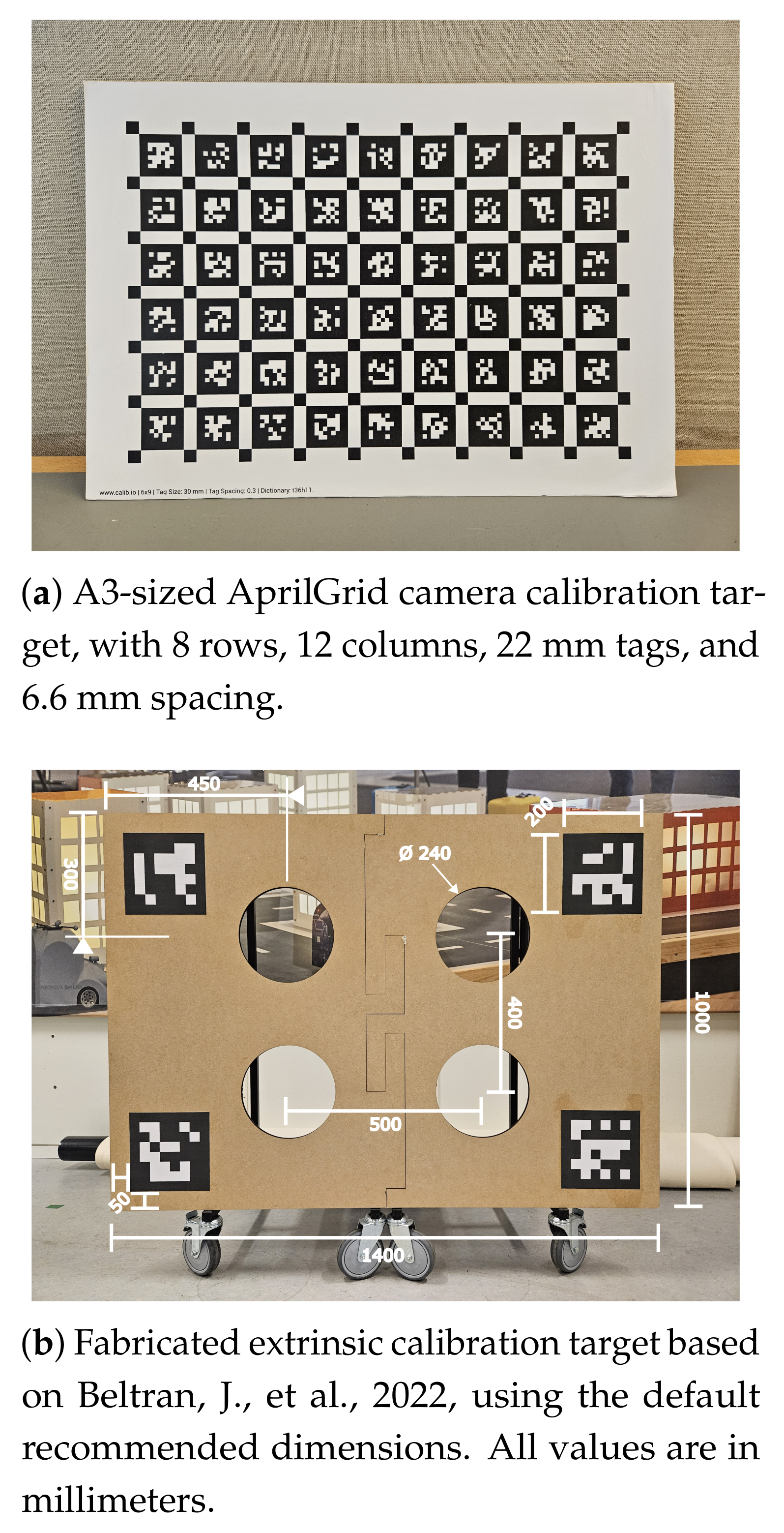
3.4.2. LiDAR–Camera Extrinsic Calibration

To find the relative transformation ${\mathbf{T}}_{l\to c}$ between the LiDAR and camera when sensors are not configured in a predetermined rigid structure, the method described in [56] is utilized. It is a two-stage solution for calibrating between pairs of monocular cameras, stereo cameras, and LiDARs, using a custom calibration pattern featuring four circular holes and four ArUco markers [57]. For this purpose, the calibration target board displayed in Figure 4b was manufactured. Over this, the applied method localizes the centroids of the holes in the target across the two sensors being calibrated and then aligns the two sets of 3D reference points. The following is an overview of the process described in [56]. It should be noted that details on calibrating with stereoscopic cameras are briefly covered solely for the sake of completeness.

Reference Point Estimation

In the first place, the goal is to localize the calibration target and estimate the center points of the holes within, relative to the individual sensors. This is carried out frame-by-frame, per sensor. Here, there are two pathways: one for 3D input and one for monocular input. Stereo-camera feeds are pre-processed into a 3D point cloud and then later used similarly to the LiDAR feed. In both cases, user-adjustable pass-through filters are applied to limit the search space. This requires user intervention, specific to the current physical calibration setup. Edge points are then identified. For LiDARs, depth discontinuities in the point cloud are used to detect edges [58]. This assumes that points resulting from LiDAR rays passing through the calibration target holes exist, so care must be taken to not leave excessive open space behind the target, nor filter these points out in the preceding step. An example of the visualization output of the edge detection procedure is presented in Figure 5a. For stereo cameras, a Sobel filter [59] is applied to one of the two stereo images, and points are mapped to the resulting pixel values. Points with sufficiently low values are discarded. It is at this point that the two modalities are treated similarly. A RANdom Sample Consensus (RANSAC) algorithm [60] is applied to the filtered point cloud data in order to fit a plane model, representing the target plane surface. The edge-points from the previous step are filtered using the obtained plane model, such that the resulting point cloud only contains points belonging to the target.

Next, the remaining points are projected on the planar model, resulting in a 2D point cloud. The circular holes are then extracted using a 2D circle segmentation. This is performed iteratively, removing inliers, until the remaining points are insufficient to describe further circles. At least four circles must be found to proceed, otherwise the current frame is discarded. Monocular cameras rely on using the four ArUco markers as an ArUco board [57] to estimate the relative position of the target. Examples of successfully captured camera projections are displayed in Figure 5b. Once circle centers have been found, the processing of sensor data across modalities are the same. To rule out incorrect detections, a geometric consistency check is performed. The circle center points are grouped in sets of four, and the dimensions of the rectangle they form together are compared against what is theoretically expected. The assumption is that there should only be one valid, geometrically consistent set. If more than one, or zero, valid sets are found, the frame is discarded. Otherwise, the center-points are converted back into 3D space, and the resulting cloud of four points is considered to be valid reference points. Having a single set of reference points per sensor is technically sufficient, but to reduce potential errors, such as from sensor noise, multiple sets are accumulated per sensor, i.e., 30, and verified using Euclidean clustering [61]. In the case of detecting more than the expected four clusters, the data are considered unreliable, or else cluster centroids are used as reference points for the second stage. Furthermore, Ref. [56] allows for (and recommends) accumulating reference points over P target poses as to generate $4\times P$ reference points, adding further constraints in order to improve the final results.

Registration Procedure

In the second place, the goal is to find the rigid transformation that best aligns the reference point sets with each other. This is handled as a multi-objective optimization, involving $4\times P$ objective functions. First, the reference points must be paired so that each reference point from one sensor is associated with the corresponding reference point from the other sensor. There is no guarantee that reference points in each set are in the same order, so to ensure correct association, the four reference points per target are converted to polar coordinates, and the top-most point (i.e., lowest inclination) is identified. From hereon, the remaining points can then be identified by comparing distances to them and thus paired correctly.

3.5. Image-Based Corrosion Identification

In this work, we rely on the popular Deep Neural Network architecture, U-Net [53], for image-based semantic segmentation. U-Net derives from the fully convolutional network introduced in [62], with modifications tailored to facilitate training with small image samples while surpassing its predecessor in accuracy. The architecture of U-Net comprises a conventional convolutional network, coupled with two pathways. The contracting path initiates with two 3 × 3 unpadded convolutions, succeeded by rectified linear units (ReLUs) and downsampling through 2 × 2 max pooling operations. In the expansive path, the feature map undergoes upsampling through 2 × 2 convolutions, followed by cropping to address the loss of border pixels during convolutions. Subsequently, the cropped feature map from the contracting path is concatenated, and 3 × 3 convolutions are applied, followed by rectified linear units (ReLUs) as illustrated in Figure 6. The use of convolutional layers by U-Net with small receptive fields promotes the extraction of intricate hierarchical features, contributing to its robust representation learning capabilities. The adaptability of the architecture to limited training data sets it apart, making it suitable for applications where obtaining extensive labeled samples poses challenges. The symmetric structure of U-Net, with its balanced encoding and decoding paths, plays a pivotal role in maintaining spatial relationships, enhancing feature retention, and boosting its overall performance. A clever combination of skip connections, convolutional layers and adaptability to varied data sizes allows achieving high accuracy with limited training data.

3.6. LiDAR-Based Localization and Mapping

Our proposed pipeline for mapping and localization combines two methods. The first, offline, employs a graph-based SLAM approach to build a reference point cloud map of the environment. The second, online, employs a unscented Kalman filter (UKF) [63]-based approach on top of the reference map to estimate in real time the location of the sensor apparatus.

3.6.1. Graph-Based LiDAR SLAM

LiDAR-based Graph-SLAM is a sensor fusion technique that utilizes a graph structure to represent the relationships between different poses (positions and orientations) of a LiDAR system over time, along with the associated LiDAR measurements. The optimization process seeks to simultaneously estimate the robot’s trajectory and create a consistent map of the environment. A graph $G=(V,E)$ is built over time, where V is the set of vertices representing sensor poses, and E is the set of edges representing constraints between these poses. The optimal node configuration in the graph is found using non-linear optimization techniques to minimize the error introduced by the constraints. Let ${\mathbf{p}}_t$ be the sensor poses at t and ${\mathbf{r}}_{t,t+1}$ be the relative sensor poses between t and $t+1$ estimated via scan matching [64]. We add them to the pose graph as nodes $\left[{\mathbf{p}}_0,...,{\mathbf{p}}_N\right]$ and edges $\left[{\mathbf{r}}_{0,1},...,{\mathbf{r}}_{N-1,N}\right]$. The graph is optimized using the g2o [65] framework to build a globally consistent 3D map of the environment. To compensate for accumulated pose errors during mapping, the approach allows incorporating ground plane constraints in the graph pose optimization. The final output of the algorithm is a map $\mathbb{M}$ of size M, comprising a finite set of points in ${\mathbb{R}}^3$. Let us denote by ${\mathbf{m}}_i\in \mathbb{M},i\in \{1,...,M\}$, each point belonging to $\mathbb{M}$.

3.6.2. Real-Time LiDAR-Based Localization

During the online localization phase, the localization system [32] estimates its own pose on the previously created 3D point cloud map by combining a scan-matching algorithm with an angular velocity-based pose predictor. A UKF [63] is used for sequential Bayesian estimation of the pose of the LiDAR–camera sensor apparatus. The scan matching utilizes a Normal Distribution Transform (NDT) [64] for estimating the LiDAR motion between consecutive frames, which outperforms other scan matching approaches, such as the iterative closest point (ICP) [66].

3.7. Semantic–Geometric Mapping

In order to fuse semantic information with the 3D map of the environment, we utilize the known camera intrinsics, extrinsics between the LiDAR and the camera, and the pose between the LiDAR and the map, given by the localization system. Given an image $\mathcal{I}$ provided by the system’s semantic segmentation algorithm, the semantic color information is projected into the map by combining the transformation between the map and the LiDAR, computed by the localization system ${\mathbf{T}}_{\mathbf{m}\to \mathbf{l}}$, the transformation between the LiDAR and the camera optical center ${\mathbf{T}}_{\mathbf{l}\to \mathbf{c}}$. More specifically, for each point belonging to the map, we compute the corresponding image pixel, using homogeneous coordinates according to

$${\mathbf{u}}_i=\mathbf{K}{\mathbf{T}}_{l\to c}{\mathbf{T}}_{c\to m}{\mathbf{m}}_i\mathrm{with}{\mathbf{u}}_i=\left[\begin{array}{c}u\\ v\\ 1\end{array}\right],{\mathbf{m}}_i=\left[\begin{array}{c}{x}_m\\ y_m\\ z_m\\ 1\end{array}\right]$$

(7)

and if the point falls within the image plane, its corresponding color is updated, by averaging its current RGB values with the corresponding image pixel one.

4. Experimental Validation and Performance Evaluation

In this Section, we provide relevant considerations about the hardware sensor apparatus; and we describe the indoor and outdoor test environments selected for validation and assessment of the performance of the proposed system in realistic conditions.

4.1. Hardware Design and Sensor Selection

As briefly described in Section 3.2, the design of the portable sensor holder was a critical aspect behind the efficient data collection in various applications, such as environmental monitoring or industrial inspections. The designed sensor holder is versatile, providing a stable platform for mounting sensors of different sizes and types. In our implementation, we utilized an Ouster OS1 32 Rev 06 LiDAR and a RealSense d435i camera. The design was selected to offer ease of mobility to capture diverse environments and facilitate data acquisition. We selected 3D-printed material, to ensure easy adaptations during prototyping (e.g., the change of sensors) and ensure durability in challenging conditions while being lightweight for comfortable use. An ergonomic design that prioritizes user comfort and ease of handling is crucial for prolonged data collection tasks. Additionally, the sensor holder incorporates features such as screw holes to facilitate the deployment and interchange of sensors.

Complementing the sensor holder, the design of a backpack for data collection plays a pivotal role in ensuring seamless mobility and accessibility of necessary equipment. The backpack was engineered to be lightweight and easy to carry for long periods of time, distributing the weight evenly and reducing strain on the user during extended periods of data collection. Compartments within the backpack should be strategically arranged to accommodate the sensor holder, ensuring secure storage and easy access. Integration of a power supply system for sensors, along with cable management solutions, is vital to sustain prolonged data collection sessions. The backpack design prioritizes user comfort with padded shoulder straps and a ventilated back panel, thus mitigating discomfort caused by extended wear. Furthermore, the incorporation of smart features such as ground truth markers from reference external positioning systems in given environments allows for flexibility and easy system integration, making the backpack an integral component of a well-rounded field data collection system. A picture of the complete hardware setup including both the sensor holder and the backpack is shown in Figure 2c.

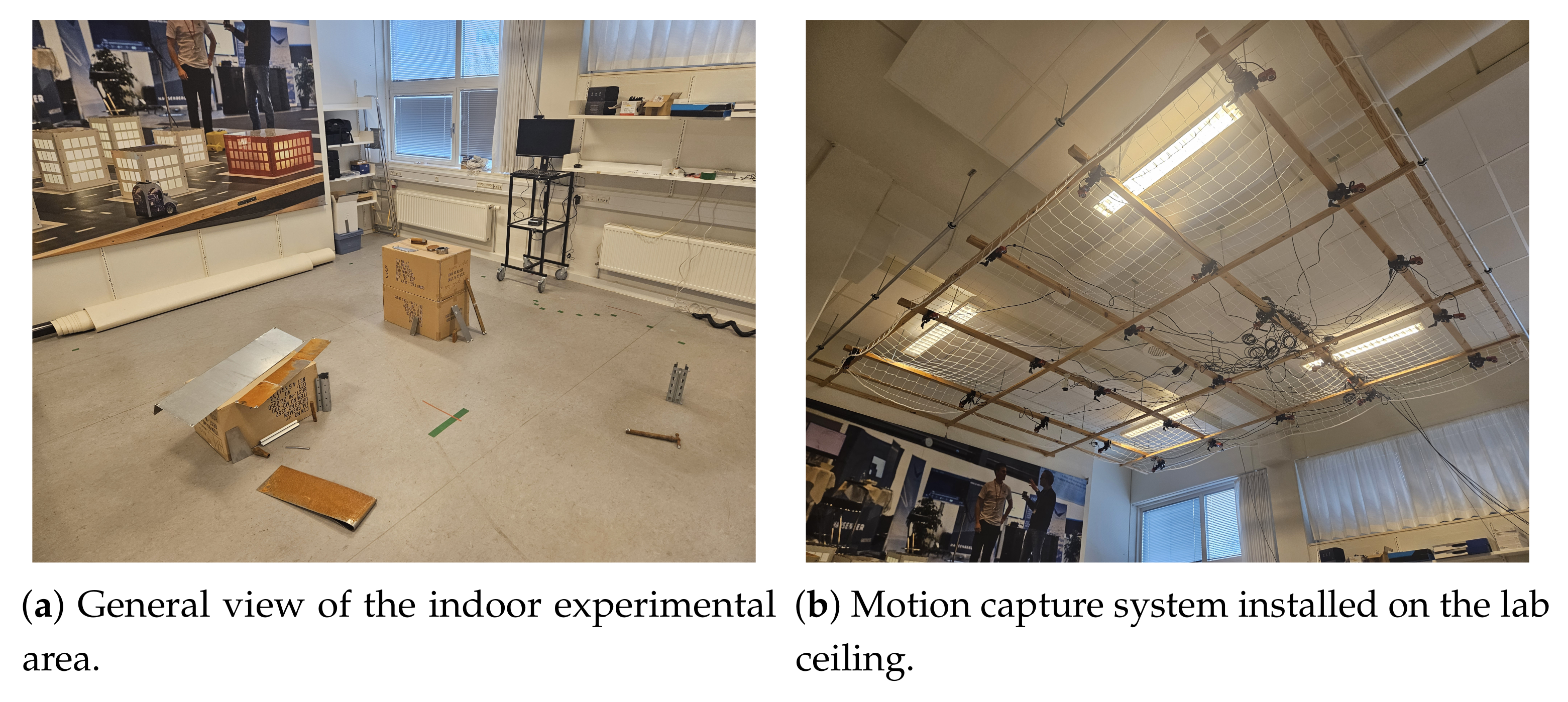
4.2. Indoor Laboratory Experimentation

In order to test the proposed system and compare our solutions for LiDAR-based localization, experimental data recording sessions in an indoor laboratory setting were conducted. The purpose for these recordings was to create datasets for assessing the performance of the localization algorithms, using a motion capture system. Furthermore, uncorroded and corroded metal parts were placed in the environment to allow testing the performance of the corrosion detection algorithms. An image of the environment containing metal parts is displayed in Figure 7a. The experimental area was a 5 × 5 m open space surrounded by storage areas with metallic shields, walls with metallic shelves and electronic equipment, metal-coated windows, and radiators, and also workplaces for electronic prototype assembly. Above the test area, an Optitrack motion capture system, based on infrared technology was installed as a calibrated reference system. This is shown in Figure 7b. The experimentation considered the integrated system with the operational sensor holder and the backpack support, which was further equipped with a rigid-body tracking marker on top of the LiDAR in order to be detected by the reference Optitrack system.

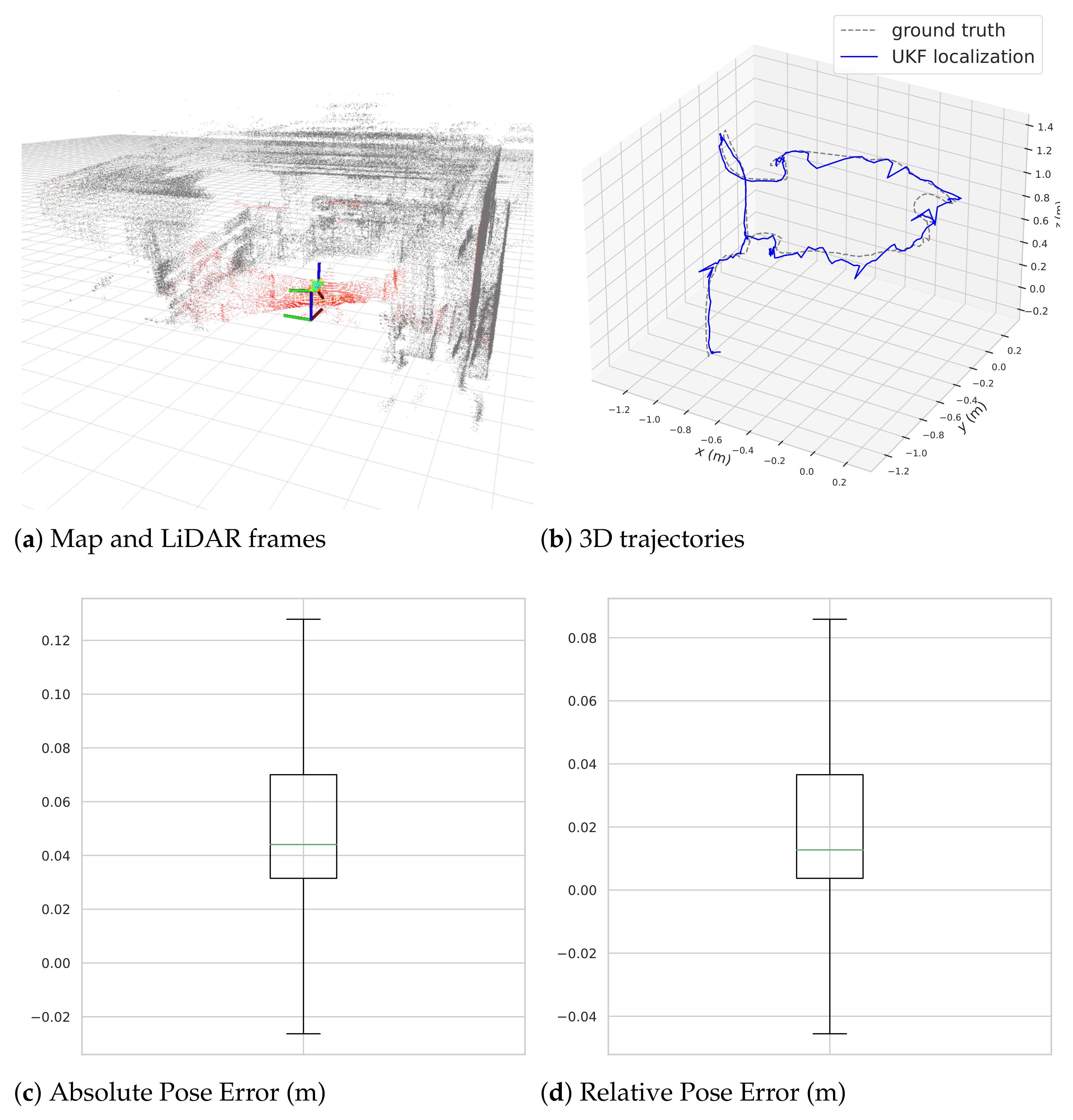
4.2.1. Localization and Mapping Performance

In order to assess the performance of the indoor localization and mapping algorithms, we designed a trajectory evaluation procedure, simultaneously logging and processing spatial information with our integrated system and tracking the absolute calibrated position with the reference motion capture system, whose ground truth acquisition exhibits a precision in the order or 0.1 mm [67]. To quantitatively evaluate the performance of the algorithms, we compared the trajectory given by the Optitrack ground truth system with the one computed by the UKF localization algorithms implemented in our automated system. More specifically, trajectories were temporally and spatially aligned using the Umeyama alignment algorithm [68], and the absolute pose error (APE) and relative pose error (RPE) were used for the evaluation, assessing the consistency and accuracy of the trajectory of the measurement device.

While the absolute pose error (APE) focuses on the accuracy of the overall position and orientation of the LiDAR–camera system in the ground truth frame, i.e., global trajectory consistency, the relative pose error (RPE) is concerned with the accuracy of the changes in pose between consecutive measurements in a local coordinate frame, hence suitable for measuring drift in odometry systems. While the APE focuses on the accuracy of the overall position and orientation of the LiDAR–camera system in the ground truth frame, i.e., global trajectory consistency,

$${\mathrm{APE}}_i=∥P_i^{\mathrm{est}}-P_i^{\mathrm{gt}}∥$$

(8)

where $P_i^{\mathrm{est}}$$P_i^{\mathrm{gt}}$ are the system estimated pose and the Optitrack ground truth pose at the i-th instant, respectively, the RPE is concerned with the accuracy of the changes in pose between consecutive measurements at instants i and $i+\Delta$: $(P_i^{\mathrm{est}},P_i^{\mathrm{gt}}),$ and $(P_{i+\Delta }^{\mathrm{est}},P_{i+\Delta }^{\mathrm{gt}})$, hence being suitable as a drift measurement in odometry systems,

$${\mathrm{RPE}}_{i+\Delta }=∥{\left(P_i^{\mathrm{est}}\right)}^{-1}·P_{i+\Delta }^{\mathrm{est}}-{\left(P_i^{\mathrm{gt}}\right)}^{-1}·P_{i+\Delta }^{\mathrm{gt}}∥$$

(9)

Figure 8 summarizes the main results achieved in the localization and mapping test. Figure 8a depicts the map point cloud obtained with the SLAM algorithm and the map and LiDAR reference frames during online localization. This figure can be compared to the picture in Figure 7a. As illustrated, the dynamic range of our LiDAR suffices to achieve a detailed and realistic description of the surroundings, trespassing metallic surfaces and walls up to a distance of approximately 10 m. Figure 8b–d show the 3D trajectories estimated by the ground truth system and by the UKF localization algorithm of our automated device, as well as the absolute and relative pose errors, respectively. It is observable in the comparison between trajectories in Figure 8b that the one estimated by our UKF algorithm presents slightly larger variability than the one achieved over the reference system. In absolute terms, both are very close and comparable, but the one by the Optitrack system is smoother. The APE and RPE results in Figure 8c,d demonstrate the high accuracy of the implemented LiDAR-based localization system. Our system achieved a median positioning accuracy of $0.05$ m and $0.01$ m in terms of APE and RPE. In terms of variability, the APE presents a standard deviation of approximately $\pm 0.02$ m and maximum variations of $\pm 0.08$ m. For the RPE, the standard deviation is also approximately $\pm 0.02$ m, and the maximum variation is $\pm 0.06$ m. One setback, though, of the employed method resides on the fact that it needs a good pose initialization. However, this limitation can be easily surpassed with the use of Monte Carlo Localization (MCL) based methods (e.g., [69]), at the cost of increased computation effort.

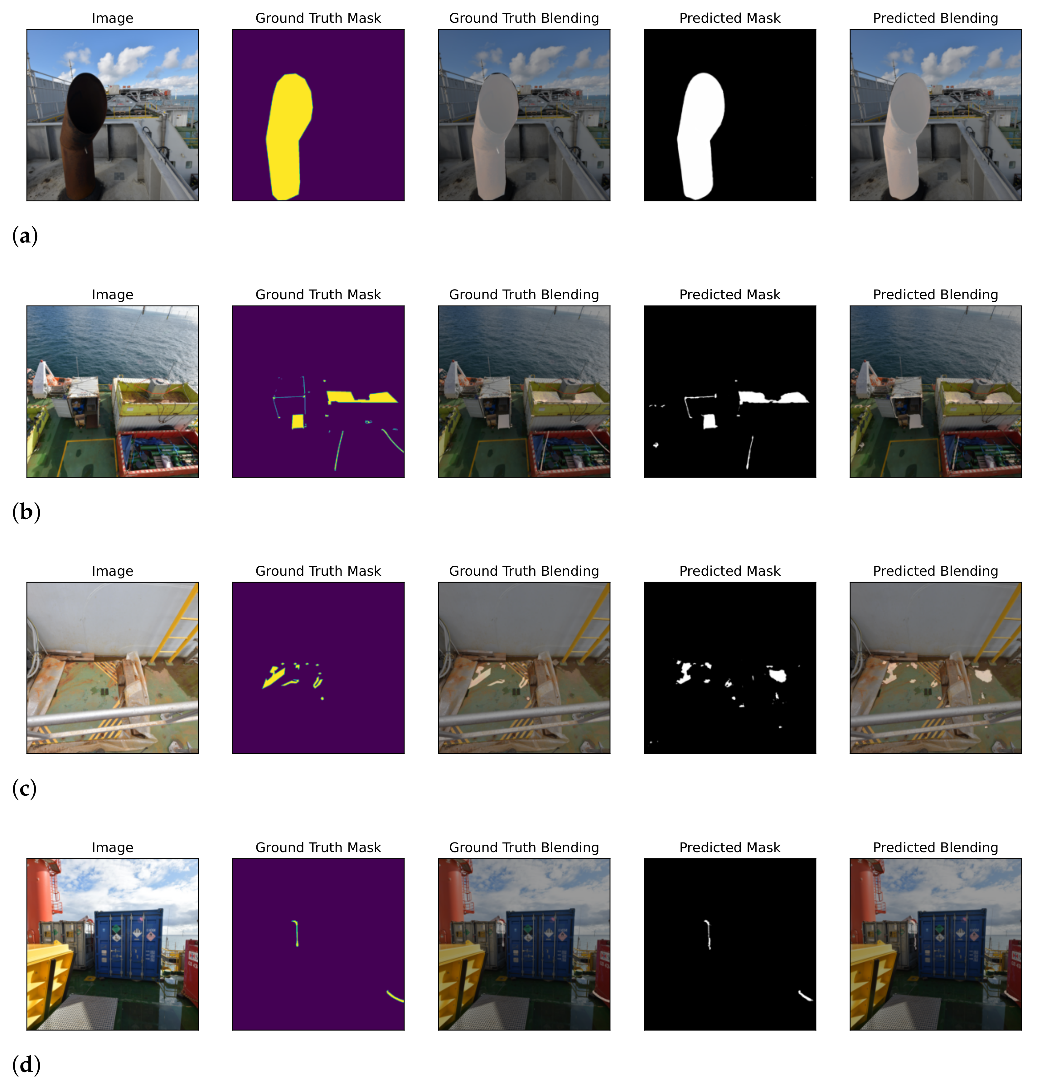
4.3. Semantic Segmentation in Outdoor Offshore Conditions

In this section, we conduct a comparative analysis of advanced semantic segmentation networks outlined in the preceding section, specifically focusing on their effectiveness in segmenting corrosion in metallic structures. Throughout our experiments, we employed a 12th Gen Intel® Core™ i9-12900KF processor (24 cores) and a GeForce RTX 3090ti graphics card for both training and testing. The dataset utilized for training and testing comprises a total of $14,265$ labeled images that were captured in a realistic high-definition outdoor offshore environment using a DSLR camera and were manually annotated using an online labeling tool [70]. The dataset includes images of metal surfaces exhibiting various corrosion types, namely, uniform corrosion, galvanic corrosion, and pitting corrosion. These corrosion types were selected due to their prevalence and visual distinctiveness in industrial contexts. The metal surfaces in the dataset include steel, aluminum, and copper, covering a range of typical industrial materials.

4.3.1. Evaluation Metrics

Evaluating the performance of semantic segmentation tasks requires simultaneously evaluating pixel-level classification and localization accuracy. Let us consider the number of true positive ($TP$), false positive ($FP$), true negative ($TN$), and false negative ($FN$) predictions. The following metrics are defined to evaluate the performance of our semantic segmentation model: Intersection over Union (IoU), Dice Similarity Coefficient (or F-score), Precision, and Recall.

$IoU$ measures the amount of overlap between ground truth and prediction masks, according to

$$IoU={\displaystyle \frac{TP}{TP+FN+FP}}$$

(10)

The F-score is a widely used metric in CV for evaluating the similarity between two images. It penalizes both under-segmentation and over-segmentation. The metric is calculated using the following formula:

$$F_1={\displaystyle \frac{2TP}{2TP+FP+FN}}$$

(11)

Precision measures how accurate the model is at finding true positives, i.e., from all pixels that the model estimates as belonging to the segmentation mask, how many are correctly estimated according to the ground truth. Precision is computed according to the following expression:

$$Precision={\displaystyle \frac{TP}{TP+FP}}$$

(12)

Recall measures the true-positive rate, i.e., from the pixels belonging to ground truth masks, how many are predicted. Recall is computed according to the following expression:

$$Recall={\displaystyle \frac{TP}{TP+FN}}$$

(13)

Considering that the ground truth has missing annotations, predictions may be incorrectly classified as being false positive. Therefore, recall is more relevant than precision when ground truth masks are incomplete.

4.3.2. Quantitative and Qualitative Analysis

In our experimental approach, we trained a U-Net semantic segmentation model, using random crops of size $1024\times 1024$ extracted from the our dataset collected in an offshore windmill substation, comprising 14,265 images, of resolution $3840\times 2160$ (i.e., 4K). The training batch size was set to 8 and the number of training epochs to 80. The dataset was partitioned into training, validation, and testing. As a reference,

Table 1. Dataset used for training and validating the semantic segmentation networks.

Total Images in Dataset
training	8559 (80%)
validation	2853 (10%)
testing	2853 (10%)

summarizes the sample sizes of each subset. To address the challenge of limited training data, we leveraged transfer learning by pre-training the model on the large-scale ImageNet dataset [71]. This allowed the network to start with rich, general-purpose visual features, which significantly improves performance when fine-tuning on smaller, domain-specific datasets. Specifically, we used a ResNet-34 backbone in our U-Net architecture [72], which offers a strong trade-off between depth and efficiency, making it well suited for capturing both low-level textures and high-level structural patterns in corrosion images.In addition, we applied data augmentation techniques (e.g., random rotations, flips, and color jittering) to synthetically expand the dataset and improve generalization. These steps help reduce overfitting and make the model more robust to variations in surface appearance and lighting, thus achieving high accuracy even with limited annotated samples.The model underwent pre-training on the ImageNet [71] dataset. We use a ResNet-34 as our U-Net backbone [72], which consists of 34 layers, being popular in image recognition tasks, due to its clever balance between depth and computational efficiency.

Figure 9 depicts the training and validation evolution curves for the Dice loss, computed from Equation (11), and IoU metrics, computed from Equation (10), for 80 training epochs. As shown, the IoU score improves steeply until epochs 40–50, saturating around $0.9$ and $0.5$, for the training and validation curves, respectively. Figure 10 shows, qualitatively, the performance of U-Net on different scenes. U-Net is capable of identifying most ground truth spots while correctly identifying corrosion spots missed by the labeler. Given the difficulty of accurately labeling corrosion, especially when small spots are easily overlooked by human annotators, precision, defined as in Equation (12), may not be the most suitable metric for evaluating task effectiveness in this context. As quantitatively shown in

Table 2. U-Net performance results on corrosion segmentation in offshore environments.

Model	IoU Score	Precision	Recall	F-Score	Avg. Inference Time
UNET-resnet34 585256922	0.5852	0.7368	0.7065	0.6922	0.0445 s

, the method exhibits fast average inference times ($0.0445$ s), being suitable for real-time application. Although our model achieves high precision when compared with similar corrosion identification approaches, e.g., [73], being able to recognize most ground truth corrosion pixels, without many false positives, recall is relatively low, due to a high rate of false negatives, i.e., missed corrosion spots in the ground truth. We hypothesize that this is due to a relatively high number of missed corrosion spots by the labeler. Although a detailed comparative evaluation with varying training sizes is beyond the scope of this work, we refer the interested reader to our previous study dedicated to corrosion segmentation [41], where we thoroughly evaluated multiple state-of-the-art models on the same dataset under different training conditions.

4.4. Operational Validation in an Industrial Manufacturing Scenario

In order to further validate our automated corrosion detection system in operational industrial settings, a test was performed at the Aalborg University Smart Production Lab. This realistic manufacturing environment is composed of a small industrial research factory lab devoted to various areas devoted to robotic automation, production technologies, palletizing, storage, welding, etc. We conducted data recordings traversing a large part of the asset both inside and outside the main factory building, testing and validating the LiDAR and camera data recordings in both indoor and outdoor settings. In relation to this validation test campaign, Figure 11 illustrates both a human operator handling the measurement device and backpack and example pictures of the indoor industrial environment captured by the camera.

Performance levels during the outdoor tests are assumed to be the same as the indoor, reported in Section 4.2.1 and Section 4.3.2 for both positioning accuracy and precision and semantic segmentation accuracy. Our LiDAR-based proposed system should be capable of positioning the device within the environment with similar accuracy in indoor and outdoor settings. However, we provide only qualitative measures in this setting since a ground truth system was not available for outdoors. It should be noted that, due to LiDAR hardware operational limitations, the system may struggle in large outdoor open spaces, where nearest obstacles are far and cannot be properly detected by the sensor. However, this is not expected to be an important limitation given the main purpose of the system, which is detecting corrosion. This typically implies measuring in short distances to the targeted surfaces. Furthermore, the dataset includes scenes with natural lighting variations such as shadows, direct sunlight, and diffuse illumination captured at different times of day. These variations introduce meaningful environmental complexity to the segmentation task. However, due to logistical constraints during data collection, it was not possible to record sequences under a broader range of conditions such as nighttime, overcast weather, or adverse environmental settings. We acknowledge this as a limitation of the current work and plan to address it in future dataset extensions to support more comprehensive benchmarking across diverse environmental scenarios. Figure 12 shows the maps created offline with the proposed pipeline, with one of the data recording sequences. The results demonstrate the applicability of the proposed system in relevant scenarios, even in outdoor conditions, for creating accurate multi-modal (RGB and semantic) 3D maps. However, during this test, we empirically found that the semantic segmentation approach is noisy and error-prone in the presence of small drifts in the localization system. This setback can be overcome by using a probabilistic approach for fusing semantic and point cloud data that accounts both for calibration and semantic estimation errors.

5. Conclusions and Future Work

In this work, we presented the design and implementation of a complete automated system for corrosion identification and 3D mapping in industrial environments. The proposed system comprises a portable sensor holder for a 3D LiDAR and an RGB camera as well as a backpack for computing support. The system leverages the accuracy of LiDAR data for 3D localization and mapping, with RGB camera information for semantic segmentation of corroded metal structures. Our proposed framework allows building a 3D geometric–semantic map by fusing semantic data with a prior known 3D map, via known camera and LiDAR calibration parameters, and a real-time UKF LiDAR-based localization system.

A set of indoor experiments assessed the performance of the individual parts of the mapping and localization system in a laboratory environment by calibration against a reference infrared-based motion capture system, achieving an accuracy better than $0.02$ m and $0.05$ m in terms of average absolute and relative pose error. The accuracy of the semantic segmentation algorithms was also evaluated. This was performed based on available outdoor offshore datasets. To provide a meaningful comparison within time constraints, we focused on evaluating our LiDAR-based mapping methods only, which currently represent the strongest baseline for structural mapping. We further extended these methods by incorporating color information, enabling them to detect and map corrosion spots in addition to geometry. This fusion allowed for a more direct comparison with our image-based approach in terms of both spatial accuracy and corrosion localization. Although comparisons against other solutions based on costly and specialized equipment was not possible, we demonstrated the robustness and high accuracy of state-of-the-art computer vision recognition ($0.69$ F-score in semantic segmentation) and state estimation ($0.045$ m in 3D localization accuracy) methods—which have been successfully applied in other domains (e.g., robotics and biomedical imaging)—for mapping defects (e.g., corrosion) in metal structures and offshore or industrial assets. Further, a validation campaign was performed in an industrial scenario, validating the reported performance and accuracies of the positioning and corrosion detection mechanism for both indoor and outdoor environments.

For future work, we intend to replace the current UKF-based localization system with a Monte Carlo one [74] to avoid the need of knowing, in advance, the approximate initial location of the system. Also, we intend to improve our semantic map representation, with one that allows fusing semantic and geometric data over time in a probabilistic fashion (e.g., using a probabilistic semantic occupancy grid [75]). Ultimately, we plan to enhance our existing semantic segmentation algorithm by training with large amounts of synthetically generated data.

While the system shows strong performance in controlled tests, practical deployment in industrial settings presents challenges—particularly with false positives. These occur when non-corroded areas (e.g., stains, shadows, or manufacturing marks) are mistakenly flagged as corrosion. Such errors can lead to unnecessary inspections or maintenance actions, increasing operational costs and reducing trust in the system over time.

False positives also raise the risk of alarm fatigue, where frequent inaccurate alerts may desensitize technicians or lead to ignored warnings. This is especially critical in automated inspection workflows, where system reliability directly affects operational efficiency. Improving precision, incorporating confidence thresholds, or adding a human-in-the-loop validation step may help mitigate these issues and enhance the system’s practical reliability. Finally, the current hardware setup would also benefit from several improvements, namely, more accurate sensors; gimbal-based sensor stabilization; user-experience-related design enhancements, such as a permanent fixture for the keyboard and the display; improved onboard computational devices and batteries. The overall design should be optimized taking also into account the apparatus physical weight and the data-gathering requirements (e.g., runtime).

References

1. Koch, G.H.; Brongers, M.P.H.; Thompson, N.G.; Virmani, Y.P.; Payer, J.H.; CC Technologies, Inc. NACE International. Corrosion Cost and Preventive Strategies in the United States [Final Report]; Technical Report FHWA-RD-01-156, R315-01. Federal Highway Administration: Washington, DC, USA, 2002. [Google Scholar]
2. Koch, G. 1—Cost of Corrosion. In Trends in Oil and Gas Corrosion Research and Technologies; El-Sherik, A.M., Ed.; Woodhead Publishing Series in Energy; Woodhead Publishing: Boston, MA, USA, 2017; pp. 3–30. [Google Scholar] [CrossRef]
3. Revie, R.W. Corrosion and Corrosion Control: An Introduction to Corrosion Science and Engineering, 4th ed.; John Wiley & Sons: Hoboken, NJ, USA, 2008. [Google Scholar] [CrossRef]
4. Liu, Y.; Hajj, M.; Bao, Y. Review of Robot-Based Damage Assessment for Offshore Wind Turbines. Renew. Sustain. Energy Rev. 2022, 158, 112187. [Google Scholar] [CrossRef]
5. Schjørring, A.; Cretu-Sircu, A.L.; Rodriguez, I.; Cederholm, P.; Berardinelli, G.; Mogensen, P. Performance Evaluation of a UWB Positioning System Applied to Static and Mobile Use Cases in Industrial Scenarios. Electronics 2022, 11, 3294. [Google Scholar] [CrossRef]
6. Crețu-Sîrcu, A.L.; Schiøler, H.; Cederholm, J.P.; Sîrcu, I.; Schjørring, A.; Larrad, I.R.; Berardinelli, G.; Madsen, O. Evaluation and Comparison of Ultrasonic and UWB Technology for Indoor Localization in an Industrial Environment. Sensors 2022, 22, 2927. [Google Scholar] [CrossRef]
7. Nastac, D.I.; Lehan, E.S.; Iftimie, F.A.; Arsene, O.; Cramariuc, B. Automatic Data Acquisition with Robots for Indoor Fingerprinting. In Proceedings of the 2018 International Conference on Communications (COMM), Bucharest, Romania, 14–16 June 2018; pp. 321–326. [Google Scholar] [CrossRef]
8. Fatihah, S.N.; Dewa, G.R.R.; Park, C.; Sohn, I. Self-Optimizing Bluetooth Low Energy Networks for Industrial IoT Applications. IEEE Commun. Lett. 2023, 27, 386–390. [Google Scholar] [CrossRef]
9. Wang, F.; Yu, Y.; Yang, D.; Wang, L.; Xing, J. First Potential Demonstrations and Assessments of Monitoring Offshore Oil Rigs States Using GNSS Technologies. IEEE Trans. Instrum. Meas. 2022, 71, 1–15. [Google Scholar] [CrossRef]
10. Specht, C.; Pawelski, J.; Smolarek, L.; Specht, M.; Dabrowski, P. Assessment of the Positioning Accuracy of DGPS and EGNOS Systems in the Bay of Gdansk using Maritime Dynamic Measurements. J. Navig. 2019, 72, 575–587. [Google Scholar] [CrossRef]
11. Angelats, E.; Espín-López, P.F.; Navarro, J.A.; Parés, M.E. Performance Analysis of The IOPES Seamless Indoor–Outdoor Positioning Approach. Int. Arch. Photogramm. Remote. Sens. Spat. Inf. Sci. 2021, XLIII-B4-2021, 229–235. [Google Scholar] [CrossRef]
12. Liu, L.; Tan, E.; Cai, Z.Q.; Zhen, Y.; Yin, X.J. An Integrated Coating Inspection System for Marine and Offshore Corrosion Management. In Proceedings of the 2018 15th International Conference on Control, Automation, Robotics and Vision (ICARCV), Singapore, 18–21 November 2018; pp. 1531–1536. [Google Scholar] [CrossRef]
13. Ricardo Luhm Silva, O.C.J.; Rudek, M. A road map for planning-deploying machine vision artifacts in the context of industry 4.0. J. Ind. Prod. Eng. 2022, 39, 167–180. [Google Scholar] [CrossRef]
14. Choi, J.; Son, M.G.; Lee, Y.Y.; Lee, K.H.; Park, J.P.; Yeo, C.H.; Park, J.; Choi, S.; Kim, W.D.; Kang, T.W.; et al. Position-based augmented reality platform for aiding construction and inspection of offshore plants. Vis. Comput. 2020, 36, 2039–2049. [Google Scholar] [CrossRef]
15. Irmisch, P.; Baumbach, D.; Ernst, I. Robust Visual-Inertial Odometry in Dynamic Environments Using Semantic Segmentation for Feature Selection. ISPRS Ann. Photogramm. Remote Sens. Spat. Inf. Sci. 2020, V-2-2020, 435–442. [Google Scholar] [CrossRef]
16. Wen, F.; Pray, J.; McSweeney, K.; Hai, G. Emerging Inspection Technologies-Enabling Remote Surveys/Inspections. In Proceedings of the OTC Offshore Technology Conference, Huston, TX, USA, 6–9 May 2019. [Google Scholar] [CrossRef]
17. Roberge, P.R. Corrosion Inspection and Monitoring, 1st ed.; Wiley Series in Corrosion; John Wiley & Sons: Hoboken, NJ, USA, 2007. [Google Scholar]
18. Kapoor, K.; Krishna, K.S.; Bakshu, S.A. On Parameters Affecting the Sensitivity of Ultrasonic Testing of Tubes: Experimental and Simulation. J. Nondestruct. Eval. 2016, 35, 56. [Google Scholar] [CrossRef]
19. Sophian, A.; Tian, G.; Fan, M. Pulsed Eddy Current Non-destructive Testing and Evaluation: A Review. Chin. J. Mech. Eng. 2017, 30, 500–514. [Google Scholar] [CrossRef]
20. Bortak, T.N. Guide to Protective Coatings Inspection and Maintenance; US Department of the Interior, Bureau of Reclamation: Washington, DC, USA, 2002; p. 118. [Google Scholar]
21. Kelly, R.G.; Scully, J.R.; Shoesmith, D.; Buchheit, R.G. Electrochemical Techniques in Corrosion Science and Engineering; CRC Press: Boca Raton, FL, USA, 2002. [Google Scholar] [CrossRef]
22. Doshvarpassand, S.; Wu, C.; Wang, X. An overview of corrosion defect characterization using active infrared thermography. Infrared Phys. Technol. 2019, 96, 366–389. [Google Scholar] [CrossRef]
23. Choi, K.Y.; Kim, S. Morphological analysis and classification of types of surface corrosion damage by digital image processing. Corros. Sci. 2005, 47, 1–15. [Google Scholar] [CrossRef]
24. Lovejoy, D. Magnetic Particle Inspection: A Practical Guide, 1st ed.; Springer Netherlands: Dordrecht, The Netherlands, 1993. [Google Scholar] [CrossRef]
25. Zaki, A.; Chai, H.K.; Aggelis, D.G.; Alver, N. Non-Destructive Evaluation for Corrosion Monitoring in Concrete: A Review and Capability of Acoustic Emission Technique. Sensors 2015, 15, 19069. [Google Scholar] [CrossRef]
26. Aharinejad, S.H.; Lametschwandtner, A. Microvascular Corrosion Casting in Scanning Electron Microscopy: Techniques and Applications; Springer Science & Business Media: Vienna, Austria, 1992. [Google Scholar] [CrossRef]
27. Debeunne, C.; Vivet, D. A review of visual-LiDAR fusion based simultaneous localization and mapping. Sensors 2020, 20, 2068. [Google Scholar] [CrossRef]
28. Zhang, Z. A flexible new technique for camera calibration. IEEE Trans. Pattern Anal. Mach. Intell. 2000, 22, 1330–1334. [Google Scholar] [CrossRef]
29. Rehder, J.; Nikolic, J.; Schneider, T.; Hinzmann, T.; Siegwart, R. Extending kalibr: Calibrating the extrinsics of multiple IMUs and of individual axes. In Proceedings of the 2016 IEEE International Conference on Robotics and Automation (ICRA), Stockholm, Sweden, 16–21 May 2016; pp. 4304–4311. [Google Scholar] [CrossRef]
30. Mirzaei, F.M.; Kottas, D.G.; Roumeliotis, S.I. 3D LIDAR–Camera Intrinsic and Extrinsic Calibration: Identifiability and Analytical Least-Squares-Based Initialization. Int. J. Robot. Res. 2012, 31, 452–467. [Google Scholar] [CrossRef]
31. Arshad, S.; Kim, G.W. Role of deep learning in loop closure detection for visual and lidar slam: A survey. Sensors 2021, 21, 1243. [Google Scholar] [CrossRef]
32. Koide, K.; Miura, J.; Menegatti, E. A portable three-dimensional LIDAR-based system for long-term and wide-area people behavior measurement. Int. J. Adv. Robot. Syst. 2019, 16, 1729881419841532. [Google Scholar] [CrossRef]
33. Thrun, S.; Montemerlo, M. The Graph SLAM Algorithm with Applications to Large-Scale Mapping of Urban Structures—Sebastian Thrun, Michael Montemerlo, 2006. Int. J. Robot. Res. 2006, 25, 403–429. [Google Scholar] [CrossRef]
34. Xu, W.; Zhang, F. FAST-LIO: A Fast, Robust LiDAR-Inertial Odometry Package by Tightly-Coupled Iterated Kalman Filter. IEEE Robot. Autom. Lett. 2021, 6, 3317–3324. [Google Scholar] [CrossRef]
35. Urrea, C.; Agramonte, R. Kalman filter: Historical overview and review of its use in robotics 60 years after its creation. J. Sens. 2021, 2021, 9674015. [Google Scholar] [CrossRef]
36. Xu, W.; Cai, Y.; He, D.; Lin, J.; Zhang, F. FAST-LIO2: Fast Direct LiDAR-Inertial Odometry. IEEE Trans. Robot. 2022, 38, 2053–2073. [Google Scholar] [CrossRef]
37. Akai, N.; Hirayama, T.; Murase, H. 3D Monte Carlo Localization with Efficient Distance Field Representation for Automated Driving in Dynamic Environments. In Proceedings of the 2020 IEEE Intelligent Vehicles Symposium (IV), Las Vegas, NV, USA, 19 October 2020–13 November 2020; pp. 1859–1866. [Google Scholar] [CrossRef]
38. Perez-Grau, F.J.; Caballero, F.; Viguria, A.; Ollero, A. Multi-sensor three-dimensional Monte Carlo localization for long-term aerial robot navigation. Int. J. Adv. Robot. Syst. 2017, 14, 1729881417732757. [Google Scholar] [CrossRef]
39. Vizzo, I.; Guadagnino, T.; Mersch, B.; Wiesmann, L.; Behley, J.; Stachniss, C. KISS-ICP: In Defense of Point-to-Point ICP – Simple, Accurate, and Robust Registration If Done the Right Way. IEEE Robot. Autom. Lett. (RA-L) 2023, 8, 1029–1036. [Google Scholar] [CrossRef]
40. Akai, N. Efficient Solution to 3D-LiDAR-based Monte Carlo Localization with Fusion of Measurement Model Optimization via Importance Sampling. arXiv 2023, arXiv:2303.00216. [Google Scholar] [CrossRef]
41. de Figueiredo, R.P.; Bøgh, S. Vision-Based Corrosion Identification Using Data-Driven Semantic Segmentation Techniques. In Proceedings of the 2023 IEEE International Conference on Imaging Systems and Techniques (IST), Copenhagen, Denmark, 17–19 October 2023; pp. 1–6. [Google Scholar] [CrossRef]
42. Seo, H.; Badiei Khuzani, M.; Vasudevan, V.; Huang, C.; Ren, H.; Xiao, R.; Jia, X.; Xing, L. Machine learning techniques for biomedical image segmentation: An overview of technical aspects and introduction to state-of-art applications. Med. Phys. 2020, 47, e148–e167. [Google Scholar] [CrossRef]
43. Tøttrup, D.; Skovgaard, S.L.; Sejersen, J.l.F.; Pimentel de Figueiredo, R. A Real-Time Method for Time-to-Collision Estimation from Aerial Images. J. Imaging 2022, 8, 62. [Google Scholar] [CrossRef]
44. le Fevre Sejersen, J.; Pimentel De Figueiredo, R.; Kayacan, E. Safe Vessel Navigation Visually Aided by Autonomous Unmanned Aerial Vehicles in Congested Harbors and Waterways. In Proceedings of the 2021 IEEE 17th International Conference on Automation Science and Engineering (CASE), Lyon, France, 23–27 August 2021; pp. 1901–1907. [Google Scholar] [CrossRef]
45. De Figueiredo, R.P.; le Fevre Sejersen, J.; Hansen, J.G.; Brandão, M.; Kayacan, E. Real-Time Volumetric-Semantic Exploration and Mapping: An Uncertainty-Aware Approach. In Proceedings of the 2021 IEEE/RSJ International Conference on Intelligent Robots and Systems (IROS), Prague, Czech Republic, 27 September–1 October 2021; pp. 9064–9070. [Google Scholar] [CrossRef]
46. Pimentel de Figueiredo, R.; le Fevre Sejersen, J.; Hansen, J.; Brandão, M. Integrated design-sense-plan architecture for autonomous geometric-semantic mapping with UAVs. Front. Robot. AI 2023, 9, 911974. [Google Scholar] [CrossRef]
47. Gruosso, M.; Capece, N.; Erra, U. Human Segmentation in Surveillance Video with Deep Learning. Multimed. Tools Appl. 2021, 80, 1175–1199. [Google Scholar] [CrossRef]
48. Tao, H.; Zheng, Y.; Wang, Y.; Qiu, J.; Vladimir, S. Enhanced Feature Extraction YOLO Industrial Small Object Detection Algorithm based on Receptive-Field Attention and Multi-scale Features. Meas. Sci. Technol. 2024, 35, 105023. [Google Scholar] [CrossRef]
49. Lin, T.Y.; Maire, M.; Belongie, S.; Hays, J.; Perona, P.; Ramanan, D.; Dollár, P.; Zitnick, C.L. Microsoft COCO: Common Objects in Context. In Proceedings of the 13th European Conference, Zurich, Switzerland, 6–12 September 2014; pp. 740–755. [Google Scholar] [CrossRef]
50. Cordts, M.; Omran, M.; Ramos, S.; Rehfeld, T.; Enzweiler, M.; Benenson, R.; Franke, U.; Roth, S.; Schiele, B. The Cityscapes Dataset for Semantic Urban Scene Understanding. In Proceedings of the 2016 IEEE Conference on Computer Vision and Pattern Recognition (CVPR), Las Vegas, NV, USA, 27–30 June 2016; pp. 3213–3223. [Google Scholar] [CrossRef]
51. Zheng, S.; Lu, J.; Zhao, H.; Zhu, X.; Luo, Z.; Wang, Y.; Fu, Y.; Feng, J.; Xiang, T.; Torr, P.H.; et al. Rethinking Semantic Segmentation from a Sequence-to-Sequence Perspective with Transformers. In Proceedings of the 2021 IEEE/CVF Conference on Computer Vision and Pattern Recognition (CVPR), Nashville, TN, USA, 20–25 June 2021; pp. 6877–6886. [Google Scholar] [CrossRef]
52. He, K.; Gkioxari, G.; Dollár, P.; Girshick, R. Mask r-cnn. In Proceedings of the 2017 IEEE International Conference on Computer Vision (ICCV), Venice, Italy, 22–29 October 2017; pp. 2961–2969. [Google Scholar] [CrossRef]
53. Ronneberger, O.; Fischer, P.; Brox, T. U-Net: Convolutional Networks for Biomedical Image Segmentation. In Proceedings of the 18th International Conference, Munich, Germany, 5–9 October 2015; pp. 234–241. [Google Scholar] [CrossRef]
54. Furgale, P.; Rehder, J.; Siegwart, R. Unified temporal and spatial calibration for multi-sensor systems. In Proceedings of the 2013 IEEE/RSJ International Conference on Intelligent Robots and Systems, Tokyo, Japan, 3–7 November 2013; pp. 1280–1286. [Google Scholar] [CrossRef]
55. Nocedal, J.; Wright, S.J. Numerical Optimization, 2nd ed.; Springer Series in Operations Research and Financial Engineering; Springer: New York, NY, USA, 2006. [Google Scholar] [CrossRef]
56. Beltran, J.; Guindel, C.; Escalera, A.D.L.; Garcia, F. Automatic Extrinsic Calibration Method for LiDAR and Camera Sensor Setups. IEEE Trans. Intell. Transp. Syst. 2022, 23, 17677–17689. [Google Scholar] [CrossRef]
57. Garrido-Jurado, S.; Muñoz-Salinas, R.; Madrid-Cuevas, F.J.; Marín-Jiménez, M.J. Automatic generation and detection of highly reliable fiducial markers under occlusion. Pattern Recognit. 2014, 47, 2280–2292. [Google Scholar] [CrossRef]
58. Levinson, J.; Thrun, S. Automatic Online Calibration of Cameras and Lasers. In Proceedings of the Robotics: Science and Systems, Berlin, Germany, 24–28 June 2013. [Google Scholar] [CrossRef]
59. Kanopoulos, N.; Vasanthavada, N.; Baker, R. Design of an Image Edge Detection Filter Using the Sobel Operator. IEEE J. -Solid-State Circuits 1988, 23, 358–367. [Google Scholar] [CrossRef]
60. Isa, S.M.; Shukor, S.A.; Rahim, N.; Maarof, I.; Yahya, Z.; Zakaria, A.; Abdullah, A.; Wong, R. Point cloud data segmentation using ransac and localization. Proc. IOP Conf. Ser. Mater. Sci. Eng. 2019, 705, 012004. [Google Scholar] [CrossRef]
61. Nguyen, A.; Le, B. 3D point cloud segmentation: A survey. In Proceedings of the 2013 6th IEEE conference on robotics, automation and mechatronics (RAM), Manila, Philippines, 12–15 November 2013; pp. 225–230. [Google Scholar] [CrossRef]
62. Long, J.; Shelhamer, E.; Darrell, T. Fully convolutional networks for semantic segmentation. In Proceedings of the 2015 IEEE Conference on Computer Vision and Pattern Recognition (CVPR), Boston, MA, USA, 7–12 June 2015; pp. 3431–3440. [Google Scholar] [CrossRef]
63. Wan, E.A.; Van Der Merwe, R. The unscented Kalman filter. In Kalman Filtering and Neural Networks; Wiley: Hoboken, NJ, USA, 2001; pp. 221–280. [Google Scholar] [CrossRef]
64. Magnusson, M.; Lilienthal, A.; Duckett, T. Scan registration for autonomous mining vehicles using 3D-NDT. J. Field Robot. 2007, 24, 803–827. [Google Scholar] [CrossRef]
65. Kümmerle, R.; Grisetti, G.; Strasdat, H.; Konolige, K.; Burgard, W. G2o: A general framework for graph optimization. In Proceedings of the 2011 IEEE International Conference on Robotics and Automation, Shanghai, China, 9–13 May 2011; pp. 3607–3613. [Google Scholar] [CrossRef]
66. Besl, P.; McKay, N.D. A method for registration of 3-D shapes. IEEE Trans. Pattern Anal. Mach. Intell. 1992, 14, 239–256. [Google Scholar] [CrossRef]
67. Furtado, J.S.; Liu, H.H.; Lai, G.; Lacheray, H.; Desouza-Coelho, J. Comparative analysis of optitrack motion capture systems. In Proceedings of the Advances in Motion Sensing and Control for Robotic Applications: Selected Papers from the Symposium on Mechatronics, Robotics, and Control (SMRC’18)—CSME International Congress 2018, Toronto, CA, USA, 27–30 May 2018; pp. 15–31. [Google Scholar] [CrossRef]
68. Kabsch, W. A solution for the best rotation to relate two sets of vectors. Acta Crystallogr. Sect. A Cryst. Phys. Diffr. Theor. Gen. Crystallogr. 1976, 32, 922–923. [Google Scholar] [CrossRef]
69. Bedkowski, J.M.; Röhling, T. Online 3D LIDAR Monte Carlo localization with GPU acceleration. Ind. Robot. Int. J. 2017, 44, 442–456. [Google Scholar] [CrossRef]
70. Segments.ai. 2D & 3D Data Labeling. 2022. Available online: https://segments.ai/ (accessed on 30 November 2022).
71. Krizhevsky, A.; Sutskever, I.; Hinton, G.E. Imagenet classification with deep convolutional neural networks. Commun. ACM 2017, 60, 84–90. [Google Scholar] [CrossRef]
72. Koonce, B.; Koonce, B. ResNet 34. In Convolutional Neural Networks with Swift for Tensorflow: Image Recognition and Dataset Categorization; Apress: Berkeley, CA, USA, 2021; pp. 51–61. [Google Scholar] [CrossRef]
73. Bianchi, E.; Hebdon, M. Development of Extendable Open-Source Structural Inspection Datasets. J. Comput. Civ. Eng. 2022, 36, 04022039. [Google Scholar] [CrossRef]
74. Rosas-Cervantes, V.; Lee, S.G. 3D localization of a mobile robot by using Monte Carlo algorithm and 2D features of 3D point cloud. Int. J. Control. Autom. Syst. 2020, 18, 2955–2965. [Google Scholar] [CrossRef]
75. Grinvald, M.; Furrer, F.; Novkovic, T.; Chung, J.J.; Cadena, C.; Siegwart, R.; Nieto, J. Volumetric Instance-Aware Semantic Mapping and 3D Object Discovery. IEEE Robot. Autom. Lett. 2019, 4, 3037–3044. [Google Scholar] [CrossRef]
Figure 1. Proposed modular pipeline for semantic–geometric mapping of corrosion in metallic surfaces.
Automation 06 00023 g001
Figure 2. Detailed design overview of our portable data capture system for 3D semantic–geometric mapping.
Automation 06 00023 g002
Figure 3. Main coordinate systems and intrinsic parameters considered by our LiDAR camera system, including the camera coordinate system C , the LiDAR coordinate system L , and the map coordinate system M .
Automation 06 00023 g003
Figure 5. Visual output of the extrinsics calibration process.
Automation 06 00023 g005
Figure 6. U-Net architecture for a 1024 pixel input (i.e. 32 × 32) at the lowest resolution. Blue boxes represent multi-channel feature maps, with the number of channels indicated at the top, and the arrows indicate various operations in the network (figure adapted from [53]).
Automation 06 00023 g006
Figure 7. Pictures of the indoor laboratory experimentation area.
Automation 06 00023 g007
Figure 8. LiDAR-based localization performance in indoor experimental scenario.
Automation 06 00023 g008
Figure 9. Semantic segmentation performance results.
Automation 06 00023 g009
Figure 10. Semantic segmentation masks generated for difference example scenes utilizing the U-Net architecture featuring a ResNet34 backbone.
Automation 06 00023 g010
Figure 11. Pictures from the validation test in an industrial manufacturing environment.
Automation 06 00023 g011
Figure 12. Example output maps from our automated system obtained in an industrial outdoor environment.
Automation 06 00023 g012