Article

Hierarchical Adaptive Wavelet-Guided Adversarial Network with Physics-Informed Regularization for Generating Multiscale Vibration Signals for Deep Learning-Based Fault Diagnosis of Rotating Machines

by
Fasikaw Kibrete
1,2,*,
Dereje Engida Woldemichael
1,2 and
Hailu Shimels Gebremedhen
1,2
1
Department of Mechanical Engineering, College of Engineering, Addis Ababa Science and Technology University, Addis Ababa P.O. Box 16417, Ethiopia
2
Artificial Intelligence and Robotics Center of Excellence, Addis Ababa Science and Technology University, Addis Ababa P.O. Box 16417, Ethiopia
*
Author to whom correspondence should be addressed.
Automation 2025, 6(2), 14; https://doi.org/10.3390/automation6020014
Submission received: 24 February 2025 / Revised: 24 March 2025 / Accepted: 28 March 2025 / Published: 30 March 2025

Abstract

Rotating machines predominantly operate under healthy conditions, leading to a limited availability of fault data and a significant class imbalance in diagnostic datasets. These challenges hinder the development and deployment of fault diagnosis methods based on deep learning in practice. Considering these issues, a novel hierarchical adaptive wavelet-guided adversarial network with physics-informed regularization (HAWAN-PIR) is proposed. First, a hierarchical wavelet-based imbalance severity score is used to quantify the data imbalance within the datasets. Second, HAWAN-PIR generates synthetic fault data in the time domain via multiscale wavelet decomposition and represents the first attempt to embed physics-informed regularization to incorporate relevant fault knowledge. The quality of the synthetic fault data is then evaluated via a comprehensive multiscale synthesis quality index. Furthermore, a scale-aware dynamic mixing algorithm is proposed to optimally integrate synthetic data with real data. Finally, a one-dimensional convolutional neural network (1-D CNN) is employed for extracting features and classifying faults. The effectiveness of the proposed method is validated through two case studies: motor bearings and planetary gearboxes. The results show that HAWAN-PIR can synthesize high-quality fake data and improve the diagnostic accuracy of the 1-D CNN by 17% for the bearing case and 15% for the gearbox case.

1. Introduction

As modern industry continues to advance, rotating machines have become crucial components that drive a wide range of applications, from energy production to manufacturing. Because these machines often operate under varying conditions, they are susceptible to failures that can result in system-wide breakdowns, leading to significant economic losses and even safety hazards [1,2]. Thus, research on fault diagnosis in rotating machines—especially in key components such as bearings and gearboxes—is essential for ensuring the reliability and efficiency of industrial processes.
In recent years, artificial intelligence methods have emerged as valuable tools for the fault diagnosis of rotating machines and their components. Among these, deep learning methods have gained increasing research interest because of their robust capabilities in feature extraction and fault classification [2]. These methods require large amounts of labeled data for effective training; however, obtaining sufficient fault data in practical industrial environments is extremely challenging due to various intrinsic challenges associated with industrial operations. These challenges include the prevalence of healthy state data due to extended normal operation periods [3], the infrequent occurrence of faults in well-maintained systems [4], the impracticality of inducing faults for data collection due to costs and safety concerns [5], and the complexity of collecting comprehensive fault data encompassing various fault types and severities [6].
In addition, the scarcity of fault data leads to significant class imbalance in condition monitoring datasets, where healthy state data vastly outnumber fault data, with some fault classes being particularly underrepresented [7]. This imbalance creates challenges for the deep learning models used for fault diagnosis. These models often favor the majority class (i.e., healthy state), leading to poor detection rates for the less common fault classes. The scarcity of fault data can lead to inadequate training of the model, resulting in overfitting and significantly limiting the use of deep learning models in industrial settings. In addition, the absence of diverse fault data hinders the ability of the model to identify new or unseen faults [8]. This is particularly problematic given the wide variety of possible fault types and severities that can occur in rotating machinery. Standard evaluation metrics can also provide overly optimistic assessments of model performance when applied to imbalanced datasets, further complicating the assessment of deep learning-based fault diagnosis solutions. Thus, the issues of fault data scarcity and class imbalance present significant barriers to the development and deployment of effective and reliable intelligent fault diagnosis models in industrial settings.
Many researchers have employed the synthetic minority oversampling technique (SMOTE) and its improved variants [9,10,11,12] as data generation methods in fault diagnosis studies to resolve the issue of imbalanced data and improve diagnostic accuracy. However, while the SMOTE and its adaptations focus primarily on local information, they often produce synthetic data that lack realism and struggle to capture complex data distributions, resulting in a limited diversity of generated samples. Furthermore, these methods generate new samples through interpolation among existing samples, which can lead to overfitting. Thus, such oversampling techniques fall short of effectively utilizing fault information and expanding the dataset, making it challenging to provide the sufficient training data required by deep learning models.
Scholars have also turned to machine learning techniques to address the challenges of fault diagnosis with limited fault data. For example, Mao et al. [13] developed an online sequential prediction framework that employs an extreme learning machine to address the fault diagnosis issue in situations with limited fault data. Leveraging the strong learning capabilities of deep learning models, He et al. [14] constructed a transfer multi-wavelet auto-encoder to diagnose gearbox faults when faced with limited fault samples. Zhao et al. [15] developed a normalized CNN aimed at diagnosing bearing faults to address the critical issue of data imbalance due to limited fault data. Similarly, Jia et al. [16] proposed a deep normalized CNN to enhance the training process and implemented a weighted SoftMax loss to address the issue of imbalanced data. Nevertheless, these methods often require significant computational resources and may not generalize well to unseen fault conditions, thereby highlighting ongoing challenges in this research area.
Recently, generative adversarial networks (GANs), introduced by Goodfellow et al. [17] in 2014, have become a prominent technique for data augmentation in fault diagnosis, specifically to address data imbalance issues. Unlike traditional data augmentation methods, GANs generate synthetic samples by learning the mapping between a prior distribution and the target data distribution [18,19]. However, standard GANs often encounter challenges, such as unstable training, which can lead to the generation of low-quality samples. Additionally, these models may struggle to produce multiple fault categories at once.
To overcome these limitations, recent research has focused on developing improved GAN architectures that can generate multiple categories of fault signals with stable training. For example, Wang et al. [20] utilized a conditional GAN for augmenting fault data in bearing fault diagnosis. Similarly, Georgios and Bacao [21] proposed a conditional GAN-based method that captures the real distribution of the minority class by adding extra conditional information. Jiang et al. [22] introduced a variational information-constrained GAN aimed at addressing the issue of limited fault data in machine diagnosis. This approach incorporates an encoder into the discriminator to improve data synthesis capabilities. Wang et al. [23] also applied a Wasserstein GAN (WGAN) to generate fault signals and employed a new loss function based on the Wasserstein distance that enhances model stability compared with traditional GANs. Following a similar approach, Gao et al. [24] extended the WGAN with a gradient penalty to generate artificial data samples, thereby enriching datasets with limited samples and improving diagnostic accuracy. Additionally, Zhu et al. [25] employed a conditional WGAN with a gradient penalty as a novel oversampling method to create synthetic samples for minority classes in imbalanced datasets. Zhang et al. [26] introduced a multi-module GAN featuring an adaptive decoupling strategy to address the scarcity of fault samples, whereas Liu et al. [27] utilized a deep feature-enhanced GAN to generate synthetic fault samples, expanding the training dataset for better fault diagnosis of rolling bearings. Huang et al. [28] developed an improved GAN for bearing fault diagnosis to address challenges such as model collapse and gradient vanishing during training.
The review of the aforementioned studies exemplified the effectiveness of GANs in enriching training samples for fault diagnosis in rotating machines, but GANs still face the following limitations: (1) Most existing GANs often fail to capture the hierarchical characteristics of machinery vibration signals, which contain vital information across multiple time scales. (2) Although some research efforts have focused on integrating physical aspects into deep learning models [29,30,31,32], to the knowledge of the authors, existing GANs do not incorporate domain-specific knowledge or physical principles in the generation of synthetic samples. Thus, the generated signals may not accurately represent real-world fault conditions. (3) Many existing GAN models produce a limited diversity of samples, which poses challenges when simulating a wide range of fault conditions. Furthermore, these GANs often struggle to maintain consistent patterns in time-series data, resulting in difficulties in verifying the quality of the generated signals.
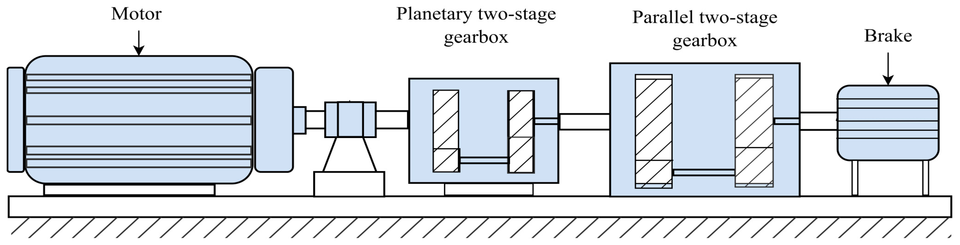
In this paper, a novel hierarchical adaptive wavelet-guided adversarial network with physics-informed regularization (HAWAN-PIR) is proposed. The objective of HAWAN-PIR is to generate high-quality, multiscale time-series vibration signals to enrich the training dataset for a one-dimensional convolutional network (1-D CNN). More importantly, HAWAN-PIR incorporates physics-informed regularization of machinery faults to ensure that the generated signals adhere to known physical knowledge and constraints. The 1-D CNN model autonomously extracts high-level features from the input data and uses these features to predict the health state of the target machinery. The effectiveness of HAWAN-PIR and the associated fault diagnosis process is validated through two experimental studies: motor rolling bearings and planetary gearboxes.
The main contributions of this study can be summarized as follows:
(1)
A hierarchical wavelet-based imbalance severity score is introduced to quantify data imbalance across multiple scales in fault diagnosis datasets.
(2)
A new hierarchical GAN architecture with physics-informed regularization is proposed that uses adaptive wavelet decomposition to generate realistic vibration signals at different scales, significantly enhancing fault diagnosis in rotating machinery.
(3)
A multiscale synthesis quality index is developed to evaluate the quality of the generated fault data. This index assesses the fidelity and realism of synthetic data across different scales.
(4)
A scale-aware dynamic mixing algorithm is presented to optimally integrate synthetic data with real data. This addresses how to effectively combine these datasets.
(5)
In this paper, ablation studies are conducted to verify the effectiveness of the HAWAN-PIR framework. The studies analyze how different components of HAWAN-PIR contribute to the diagnostic performance of the 1-D CNN model.
The subsequent sections of this paper are organized as follows: Section 2 details the proposed method, Section 3 presents the experimental validation and analysis, and Section 4 concludes this paper.

2. The Proposed Method

2.1. Network Architecture of HAWAN-PIR

To address the data imbalance problem and improve fault diagnosis performance, HAWAN-PIR is proposed in this paper. This framework generates additional multiscale time-series vibration signals, which are then utilized by a 1-D CNN for fault pattern recognition. The overall data generation strategy for the fault diagnosis task is depicted in Figure 1.
The network architecture of HAWAN-PIR comprises two main components: the generator and the discriminator, as depicted in Figure 1. The generator is structured as a four-layer network, with layer sizes set to 128, 256, 512, and 1024 units, respectively. The initial layer contains 128 units, which represent the combined dimensions of the noise vector and the label vector. In contrast, the discriminator is structured as a two-layer network, with units configured to 1024, 512, and 1 in each layer. The larger initial layer (i.e., 1024 units) of the discriminator captures complex features from the time series data, whereas the subsequent layers reduce to 512 and then 1 unit to enhance its classification ability. These parameters were determined through a series of iterative experiments.
The objective function of HAWAN-PIR is designed to ensure the generation of realistic and physically consistent synthetic fault data. This function can be mathematically expressed as:
L t o t a l = L a d v + λ 1 L r e c o n + λ 2 L p h y s + λ 3 L s c a l e + λ 4 L e n t r o p y ,
where each component of this objective function serves a specific purpose in maintaining the integrity and quality of the generated data.
The multiscale adversarial loss ( L a d v ) ensures that the generated data are indistinguishable from the real data across different scales. This loss is formulated as:
L a d v = s [ E log D s x s + E [ log ( 1 D s ( G s ( z s ) ) ) ] ] ,
where s represents different scales, D s is the scale-specific discriminator, G s is the scale-specific generator, x s denotes the real data at scale s , and z s is the random noise input at scale s .
The reconstruction loss ( L r e c o n ) ensures that the generator can accurately reconstruct input signals, which can be expressed as:
L r e c o n = x G ( E ( x ) ) 2 ,
where E functions as an encoder that maps real signals into a latent space, whereas G reconstructs the signal from this latent representation.
The physics-informed regularization term ( L p h y s ) enforces physical constraints on the generated signals—emphasizing the features that contain the most relevant fault information—and is tailored for each case study.
The hierarchical structure is fundamentally linked to the wavelet transform, as wavelet decomposition captures multi-resolution features from the vibration signals, organizing these features in a way that prioritizes relevant fault characteristics. This hierarchy allows the model to effectively utilize information at different scales, enhancing diagnostic performance. By structuring the extracted features hierarchically, the model can leverage both general and specific fault-related information, leading to more accurate predictions.
In the case of rolling bearings, the physics-informed regularization can be expressed as:
L p h y s C W R U = i i G z i x 2 ,
where i represents the essential features that characterize the fault conditions in rolling bearings. These features are derived from the physical characteristics of the machinery and include parameters such as fault characteristic frequencies. In this work, we consider three types of bearing faults: inner race faults, outer race faults, and roller or ball faults. The fault characteristic frequency formulas for these types of bearing faults are as follows [30]:
F I R = f r × n 2 1 + d D cos α ,
F O R = f r × n 2 1 d D cos α ,
F B = f r × D 2 d 1 d D 2 c o s 2 α ,
where n is the number of rolling elements, d is the diameter of the rolling element, D is the pitch diameter, F I R , F O R , and F b are the fault characteristic frequencies of the inner race, outer race, and rolling element, respectively, f r is the rotating frequency of the shaft, and α is the load angle relative to the radial plane.
For the planetary gearbox case, the physics-informed regularization can be expressed as:
L p h y s S E U = i φ j G z φ j x 2 ,
where φ j includes features relevant to the gearbox, such as gear mesh frequencies, which are crucial for identifying faults in the gear system. The gear mesh frequency can be calculated as [33]:
F g m = N g 60 . R p D p ,
where N g is the number of teeth on the gear, R p is the rotational speed of the gear in the RPM, and D p is the pitch diameter of the gear.
It is important to clarify that the features i and j do not imply a direct relationship with the process of obtaining harmonic amplitudes through Fast Fourier Transform (FFT). Instead, i and j include essential fault-related features that are extracted based on the physical characteristics of the machinery being analyzed. These features represent various aspects of the vibration signals, such as amplitudes at specific fault characteristic frequencies, which are crucial for diagnosing the health of the machinery.
The multiscale coherence loss ( L s c a l e ) ensures consistency across different scales of the generated signals, which can be expressed as:
L s c a l e = s , t W s G t z W s x 2 ,
where W s represents the wavelet transform applied at scale s . This integration allows for the analysis of signals across multiple scales. The term G t denotes the generator output at scale t . This approach enables the effective capture of temporal and frequency characteristics of the data.
It is important to note that this formulation allows for the measurement of differences between the wavelet-transformed generated signals and the real signals at each scale. By enforcing coherence, the generated output aligns more closely with the characteristics of the real signals across different scales.
Finally, the entropy balancing loss ( L e n t r o p y ) maintains the complexity and information content of the generated signals, which can be expressed as:
L e n t r o p y = H G z | H ( x ) ,
where H is the Shannon entropy. This loss function ensures that the generated signals retain a similar level of complexity and information as the real signals, further enhancing the fidelity of the proposed HAWAN-PIR model.

2.2. Hierarchical Wavelet-Based Imbalance Severity Score

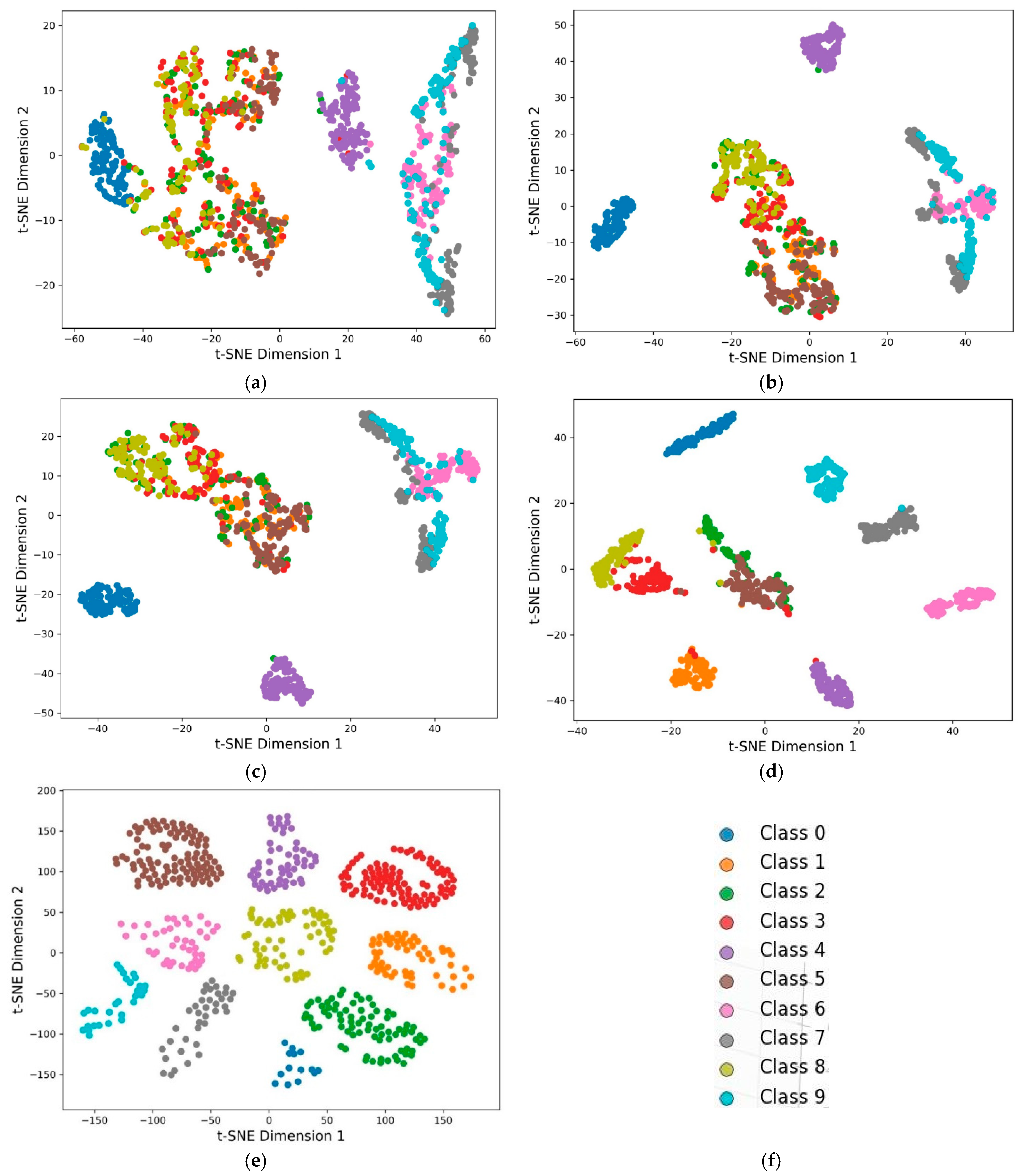
To quantify data imbalance across multiple scales and multiclass problems, the hierarchical wavelet-based imbalance severity score (HWISS) is presented. Particularly, for this work, the total number of classes is ten, i.e., one healthy class and nine fault classes. The HWISS is defined as:
H W I S S = j = 0 9 i = 1 N w i j . R i j ,
where w i j represents the physics-informed weighting for scale i of class j .
The fault-to-normal sample ratio at scale i for class j can be expressed as:
R i j = N u m b e r   o f   f a u l t   s a m p l e s   a t   s c a l e   i   f o r   c l a s s   j N u m b e r   o f   n o r m a l   s a m p l e s ,
Each sample undergoing the wavelet transform generates signals at N different scales. The dependence of R i j on i arises because each scale captures different levels of detail in the vibration signals, leading to variations in the number of fault samples captured at each scale. This reflects the hierarchical nature of the vibration signals being analyzed.
The weighting w i j is critical as it emphasizes the importance of features extracted at each scale for fault diagnosis. These weights are determined based on the relevance of the physical features, such as fault characteristic frequencies, to the specific fault conditions being analyzed. By incorporating these physics-informed weights, the HWISS provides a comprehensive measure of imbalance that considers both the scale-specific ratios R i j and the hierarchical structure of the data. A higher HWISS indicates a more severe imbalance across the scales, which can significantly impact fault diagnosis.

2.3. Comprehensive Multiscale Synthesis Quality Index

The quality of generated data is a critical factor that impacts classification accuracy in the context of imbalanced diagnosis. To evaluate the quality of the generated data, the comprehensive multiscale synthesis quality index (CMSQI) is proposed in this study, which can be expressed as:
C M S Q I = α · W D S + β · P I S F M + γ · C B I M ,
This index integrates three main components:
(1)
The wavelet-based discriminative score (WDS) measures how well the synthetic data align with the real data in the wavelet domain;
(2)
The physics-informed signal fidelity measure (PISFM) evaluates how well the synthetic data adhere to the known physical principles of rotating machinery;
(3)
The class balance improvement metric (CBIM) quantifies how much the synthetic data improve the balance between fault and healthy classes.
The weights α , β , and γ indicate the relative importance of each component in the overall quality evaluation. A higher CMSQI score signifies better quality of the generated data.

2.4. Scale-Aware Dynamic Mixing Algorithm

The scale-aware dynamic mixing (SADM) algorithm optimizes the integration of synthetic and real data for training 1-D CNN classifiers. The mixing ratio (MR) for each scale i can be calculated as:
M R i = f H W I S S i , C M S Q I i , C N N p e r f i ,
where H W I S S i is the imbalance severity score, C M S Q I i is the synthesis quality index, and C N N p e r f _ i is a measure of the performance of the 1-D CNN on scale i data. If H W I S S i is high, C M S Q I i is high, and C N N p e r f _ i is low, the function f might return a high M R i to include more synthetic data. Conversely, if H W I S S i is low, C M S Q I i is low, and C N N p e r f _ i is high, f might return a low M R i to rely more on real data.
This adaptive mixing strategy ensures that more synthetic data are utilized where the imbalance is significant, higher-quality synthetic data are prioritized, and the mixing ratio is adjusted based on CNN performance. This creates a feedback loop that optimizes data generation for the specific classification task.

2.5. Training and Fault Classification Procedures

As mentioned earlier, the HAWAN-PIR framework is used to extend the training samples, and these samples, in combination with the real data, are then utilized by a 1-D CNN for fault pattern recognition.
The training process begins with the initialization of both the generator G and the discriminator D networks, which are set with random weights to facilitate effective learning during training iterations. In each iteration, real data x and random noise z are sampled. The generator uses this noise to create synthetic data G(z). The training involves calculating a total loss L t o t a l , which includes the following components: L a d v , L r e c o n , L p h y s , L s c a l e , and L e n t r o p y . The parameters of the discriminator are updated to minimize L a d v , whereas the parameters of the generator are adjusted to minimize L t o t a l . Thus, the fault data are generated.
Once the synthetic samples are generated, periodic assessments using the CMSQI metrics are performed to evaluate the quality of the synthetic data. After these evaluations, the SADM algorithm is applied to create an optimally mixed dataset of real and synthetic data for each scale.
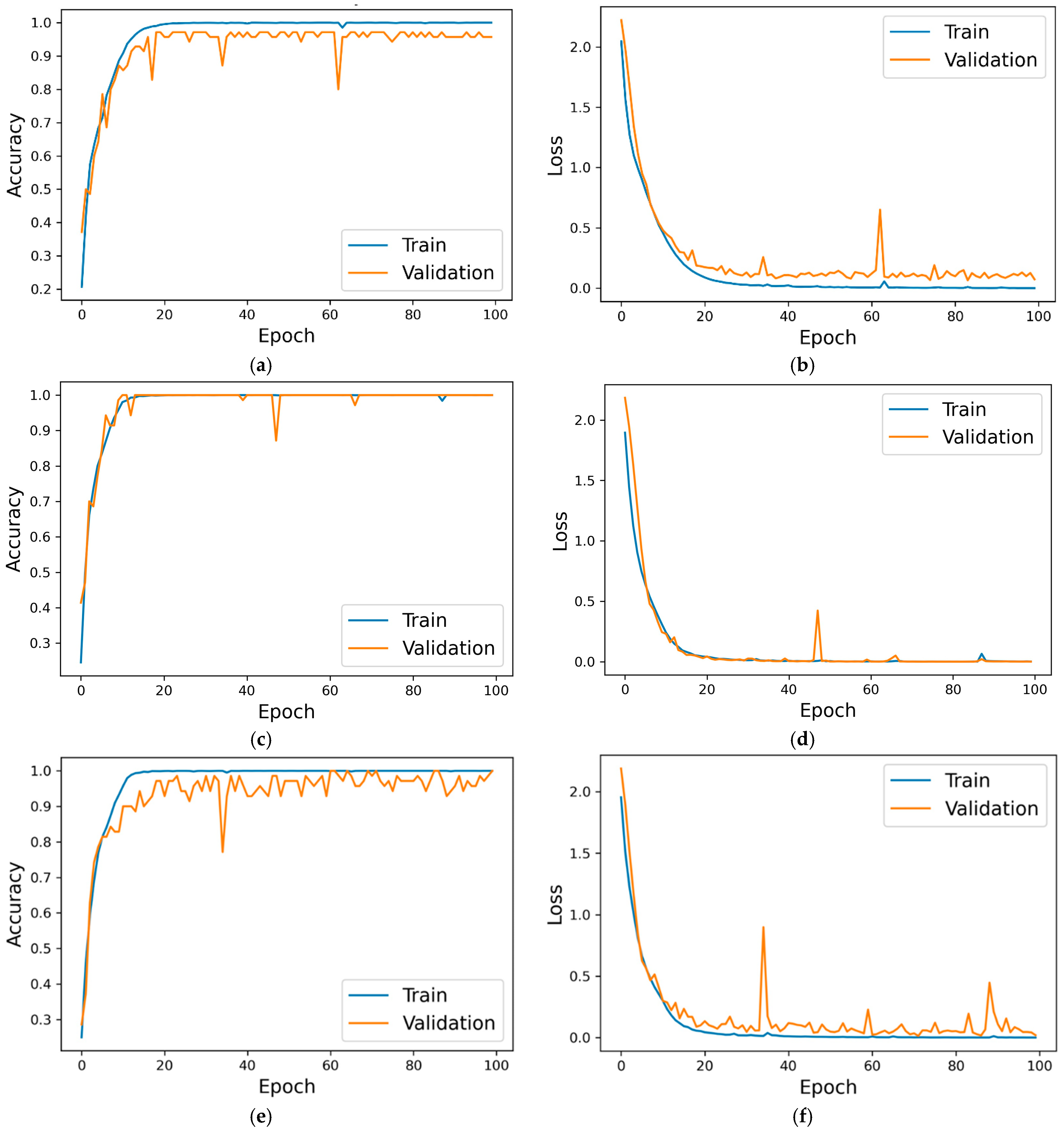
The mixed data are then split into three sets: training, validation, and testing. The 1-D CNN is trained on the training set, and a separate validation set is used to determine if overfitting occurs. The network architecture of the 1-D CNN is shown in Figure 2. Details regarding each layer type in the architecture can be found in our previously published work [34], which this study further extends.
The network parameters and training hyperparameters of the 1-D CNN are detailed in Table 1 and Table 2, respectively. These parameters and hyperparameters were determined through a series of experiments.
Once the training process is complete, the diagnostic capability of the 1-D CNN is rigorously evaluated via a separate test set. This evaluation is essential for determining the ability of the model to generalize to unseen data.
The overall flowchart in Figure 3 shows the proposed methodology for data generation and fault diagnosis in the rotating machines used in this study. This flowchart details steps such as data imbalance evaluation, synthetic data generation, synthetic data quality assessment, integration of the synthetic data with the real data, and partitioning of the mixed data for fault diagnosis.

3. Experimental Validation

In this section, we present two case studies to validate the effectiveness of the HAWAN-PIR framework and the subsequent fault diagnosis process: bearing data from Case Western Reserve University (CWRU) [36] and gearbox data from Southeast University (SEU), China [37].

3.1. Case 1: Rolling Bearing Data from CWRU

3.1.1. CWRU Rolling Bearing Data Description

The rolling bearing vibration data used in this study were obtained from the CWRU Bearing Data Center [36], which is renowned for its extensive collection of vibration data for fault diagnosis in rolling bearings. The data were collected from a motor bearing test rig, as shown in Figure 4.
In this work, the vibration data recorded from the driving end of the test rig at a sampling rate of 12 kHz were chosen for experimental verification. The data correspond to four different load conditions: 0 hp, 1 hp, 2 hp, and 3 hp. Within each load condition, four different types of health states were considered: normal, inner race fault, outer race fault, and rolling bearing ball fault. For each fault type, faults with diameters of 0.007, 0.014, and 0.021 inches were identified. The locations of these faults are shown in Figure 5.
For this analysis, four datasets labeled A, B, C, and D were prepared, corresponding to four load conditions (0, 1, 2, and 3 hp, respectively). Each dataset consisted of ten states, namely, nine fault states and one healthy state, which were labeled from 0 to 9. To account for varying working conditions, a combined dataset (i.e., A/B/C/D) was created that integrates all four individual datasets.
Considering a sampling frequency of 12 kHz and a motor speed of 1797 rpm at no load, the sample length needs to be greater than 400, which approximates the number of samples for a full rotation of the bearing. However, for this study, a length of 2048 was chosen to align with the existing research [38,39].

3.1.2. Data Imbalance Level in CWRU Rolling Bearing Data

To examine the data generation performance of HAWAN-PIR, it is crucial to assess the level of imbalance. The extent of data imbalance was evaluated via the HWISS, which measures fault-to-normal sample ratios at various decomposition scales. The HWISS was calculated for each individual dataset—A, B, C, and D—as well as for the combined dataset (i.e., A/B/C/D), as presented in Table 3.
The results in Table 3 reveal varying levels of data imbalance across the datasets. Dataset A has a moderate HWISS of 0.75 and a fault-to-normal ratio of 1:10, indicating a fair representation of fault classes. Dataset B has the lowest HWISS of 0.68 and a ratio of 1:12, suggesting that a better balance could aid model training. In contrast, Dataset C displays the highest HWISS of 0.82 and a ratio of 1:8, which may hinder the identification of less frequent faults. Dataset D is similar to Dataset A, with an HWISS of 0.70 and a ratio of 1:11. The combined dataset reflects a significant overall imbalance, with an HWISS of 0.77 and a ratio of 1:9. This imbalance was intentionally created to simulate real-world conditions.
To further illustrate these results, the distributions of the ten classes (i.e., one healthy class and nine fault classes) in each dataset are depicted in Figure 6. This visualization shows the fault-to-normal ratios and their corresponding percentage distributions. Each sample consists of 2048 data points.
These results reveal varying levels of imbalance across the datasets, which poses challenges when training effective deep learning models. This underscores the necessity of strategies such as data augmentation to improve the representation of less frequent fault classes and to enhance the performance and reliability of fault diagnosis models in real-world applications.

3.1.3. Data Generation and Quality Analysis for CWRU Rolling Bearing Data

Once a high level of data imbalance was confirmed, the proposed HAWAN-PIR was employed to generate artificial fault samples. The quality of the synthetic fault data produced by HAWAN-PIR was rigorously evaluated via the CMSQI. This index assesses how closely synthetic data align with real data in terms of fidelity and realism. The CMSQI values obtained for the datasets are as follows: Dataset A received a score of 0.84, Dataset B achieved 0.88, Dataset C scored 0.85, Dataset D recorded a score of 0.87, and the combined dataset had an overall score of 0.86.
CMSQI scores above 0.80 are generally considered indicative of high fidelity and realism. Thus, the results from these evaluations indicate that the generated samples effectively retain the essential features of real-world faults. Specifically, the synthetic data mirror the frequency characteristics observed under actual fault conditions, which is crucial for ensuring accurate fault detection. Furthermore, the timing and sequence of events in the synthetic data closely reflected those found in real-world scenarios. This alignment significantly enhances the ability of the model to recognize patterns indicative of faults. The amplitude levels present in the synthetic samples corresponded well to those encountered in real faults, which is vital for enabling the models to be generalized effectively to actual operating conditions. These results affirm the effectiveness of HAWAN-PIR in generating high-quality synthetic data.

3.1.4. Integration of Synthetic and Real Data for CWRU Rolling Bearing Data

After the artificial data were generated via HAWAN-PIR for fault diagnosis, it was necessary to integrate the synthetic data with the real data to enrich the training dataset. The integration was achieved through the SADM algorithm. This algorithm dynamically determines the mixing ratios for each dataset based on metrics that reflect varying levels of imbalance and data quality, as summarized in Table 4.
As presented in Table 4, the mixing ratios range from 0.65 to 0.80, indicating a strong reliance on the synthetic data. For example, Dataset B has the highest ratio of 0.80, meaning that it contains 80% synthetic data and 20% real data. On the other hand, Dataset D has the lowest ratio at 0.65, with 65% synthetic data and 35% real data. This adaptive approach proves how the SADM algorithm adjusts the mixing ratios based on the specific characteristics of each dataset. This allows for more synthetic data to be used in cases where there is significant class imbalance. The integration of synthetic and real data through the SADM algorithm is expected to improve fault diagnosis performance. This approach not only increases the accuracy of the model but also enhances its robustness against different fault types.

3.1.5. Diagnosis Results for CWRU Rolling Bearing Data

The combined data were input into the 1-D CNN for feature extraction and fault classification. To evaluate the efficacy of the 1-D CNN, the analysis began with the training curves. In this case, the data hp = 0, 2, and 0/1/2/3 were used as representatives. Figure 7 shows the training curves for Dataset A, Dataset C, and the combined dataset A/B/C/D, which utilized both the real and fake data generated via HAWAN-PIR.
As shown in Figure 7, for Dataset A, the 1-D CNN model achieved a training accuracy of 98% within the first 30 epochs and stabilized at approximately 100%. For Dataset C, the training accuracy of the model sharply increased during the first 10 epochs and reached a stable diagnosis accuracy of approximately 100% by the 25th epoch. When all the datasets were combined, the model attained an overall training accuracy of approximately 99%. This trend was consistent with the results from the other datasets. Furthermore, the loss curves of training approached zero across all datasets. These results indicate that the integration of the fake data with the real data effectively enhances the training performance of the 1-D CNN, with no evidence of overfitting.
Following the training analysis, the fault diagnosis accuracy for each dataset was evaluated via a testing set. This evaluation was conducted for ten trials to minimize randomness and ensure the reliability of the results. The average diagnostic accuracies for each dataset are presented in Table 5.
The results in Table 5 validated a notable improvement in diagnostic accuracy following the integration of the synthetic data. For Dataset A, the model attained a testing accuracy of 80.35% with a standard deviation of ±2.54 when trained solely on the real data. After incorporating the synthetic data, the accuracy increased to 95.13%, accompanied by a reduced standard deviation of ±0.83. Similarly, Dataset B showed an increase in accuracy from 81.43% (±3.67) when the real data were used to 96.57% (±0.69) when the integrated data were used. For Dataset C, the accuracy improved from 78.57% (±2.57) to 96.34% (±0.77), and for Dataset D, it increased from 79.66% (±3.34) to 96.41% (±0.56). The combined datasets also reflected this trend, with the accuracy increasing from 80.94% (±4.66) when the real data were used to 94.85% (±1.75) when the integrated data were used. The higher standard deviations in the real data scenarios indicate challenges related to the imbalance in fault classes, which hinders effective learning. These results validate the difficulties faced by deep learning models when trained exclusively on imbalanced real data, as certain fault classes were underrepresented, resulting in a bias toward the majority class (i.e., healthy samples in this case). In contrast, the integration of the synthetic data enabled the 1-D CNN model to identify faults more effectively, resulting in improved accuracy and reliability.
To further verify the performance of the diagnostic model on the testing set, confusion matrices for each dataset were analyzed. Figure 8 presents the confusion matrices of the 1-D CNN for the bearing datasets.
As shown in Figure 8, the diagnosis model successfully classified health conditions across all datasets. In Dataset A, the model accurately identified a significant proportion of health states. Although Dataset C presented commendable true positive rates, it experienced slightly more false positives than Dataset A did. For the combined dataset (i.e., Datasets A/B/C/D), the confusion matrix indicated a similar trend, with high true positive rates for fault detection and no false positives for healthy states across all datasets. This consistent performance is largely attributed to the synthetic data generated by the HAWAN-PIR framework, which enriched the training dataset and improved the diagnostic accuracy of the 1-D CNN model. More specifically, the incorporation of physics-informed regularization in HAWAN-PIR minimizes false positives, particularly in situations where the model might incorrectly predict rolling bearing faults.
Finally, to intuitively show the effectiveness of HAWAN-PIR in generating fault data samples and the 1-D CNN for fault classification, this study employs the t-SNE technique. This approach allows for the evaluation of the quality of the synthetic data and the ability of the diagnosis model to differentiate between various classes within the dataset. Figure 9 shows the t-SNE plots for the combined dataset (i.e., A/B/C/D), which serves as a representative overview of the other datasets across all load conditions.
The t-SNE plots demonstrate an improvement in the separation of clusters from layer to layer. This enhancement can be attributed to the sufficient number of training samples, which comprise both the real and fake data. As the 1-D CNN progresses through these layers, it effectively learns to extract more relevant features, leading to better differentiation between fault types and healthy states. In particular, the clear clustering observed in Dense_1 and Dense_2 suggests that the diagnosis model has successfully captured complex relationships within the data. These findings emphasize the importance of both the architecture of the network and the quality of the training data in achieving effective fault diagnosis.

3.2. Case 2: Planetary Gearbox Data from the SEU

3.2.1. SEU Planetary Gearbox Data Description

To further verify the effectiveness of the HAWAN-PIR method in generating fault samples and the subsequent fault diagnosis process via the 1-D CNN, other imbalanced gearbox data were utilized. The vibration signals were collected from a planetary gearbox setup at Southeast University (SEU), China [37]. Figure 10 shows a schematic of the SEU experimental setup used to collect the vibration.
This study focused on two distinct configurations characterized by specific rotating speed–load conditions: 20 Hz-0 V and 30 Hz-2 V. Within these conditions, ten health states were examined for both bearings and gearboxes, as detailed in Table 6.
To support the analysis, two main datasets were prepared, designated A and B, which correspond to the operational conditions of 20 Hz-0 V and 30 Hz-2 V, respectively. Each dataset consisted of five distinct health conditions: four fault states and one healthy state. Furthermore, a more complex dataset labeled A/B was developed to improve the robustness of the analysis. This dataset not only accommodated varying working conditions but also incorporated compound faults to provide a comprehensive basis for evaluating the diagnosis model.

3.2.2. Data Imbalance Level in SEU Planetary Gearbox Data

Similar to the previous case, the extent of data imbalance was assessed via the HWISS, which evaluates fault-to-normal sample ratios at various decomposition scales. The HWISS was calculated for each dataset—A and B—as well as for the combined dataset (i.e., A/B), as presented in Table 7.
These results indicate class imbalance challenges in each dataset, particularly due to the lower representation of fault conditions compared with healthy states. Such disparities can hinder the ability of the 1-D CNN to learn effectively, resulting in inaccuracies in fault classification. Therefore, addressing this imbalance through HAWAN-PIR will improve the reliability of the diagnosis.

3.2.3. Data Generation and Quality Analysis for SEU Planetary Gearbox Data

Similarly, the CMSQI was used to evaluate the quality of the synthetic fault data generated by HAWAN-PIR. The CMSQI scores for the synthetic data were as follows: 0.87 for Dataset A, 0.85 for Dataset B, and 0.88 for the combined dataset.
For Dataset A, the score of 0.87 indicates that the synthetic samples for the 20 Hz-0 V condition closely resemble real operational dynamics. In comparison, Dataset B received a score of 0.85, which reflects slightly lower fidelity for the 30 Hz-2 V condition but still shows that the synthetic data are representative of real-world scenarios. The combined dataset achieved the highest score of 0.88. These scores further confirm the effectiveness of the HAWAN-PIR framework in producing high-quality synthetic data for model training.

3.2.4. Integration of Synthetic and Real Data for SEU Planetary Gearbox Data

As extended samples, the artificial fault data were combined with the real samples and then trained via the 1-D CNN model. This integration was accomplished through the SADM algorithm, which aims to address imbalance by increasing the sample size. The algorithm dynamically determines the mixing ratios for each dataset based on metrics that reflect varying levels of imbalance and data quality. The calculated mixing ratios for each dataset are summarized in Table 8.
The mixing ratios range from 0.75 to 0.80, indicating a significant reliance on the synthetic data. For example, Dataset B has the highest ratio of 0.80, consisting of 80% synthetic data and 20% real data, whereas Dataset A has a ratio of 0.75. This strategy effectively addresses class imbalance and enhances the training process of the diagnosis model. By incorporating a greater proportion of the synthetic data, the model is better equipped to learn from diverse fault conditions, ultimately improving its diagnostic accuracy and reliability in real-world applications.

3.2.5. Diagnosis Results for SEU Planetary Gearbox Data

After generating the synthetic fault data and evaluating their extent and quality, the fault diagnosis results obtained from the 1-D CNN were evaluated. The experiments were conducted over ten trials to minimize the effects of randomness. Figure 11 shows the training curves for each dataset from a single trial.
As shown in Figure 11, the training curves confirm that the 1-D CNN steadily approaches a training accuracy of nearly 100% across all gearbox datasets. The training loss curves decrease with an increasing number of iterations and approach zero after approximately 30 epochs. This consistent training performance indicates that the model effectively learns the underlying patterns in the data, signifying a successful training process.
The diagnostic accuracies of the 1-D CNN were evaluated over ten trials using the testing set. For Dataset A, which corresponds to the 20 Hz-0 V condition, the model achieved an average diagnostic accuracy of 98.67% with a standard deviation of 0.27%. In the case of Dataset B, which represents the 30 Hz-2 V condition, the model attained an average accuracy of 97.34% with a standard deviation of 0.18%. When Datasets A and B were combined, the model yielded an accuracy of 96.73%, with a standard deviation of 2.25%. In addition, under imbalanced ratios, the diagnostic accuracies decreased significantly—by approximately 15%. The analyses indicate that the proposed HAWAN-PIR not only generates relevant synthetic samples that enhance the training process but also improves the testing accuracy of the 1-D CNN.
Figure 12 shows the confusion matrices for each dataset. As shown, the diagnosis model effectively classifies all health conditions, with only a few misclassifications. The matrices indicate a reduction in false positives across all datasets, attributed to the incorporation of physics-informed regularization in HAWAN-PIR. Thus, the proposed HAWAN-PIR significantly improves the diagnostic accuracy of the 1-D CNN.
Finally, as in the previous case, the extracted features were analyzed via t-SNE to provide visual insights into the testing dataset. This technique maps high-dimensional features into a two-dimensional space, with the results shown in Figure 13, where each color represents a distinct health state of the gearboxes.
As shown in Figure 13, the t-SNE plots reveal improved cluster separation from layer to layer. In the initial layers (Conv1D_1, Conv1D_2, and Conv1D_3), the extracted features are mixed together. However, as shown in Figure 13d,e, as the model progresses to the dense layers (Dense_1 and Dense_2), the clustering becomes much clearer. These results clearly indicate that the 1-D CNN has learned to represent the data in a way that facilitates accurate fault diagnosis.

3.3. Ablation Study

This section describes an ablation study conducted to evaluate the contributions of components of the HAWAN-PIR framework to the 1-D CNN model. More specifically, this study evaluated the impact of omitting three main components, i.e., wavelet decomposition, physics-informed regularization, and hierarchical structure, on diagnostic accuracy. The results of this ablation study, which utilized the combined data from both the CWRU rolling bearing dataset and the SEU planetary gearbox dataset, are presented in Table 9.
As shown in Table 9, the ablation study demonstrates significant improvements with the HAWAN-PIR framework. The original 1-D CNN model achieved accuracies of 80.94% for the rolling bearing dataset and 79.77% for the planetary gearbox dataset. After HAWAN-PIR was employed for data generation, these accuracies increased to 94.85% and 96.73%, respectively. This underscores the critical role of synthetic samples in enhancing the robustness of the diagnostic model, particularly in scenarios with limited fault data.
Removing wavelet decomposition resulted in decreased accuracies of 91.45% for the CWRU dataset and 92.67% for the SEU dataset, underscoring its importance in feature extraction. The wavelet transform plays a crucial role in capturing multi-resolution features that enhance the hierarchical structure, allowing for better organization and prioritization of fault characteristics.
Similarly, omitting physics-informed regularization led to further decreases to 89.73% for the CWRU dataset and 90.05% for the SEU dataset, suggesting that domain knowledge significantly enhances model generalizability. Simplifying the hierarchical structure also resulted in accuracies of 90.29% for CWRU and 91.34% for SEU, emphasizing the importance of a well-structured model that works in conjunction with the wavelet transform.
Finally, excluding the integration of synthetic data reduced the accuracy to 92.67% for the CWRU dataset and 93% for the SEU dataset. Overall, these results confirm the significance of wavelet decomposition, physics-informed regularization, hierarchical structure, and synthetic data integration in improving fault diagnosis capabilities, especially in the context of imbalanced data.

4. Conclusions

In this paper, a new hierarchical adaptive wavelet-guided adversarial network with a physics-informed regularization (HAWAN-PIR) framework is proposed to overcome the issue of imbalanced fault data and enhance the diagnostic accuracy of rotating machines, particularly for components such as bearings and gearboxes. The framework generates high-quality artificial fault data in the time domain through multiscale wavelet decomposition and is the first to incorporate relevant fault knowledge or physical principles.
Initially, the hierarchical wavelet-based imbalance severity score (HWISS) was employed to evaluate the level of data imbalance. Next, the HAWAN-PIR framework was employed to generate high-quality data at different scales, which were then evaluated via a comprehensive multiscale synthesis quality index (CMSQI). Furthermore, a scale-aware dynamic mixing algorithm was introduced to effectively combine synthetic and real data, thereby increasing the training dataset for the 1-D CNN. Finally, two experimental studies—rolling bearings and planetary gearboxes—were conducted to validate the effectiveness of the HAWAN-PIR framework and its fault diagnosis process. From the analysis of these cases, the following conclusions can be drawn:
  • The HWISS values indicate varying levels of data imbalance, with rolling bearings scoring from 0.68 to 0.82 and planetary gearboxes scoring from 0.68 to 0.75. These results underscore the significant imbalances present and prove the need for a data generation model (i.e., HAWAN-PIR in this case) to improve the diagnostic accuracy of deep learning models.
  • The CMSQI scores exceeded 0.80 in both case studies. This proves that the data generated by HAWAN-PIR have high fidelity and realism.
  • The mixing ratios for the bearing datasets range from 0.65 to 0.80, whereas those for the gearbox datasets range from 0.75 to 0.80. These ratios reflect a balance between synthetic and real data.
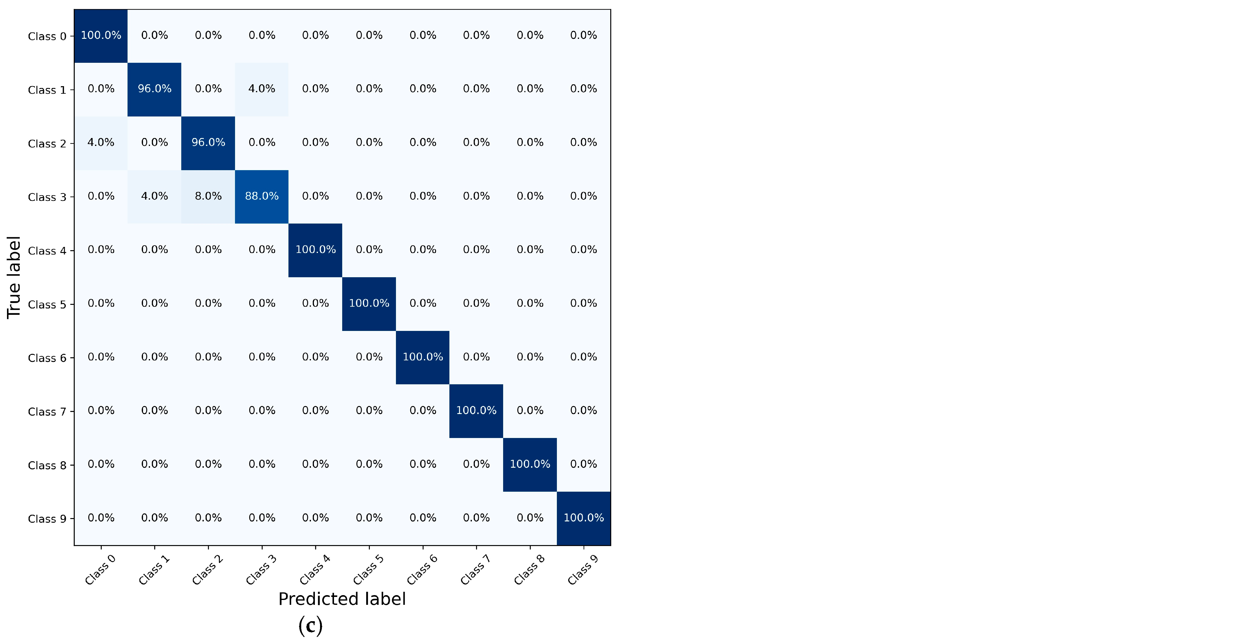
  • The diagnosis accuracy of the fault diagnosis model based on the 1-D CNN shows significant improvements, with a 17% increase for the bearing datasets and a 15% increase for the gearbox datasets. This advance is attributed to the high quality of the data generated via HAWAN-PIR.
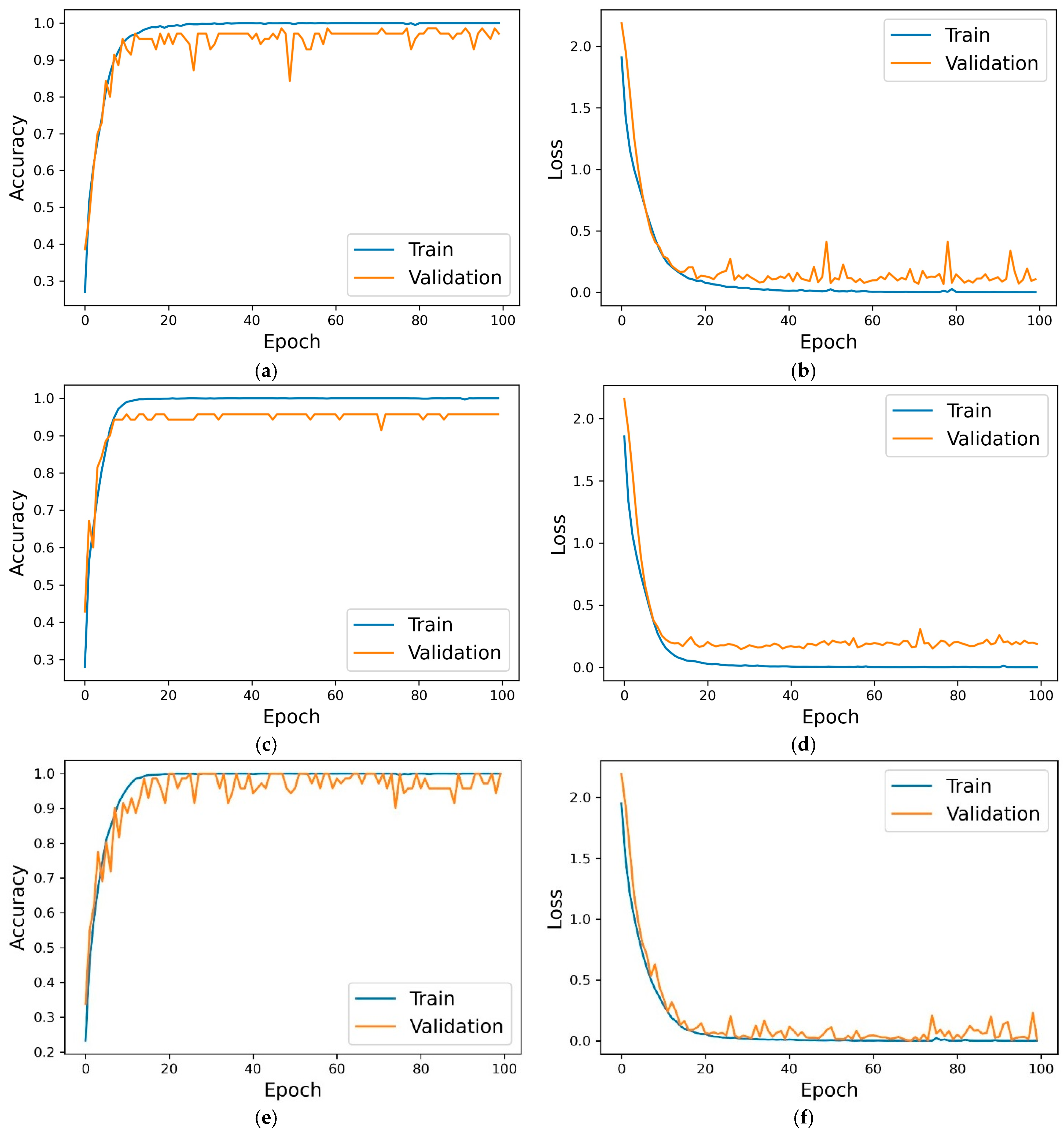
  • Finally, the ablation study evaluated the contributions of each component of HAWAN-PIR—wavelet decomposition, physics-informed regularization, and hierarchical structure—to the 1-D CNN model. The integration of these components significantly improved the accuracy from 80.94% to 94.85% for the CWRU bearing dataset and from 79.77% to 96.73% for the SEU gearbox dataset, even under varying load conditions.
In the two case studies, the effectiveness of the HAWAN-PIR framework was validated solely through the 1-D CNN. However, other deep learning models remain unexamined. Therefore, for future work, the authors plan to investigate the applicability of the HAWAN-PIR framework to increase the diagnostic accuracy of these other models. Additionally, this study considers limited physics principles for the rolling bearing and gearbox cases, specifically focusing on fault characteristic frequencies for the rolling bearing case and gear mesh frequencies for the gearbox case. In the future, the authors intend to explore the integration of additional physical principles, such as material properties, thermal effects, and dynamic behavior, to further improve the diagnostic performance of deep learning models in real-world applications.

Author Contributions

Conceptualization, F.K.; methodology, F.K.; software, F.K.; validation, F.K., D.E.W. and H.S.G.; resources, D.E.W. and H.S.G.; data curation, F.K.; writing—original draft preparation, F.K.; writing—review and editing, D.E.W. and H.S.G.; supervision, D.E.W.; project administration, D.E.W.; funding acquisition, D.E.W. All authors have read and agreed to the published version of the manuscript.

Funding

This research was funded by the Artificial Intelligence and Robotics Center of Excellence at Addis Ababa Science and Technology University, grant number IGP012/2023.

Data Availability Statement

The original data presented in this study are openly available at Case Western Reserve University Bearing Data Center (https://engineering.case.edu/bearingdatacenter (accessed on 29 August 2024)) and on GitHub (https://github.com/cathysiyu/Mechanical-datasets (accessed on 3 September 2024)).

Acknowledgments

The authors wish to gratefully acknowledge the Artificial Intelligence and Robotics Center of Excellence at Addis Ababa Science and Technology University, Ethiopia, for providing the space and necessary equipment for this work.

Conflicts of Interest

The authors declare no conflicts of interest.

References

  1. Liang, P.; Deng, C.; Wu, J.; Yang, Z. Intelligent fault diagnosis of rotating machinery via wavelet transform, generative adversarial nets and convolutional neural network. Meas. J. Int. Meas. Confed. 2020, 159, 107768. [Google Scholar] [CrossRef]
  2. Kibrete, F.; Woldemichael, D.E. Applications of Artificial Intelligence for Fault Diagnosis of Rotating Machines: A Review. In Lecture Notes of the Institute for Computer Sciences, Social-Informatics and Telecommunications Engineering, LNICST; Springer: Cham, Switzerland, 2023; pp. 41–62. [Google Scholar] [CrossRef]
  3. Li, X.; Yan, L.; Ye, P.; Wu, J.; Hu, J. Enhanced Fault Diagnosis in Time-series Data by Deep Learning. In Proceedings of the 2023 9th International Conference on Big Data and Information Analytics, BigDIA 2023, Haikou, China, 15–17 December 2023; Institute of Electrical and Electronics Engineers Inc.: New York, NY, USA, 2023; pp. 95–99. [Google Scholar] [CrossRef]
  4. Iqbal, M.; Madan, A.K. Artificial Intelligence-Based Bearing Fault Diagnosis of Rotating Machine to Improve the Safety of Power System. In Lecture Notes in Electrical Engineering; Springer: Singapore, 2024; pp. 933–942. [Google Scholar] [CrossRef]
  5. Brito, L.C.; Susto, G.A.; Brito, J.N.; Duarte, M.A.V. Fault Diagnosis using eXplainable AI: A transfer learning-based approach for rotating machinery exploiting augmented synthetic data. Expert Syst. Appl. 2023, 232, 120860. [Google Scholar] [CrossRef]
  6. Su, H.; Xiang, L.; Hu, A. Application of deep learning to fault diagnosis of rotating machineries. Measurement Science and Technology. Meas. Sci. Technol. 2024, 35, 042003. [Google Scholar] [CrossRef]
  7. Fu, W.; Yang, K.; Wen, B.; Shan, Y.; Li, S.; Zheng, B. Rotating Machinery Fault Diagnosis with Limited Multisensor Fusion Samples by Fused Attention-Guided Wasserstein GAN. Symmetry 2024, 16, 285. [Google Scholar] [CrossRef]
  8. Hu, B.; Liu, J.; Zhao, R.; Xu, Y.; Huo, T. A New Fault Diagnosis Method for Unbalanced Data Based on 1DCNN and L2-SVM. Appl. Sci. 2022, 12, 9880. [Google Scholar] [CrossRef]
  9. Mathew, J.; Pang, C.K.; Luo, M.; Leong, W.H. Classification of Imbalanced Data by Oversampling in Kernel Space of Support Vector Machines. IEEE Trans. Neural Netw. Learn. Syst. 2018, 29, 4065–4076. [Google Scholar] [CrossRef]
  10. Zhang, Y.; Li, X.; Gao, L.; Wang, L.; Wen, L. Imbalanced data fault diagnosis of rotating machinery using synthetic oversampling and feature learning. J. Manuf. Syst. 2018, 48, 34–50. [Google Scholar] [CrossRef]
  11. Duan, F.; Zhang, S.; Yan, Y.; Cai, Z. An Oversampling Method of Unbalanced Data for Mechanical Fault Diagnosis Based on MeanRadius-SMOTE. Sensors 2022, 22, 5166. [Google Scholar] [CrossRef]
  12. Wang, J.; Wei, J.; Huang, H.; Wen, H.; Yuan, Y.; Chen, H.; Wu, R.; Wu, J. IMWMOTE: A novel oversampling technique for fault diagnosis in heterogeneous imbalanced data. Expert Syst. Appl. 2024, 251, 123987. [Google Scholar] [CrossRef]
  13. Mao, W.; He, L.; Yan, Y.; Wang, J. Online sequential prediction of bearings imbalanced fault diagnosis by extreme learning machine. Mech. Syst. Signal Process. 2017, 83, 450–473. [Google Scholar] [CrossRef]
  14. He, Z.; Shao, H.; Wang, P.; Lin, J.J.; Cheng, J.; Yang, Y. Deep transfer multi-wavelet auto-encoder for intelligent fault diagnosis of gearbox with few target training samples. Knowl.-Based Syst. 2020, 191, 105313. [Google Scholar] [CrossRef]
  15. Zhao, B.; Zhang, X.; Li, H.; Yang, Z. Intelligent fault diagnosis of rolling bearings based on normalized CNN considering data imbalance and variable working conditions. Knowl.-Based Syst. 2020, 199, 105971. [Google Scholar] [CrossRef]
  16. Jia, F.; Lei, Y.; Lu, N.; Xing, S. Deep normalized convolutional neural network for imbalanced fault classification of machinery and its understanding via visualization. Mech. Syst. Signal Process. 2018, 110, 349–367. [Google Scholar] [CrossRef]
  17. Goodfellow, I.; Pouget-Abadie, J.; Mirza, M.; Xu, B.; Warde-Farley, D.; Ozair, S.; Courville, A.; Bengio, Y. Generative adversarial networks. Commun. ACM 2020, 63, 139–144. [Google Scholar] [CrossRef]
  18. Wang, Z.; Wang, J.; Wang, Y. An intelligent diagnosis scheme based on generative adversarial learning deep neural networks and its application to planetary gearbox fault pattern recognition. Neurocomputing 2018, 310, 213–222. [Google Scholar] [CrossRef]
  19. Mao, W.; Liu, Y.; Ding, L.; Li, Y. Imbalanced fault diagnosis of rolling bearing based on generative adversarial network: A comparative study. IEEE Access 2019, 7, 9515–9530. [Google Scholar] [CrossRef]
  20. Wang, J.; Han, B.; Bao, H.; Wang, M.; Chu, Z.; Shen, Y. Data augment method for machine fault diagnosis using conditional generative adversarial networks. Proc. Inst. Mech. Eng. Part D J. Automob. Eng. 2020, 234, 2719–2727. [Google Scholar] [CrossRef]
  21. Douzas, G.; Bacao, F. Effective data generation for imbalanced learning using conditional generative adversarial networks. Expert Syst. Appl. 2018, 91, 464–471. [Google Scholar] [CrossRef]
  22. Liu, S.; Jiang, H.; Wu, Z.; Liu, Y.; Zhu, K. Machine fault diagnosis with small sample based on variational information constrained generative adversarial network. Adv. Eng. Inform. 2022, 54, 101762. [Google Scholar] [CrossRef]
  23. Wang, J.; Li, S.; Han, B.; An, Z.; Bao, H.; Ji, S. Generalization of Deep Neural Networks for Imbalanced Fault Classification of Machinery Using Generative Adversarial Networks. IEEE Access 2019, 7, 111168–111180. [Google Scholar] [CrossRef]
  24. Gao, X.; Deng, F.; Yue, X. Data augmentation in fault diagnosis based on the Wasserstein generative adversarial network with gradient penalty. Neurocomputing 2020, 396, 487–494. [Google Scholar] [CrossRef]
  25. Zheng, M.; Li, T.; Zhu, R.; Tang, Y.; Tang, M.; Lin, L.; Ma, Z. Conditional Wasserstein generative adversarial network-gradient penalty-based approach to alleviating imbalanced data classification. Inf. Sci. 2020, 512, 1009–1023. [Google Scholar] [CrossRef]
  26. Zhang, K.; Chen, Q.; Chen, J.; He, S.; Li, F.; Zhou, Z. A multi-module generative adversarial network augmented with adaptive decoupling strategy for intelligent fault diagnosis of machines with small sample. Knowl.-Based Syst. 2022, 239, 107980. [Google Scholar] [CrossRef]
  27. Liu, S.; Jiang, H.; Wu, Z.; Li, X. Data synthesis using deep feature enhanced generative adversarial networks for rolling bearing imbalanced fault diagnosis. Mech. Syst. Signal Process. 2022, 163, 108139. [Google Scholar] [CrossRef]
  28. Qin, Z.; Huang, F.; Pan, J.; Niu, J.; Qin, H. Improved Generative Adversarial Network for Bearing Fault Diagnosis with a Small Number of Data and Unbalanced Data. Symmetry 2024, 16, 358. [Google Scholar] [CrossRef]
  29. Sadoughi, M.; Hu, C. Physics-Based Convolutional Neural Network for Fault Diagnosis of Rolling Element Bearings. IEEE Sens. J. 2019, 19, 4181–4192. [Google Scholar] [CrossRef]
  30. Shen, S.; Lu, H.; Sadoughi, M.; Hu, C.; Nemani, V.; Thelen, A.; Webster, K.; Darr, M.; Sidon, J.; Kenny, S. A physics-informed deep learning approach for bearing fault detection. Eng. Appl. Artif. Intell. 2021, 103, 104295. [Google Scholar] [CrossRef]
  31. Zarchi, M.; Shahgholi, M.; Tee, K.F. An adaptable physics-informed fault diagnosis approach via hybrid signal processing and transferable feature learning for structural/machinery health monitoring. Signal Image Video Process. 2024, 18, 9051–9066. [Google Scholar] [CrossRef]
  32. Kavianpour, M.; Kavianpour, P.; Ramezani, A. Physics-Informed Deep Learning and Partial Transfer Learning for Bearing Fault Diagnosis in the Presence of Highly Missing Data. arXiv 2024, arXiv:2406.11023. [Google Scholar]
  33. Miao, Q.; Zhou, Q. Planetary gearbox vibration signal characteristics analysis and fault diagnosis. Shock Vib. 2015, 2015, 126489. [Google Scholar] [CrossRef]
  34. Kibrete, F.; Woldemichael, D.E.; Gebremedhen, H.S. Rotating Machinery Fault Diagnosis Using One-Dimensional Convolutional Neural Network. In Sustainable Development Research in Manufacturing, Process Engineering, Green Infrastructure, and Water Resources: Advancement of Science and Technology; Springer Nature: Cham, Switzerland, 2025; pp. 83–94. [Google Scholar] [CrossRef]
  35. Kibrete, F.; Woldemichael, D.E.; Gebremedhen, H.S. Optimization of Sample Size, Data Points, and Data Augmentation Stride in Vibration Signal Analysis for Deep Learning-Based Fault Diagnosis of Rotating Machines. Shock Vib. 2025, 2025, 5590157. [Google Scholar] [CrossRef]
  36. Bearing Data Center|Case School of Engineering|Case Western Reserve University. In Case School of Engineering. 2021. Available online: https://engineering.case.edu/bearingdatacenter (accessed on 23 February 2025).
  37. Shao, S.; McAleer, S.; Yan, R.; Baldi, P. Highly Accurate Machine Fault Diagnosis Using Deep Transfer Learning. IEEE Trans. Ind. Inform. 2019, 15, 2446–2455. [Google Scholar] [CrossRef]
  38. Lee, D.; Jeong, J. Few-Shot Learning-Based Light-Weight WDCNN Model for Bearing Fault Diagnosis in Siamese Network. Sensors 2023, 23, 6587. [Google Scholar] [CrossRef] [PubMed]
  39. Lin, H.M.; Lin, C.Y.; Wang, C.H.; Tsai, M.J. A Novel Mechanical Fault Diagnosis Based on Transfer Learning with Probability Confidence Convolutional Neural Network Model. Appl. Sci. 2022, 12, 9670. [Google Scholar] [CrossRef]
Figure 1. Data generation strategy via HAWAN-PIR.
Automation 06 00014 g001
Figure 2. Network architecture of the 1-D CNN (adopted from our previous published work [35]).
Automation 06 00014 g002
Figure 3. Flowchart of the data generation and fault diagnosis processes.
Automation 06 00014 g003
Figure 4. Schematic of the CWRU test rig (prepared based on [36]).
Automation 06 00014 g004
Figure 5. Locations of faults on the rolling bearing components: (a) inner race fault; (b) outer race fault; (c) ball fault.
Automation 06 00014 g005
Figure 6. Distribution of classes across each CWRU bearing dataset.
Automation 06 00014 g006
Figure 7. Training curves of the 1-D CNN on the CWRU bearing data: (a) accuracy curves for Dataset A; (b) loss curves for Dataset A; (c) accuracy curves for Dataset C; (d) loss curves for Dataset C; (e) accuracy curves for Dataset A/B/C/D; (f) loss curves for Dataset A/B/C/D.
Automation 06 00014 g007
Figure 8. Confusion matrices for: (a) Dataset A; (b) Dataset C; (c) Dataset A/B/C/D.
Automation 06 00014 g008
Figure 9. Visualization of learned features via t-SNE for the CWRU bearing dataset: (a) Conv1D_1; (b) Conv1D_2; (c) Conv1D_3; (d) Dense_1; (e) Dense_2; (f) the classes.
Automation 06 00014 g009
Figure 10. Schematic of the SEU planetary gearbox test rig.
Automation 06 00014 g010
Figure 11. Training curves of the 1-D CNN on the SEU gearbox data: (a) accuracy curves for Dataset A; (b) loss curves for Dataset A; (c) accuracy curves for Dataset B; (d) loss curves for Dataset B; (e) accuracy curves for Dataset A/B; (f) loss curves for Dataset A/B.
Automation 06 00014 g011
Figure 12. Confusion matrices for (a) Dataset A, (b) Dataset B, and (c) Dataset A/B.
Automation 06 00014 g012aAutomation 06 00014 g012b
Figure 13. Visualization of features via t-SNE for the SEU gearbox dataset: (a) Conv1D_1; (b) Conv1D_2; (c) Conv1D_3; (d) Dense_1; (e) Dense_2; (f) the classes.
Automation 06 00014 g013aAutomation 06 00014 g013b
Table 1. Network parameters of the 1-D CNN (adopted from our previous published work [35]).
Layer TypeFiltersKernel SizeStridePooling SizeActivation FunctionPadding
Conv1D_11631\ReLUSame
MaxPooling1D_1\\\2\\
Conv1D_33231\ReLUSame
MaxPooling1D_2\\\2\\
Conv1D_36431\ReLUSame
MaxPooling1D_3\\\2\\
Flatten\\\\\\
Dense_1256\\\ReLU\
Dense_2 (output layer)10\\\Softmax\
Table 2. Training hyperparameters (adopted from our previous published work [35]).
OptimizerLearning RateBatch SizeEpochsLoss Function
ADAM0.001256100Cross-entropy
Table 3. HWISS values and fault-to-normal ratios for CWRU bearing datasets.
DatasetLoad ConditionsHWISSFault-to-Normal Ratio
A0 hp0.751:10
B1 hp0.681:10
C2 hp0.821:8
D3 hp0.701:11
A/B/C/DCombined0.771:9
Table 4. Mixing ratios and compositions for integrating synthetic and real data in CWRU bearing datasets.
DatasetLoad ConditionsMixing RatioComposition
A0 hp0.7575% synthetic, 25% real
B1 hp0.8080% synthetic, 20% real
C2 hp0.7070% synthetic, 30% real
D3 hp0.6565% synthetic, 35% real
A/B/C/DCombined0.7575% synthetic, 25% real
Table 5. Fault diagnosis accuracies for each CWRU bearing dataset.
DatasetLoad ConditionsTesting Accuracy (Imbalanced Case, %)Testing Accuracy (After Balancing, %)
A0 hp80.35 ± 2.5495.13 ± 0.83
B1 hp81.43 ± 3.6796.57 ± 0.69
C2 hp78.57 ± 2.5796.34 ± 0.77
D3 hp79.66 ± 3.3496.41 ± 0.56
A/B/C/DCombined80.94 ± 4.6694.85 ± 1.75
Table 6. Description of the SEU bearing and gearbox health conditions.
LabelLocationHealth ConditionDescription
0GearboxHealthyGear in a healthy condition
1ChippedCracks occur in the gear feet
2MissOne of the gear feet is missing
3RootCracks occur in the root of the gear feet
4SurfaceWear occurs on the surface of the gear
5BearingHealthyBearing in a healthy condition
6BallCracks occur in the ball of the bearing
7InnerCracks occur in the inner ring of the bearing
8OuterCracks occur in the outer ring of the bearing
9CompoundCracks occur in both the inner and outer rings of the bearing
Table 7. HWISS values and fault-to-normal ratios for SEU gearbox datasets.
DatasetLoad ConditionsHWISSFault-to-Normal Ratio
A20 Hz-0 V0.751:2.5
B30 Hz-2 V0.681:3.125
A/BCombined0.721:2.75
Table 8. Mixing ratios and compositions for integrating synthetic and real data in SEU gearbox datasets.
DatasetLoad ConditionsMixing RatioComposition
A20 Hz-0 V0.7575% synthetic, 25% real
B30 Hz-2 V0.8080% synthetic, 20% real
A/BCombined0.7577.5% synthetic, 22.5% real
Table 9. Diagnosis results of the ablation study.
ComponentBearing Dataset (%)Gearbox Dataset (%)
Original model (without integration of synthetic data)80.94 ± 4.6679.77 ± 3.89
Proposed model (HAWAN-PIR)94.85 ± 1.7596.73 ± 2.25
Without wavelet decomposition91.45 ± 1.5092.67 ± 1.83
Without physics-informed regularization89.73 ± 2.8790.05 ± 2.09
Without hierarchical structure90.29 ± 1.8091.34 ± 1.50
Disclaimer/Publisher’s Note: The statements, opinions and data contained in all publications are solely those of the individual author(s) and contributor(s) and not of MDPI and/or the editor(s). MDPI and/or the editor(s) disclaim responsibility for any injury to people or property resulting from any ideas, methods, instructions or products referred to in the content.

