Decoupled Model-Free Adaptive Control with Prediction Features Experimentally Applied to a Three-Tank System Following Time-Varying Trajectories

Abstract

In this paper, the performance of three model-free control approaches on a multi-input, multi-output (MIMO) nonlinear system with constant and time-varying references is compared. The first control algorithm is model-free adaptive control (MFAC). The second is a modified version of MFAC (MMFAC) designed to handle delays in the system by incorporating the output error difference (over two sample time steps) in the control input. The third approach, model-free adaptive predictive control (MFAPC) with a one-step-ahead forecast of the system input, is obtained by using predictions of the outputs based on the data-based linear model. The experimental device used is an MIMO three-tank system (3TS) assumed to be an interconnected system with multiple coupled single-input, single-output (SISO) subsystems with unmeasurable couplings. The novelty of this contribution is that each coupled SISO partition is assumed to be controlled independently using a decoupled control algorithm, leading to fewer control parameters compared to a centralized MIMO controller. Additionally, both parameter tuning for each controller and performance evaluation are conducted using an evaluation criterion considering energy consumption and accumulated tracking error. The results demonstrate that almost all the proposed model-free controllers effectively control an MIMO system by controlling its SISO subsystems individually. Moreover, the predictive features in the decoupled MFAPC contribute to more accurate tracking of time-varying references. The utilization of tracking error differences helps in reducing energy consumption.

1. Introduction

Kalman’s state-space representation of systems has led to the introduction of modern control theory. Thereafter, an accurate model of the physical system needed to be known when applying a controller. This methodology is known as model-based control (MBC). However, systems cannot always be modeled accurately; therefore, adaptive controllers [1] are developed to handle the known structure of the system with unknown parameters. Robust controllers [2] are designed to handle modeling errors or uncertainties.

Advances in technology in the past few decades have led to more complex technical systems with highly nonlinear dynamics. On the other hand, a large amount of knowledge about a system is embedded in the data in complex industrial process data which can be used for modeling and control purposes ([3], Section 1.2). The model-free adaptive control (MFAC) theory, introduced by Hou and Jin [3], addresses controlling a system based only on input/output (I/O) measurements. The MFAC methodology is highly advantageous when the existing system’s model is inaccurate, unknown, or even highly nonlinear and provides a design approach to address such situations. To obtain an appropriate control algorithm, an equivalent data-based model has to be generated at each time instant according to three different linearization techniques: Compact-Form Dynamic Linearization (CFDL), Partial-Form Dynamic Linearization (PFDL), and Full-Form Dynamic Linearization (FFDL). The first technique utilizes the current I/O data of the system, the second one incorporates past inputs into the control algorithm, and the third one takes into account the influences of both past inputs and past outputs on the one-step-ahead output. In [4], the connection between these data models and the PID coefficients is explained. However, it is important to mention that CFDL, PFDL, and FFDL techniques are only control-oriented and have no physical meaning; the exact values of their parameters cannot be computed analytically ([5], Remark 3.2).

Here, a three-tank laboratory-scale system is used as an experimental MIMO benchmark to validate the efficiency of the proposed controllers. In [6], it is indicated that MFAC performs better in comparison with two other model-free approaches, namely Virtual Reference Feedback Tuning (VRFT) and Iterative Feedback Tuning (IFT), when applied to an SISO 3TS. The linearization techniques (CFDL and PFDL) can also be used to develop an ideal controller. This method has been applied to a 3TS [7] and to a flexible crane [8]. The MFAC has also been exploited in practice for controlling many mechanical systems, such as a wind turbine with steady or step-wise wind conditions [9], winding systems with uncertainties and time-varying parameters [10], quad-rotor aircraft [11], and twin-rotor aerodynamic systems [12]. Another example of a practical use of MFAC is [13], where the tracking efficiency of a nonlinear two-degree-of-freedom manipulator is controlled by MFAC.

In the concept of model-free adaptive predictive control (MFAPC), the idea of including more trajectory information over a time window in the future is integrated into the control process [3]. Output predictions are obtained using the data-based model. In [14], for example, a CFDL model is considered as a replacement for a traffic flow model of an urban road network. The use of the PFDL model for controlling a nonlinear system using the MFAPC method is studied in [3]. In [15], the application of MFAPC on a nonlinear MIMO system with constant and time-varying desired references is investigated. The MFAPC approach can be readily combined with other control methodologies. For example, a Lazy Learning (LL) algorithm is employed as a prediction tool in [16]. A disturbance rejection technique is integrated into the MFAPC algorithm in references [17,18]. This method has been practically applied to distributed nonlinear multi-agent systems [19], stochastic-determined coupled wind power systems [20], and multi-region urban traffic networks [21].

An interconnected dynamical structure can be viewed as a complex system [22]. Due to the fact that many subsystems are mutually interacting in such systems (Figure 1), a single centralized controller—from a practical point of view—is not designed to act on diverse dynamical subsystems; instead, decentralized control approaches handle each subsystem individually [23]. If these subsystems are numerous and strongly coupled, the concept of decentralized MFAC (DMFAC) can be advantageous since it is not necessary to estimate each subsystem accurately to use an appropriate model-based controller. It is important to note that the coupling between different partitions should be measurable in addition to the I/O data [24]. Some applications of DMFAC are an H-type motion platform that brings high-precision synchronous feed control to its two motors [25], a signalized intersection network with measurable interactions [26], and other large-scale systems, such as power networks, digital communication networks, economic systems, etc.

Figure 1. Interconnected complex system decomposed into subsystems (redrawn from [26]).

In this contribution, an MIMO three-tank system is considered as an interconnected dynamic structure with multiple SISO subsystems. Different model-free controllers are experimentally applied to each SISO partition in parallel: conventional MFAC-CFDL and MFAC-PFDL, MMFAC-CFDL and MMFAC-PFDL, and MFAPC-CFDL. The controllers need only the I/O data from each subsystem to track the desired water heights. In other words, a model of the system is no longer necessary for generating the control signal. This also includes the availability to work with unknown systems or systems with unknown parametric uncertainties; therefore, the proposed controllers constitute a robust approach by design. The novelty of this work lies in handling the interactions between a 3TS’s subsystems as external disturbances to each individual subsystem. Additionally, the optimal controller parameters are selected based on a parallel comparison of accumulated error versus accumulated input [27]. The same metric is also used to compare the tracking performance of the controllers under two different tracking references: one with constant abrupt changes and the other with slow time-varying changes.

The rest of the paper is structured as follows. In Section 2, the details of the data-based model (CFDL and PFDL) are introduced, followed by a presentation of the mathematical procedure to obtain the proposed model-free control algorithms. In Section 3, the physics behind the MIMO 3TS as a PLC-based experimental device is provided. In Section 4, a coupled multi-SISO representation of the 3TS controlled by the proposed model-free controllers is presented. The experimental results are discussed in Section 5, followed by summary and conclusion in Section 6.

2. Mathematical Background

2.1. Dynamic Linearization Technique

2.1.1. Compact-Form Dynamic Linearization (CFDL)

Consider an SISO discrete nonlinear system:

$$y(k+1)=f\left(y\left(k\right),y(k-1),\dots ,y(k-n_y),u\left(k\right),u(k-1)\dots ,u(k-n_u)\right),$$

(1)

where $u\left(k\right)\in R$ is the input, and $y\left(k\right)\in R$ is the output at time instant k, and $f(\dots ):R^{n_u+n_y+2}\mapsto R$ is an unknown nonlinear function. The positive integers $n_y$ and $n_u$ are unknown. The initial step in the MFAC algorithm is to generate a data-based model at each working point. The following assumptions are invoked.

Assumption A1. 

The partial derivative of $f(\dots )$ with respect to the $(n_y+2)th$ variable is continuous for all k. This is a general condition which can be imposed on nonlinear systems.

Assumption A2. 

System (1) is assumed to obey the generalized Lipschitz condition, $\left|\Delta y(k+1)\right|\le b\left|\Delta u\left(k\right)\right|$, for each fixed k and $\left|\Delta u\left(k\right)\right|\ne 0$, where $\Delta y(k+1)=y(k+1)-y\left(k\right)$, $\Delta u\left(k\right)=u\left(k\right)-u(k-1)$, and b is a positive constant. In other words, a limited change to the output results from limited changes to the inputs.

The nonlinear system (1) satisfying the mentioned assumptions can be expressed as

$$y(k+1)=y\left(k\right)+\varphi \left(k\right)\Delta u\left(k\right),$$

(2)

where the time-varying $\varphi \left(k\right)\in R$ results from (1) by taking a pseudo-partial derivative (PPD) at time instant k. Equation (2) is the CFDL representation of system (1). This equivalent model is built purely based on the I/O data of the system; in contrast to other linearization techniques, for instance Taylor’s linearization, it does not require an exact model of the system.

2.1.2. Partial-Form Dynamic Linearization (PFDL)

The input changes from the previous time instants as well as the current one, as in

$$\Delta {\mathrm{U}}_L\left(k\right)={[\Delta u\left(k\right),\dots ,\Delta u(k-L+1)]}^T,$$

(3)

are incorporated in PFDL, which leads to an equivalent dynamic linearization model with multiple parameters. The tracking performance may suffer when using the CFDL model for complex or highly nonlinear systems, as this approach may not adequately capture the system’s behavior. This limitation arises from the fact that the PPD $\varphi \left(k\right)$ is a scalar representing all the nonlinearities and time-varying parameters of the system at each time instant. The application of the PFDL approach can enhance the controller’s performance when dealing with complex systems. The assumptions for the PFDL model are as follows.

Assumption A3. 

The partial derivative of $f(\dots )$ with respect to $u\left(k\right),\dots ,u(k-L+1)$—the variables from $(n_y+2)th$ to $(n_y+L+1)th$—is continuous for all values of k and positive constant L.

Assumption A4. 

System (1) satisfies the generalized Lipschitz condition, $\left|\Delta y(k+1)\right|\le b\left|\Delta {\mathrm{U}}_L\left(k\right)\right|$, for each fixed k and $\left|\Delta {\mathrm{U}}_L\left(k\right)\right|\ne 0$, where $\Delta y(k+1)=y(k+1)-y\left(k\right)$, $\Delta {\mathrm{U}}_L\left(k\right)=[\Delta u\left(k\right),\dots ,\Delta u(k-L+1)]$, and b is a positive constant. For system (1), a time-varying vector, $\Phi \left(k\right)\in R^L$, exists, called the pseudo-gradient (PG), allowing for the calculation of the PFDL data model,

$$y(k+1)=y\left(k\right)+\Phi \left(k\right)\Delta {\mathrm{U}}_L\left(k\right),$$

(4)

with $\Phi \left(k\right)=[{\varphi }_1\left(k\right),{\varphi }_2\left(k\right),\dots ,{\varphi }_L\left(k\right)]$. By choosing $L=1$, the CFDL data model is obtained from the PFDL model (4). Further details on the theorems and their corresponding proofs for obtaining CFDL and PFDL data models based on the introduced assumptions are provided in [3].

2.2. Model-Free Adaptive Control (MFAC)

2.2.1. MFAC-CFDL

In this section, the control algorithm of MFAC is developed by employing the CFDL data model (2) as a replacement for the nonlinear system (1) at each working point. A weighted one-step-ahead error cost function,

$$J\left(u\left(k\right)\right)=|y^{*}{(k+1)-y(k+1)|}^2+\lambda {|u\left(k\right)-u(k-1)|}^2,$$

(5)

is used to derive the control input as

$$u\left(k\right)=u(k-1)+{\displaystyle \frac{\rho \varphi \left(k\right)(y^{*}(k+1)-y\left(k\right))}{\lambda +{|\varphi \left(k\right)|}^2}}.$$

(6)

In (5), $y^{*}(k+1)$ is the desired output of the system, and $\lambda$ is a constant weighting factor. Equation (6) is derived by substituting (2) into (5) and differentiating the cost function with respect to $u\left(k\right)$. In (6), $\rho$ serves as a design parameter. The modified projection algorithm is used to estimate $\varphi \left(k\right)$ because it cannot be defined analytically. Therefore, the objective function

$$J\left(\varphi \left(k\right)\right)={|y\left(k\right)-y(k-1)-\varphi \left(k\right)\Delta u(k-1)|}^2+\mu {|\varphi \left(k\right)-\widehat{\varphi }(k-1)|}^2$$

(7)

can be used, where $\mu$ is a weighting factor. By differentiating (7) with respect to $\varphi \left(k\right)$, the estimated $\varphi \left(k\right)$ is obtained as

$$\widehat{\varphi }\left(k\right)=\widehat{\varphi }(k-1)+{\displaystyle \frac{\eta (\Delta y\left(k\right)-\widehat{\varphi }(k-1)\Delta u(k-1))\Delta u(k-1)}{\mu +{|\Delta u(k-1)|}^2}},$$

(8)

where $\eta$ is a design constant. To summarize, the stages of the MFAC-CFDL are as follows:

• PPD estimation

  $$\widehat{\varphi }\left(k\right)=\widehat{\varphi }(k-1)+{\displaystyle \frac{\eta (\Delta y\left(k\right)-\widehat{\varphi }(k-1)\Delta u(k-1))\Delta u(k-1)}{\mu +{|\Delta u(k-1)|}^2}}.$$
• Reset algorithm
  If (i) $|\widehat{\varphi }\left(k\right)|\le ϵ$, or (ii) $|\Delta u(k-1)|\le ϵ$, or (iii) $\mathrm{sgn}\left(\widehat{\varphi }\left(k\right)\right)\ne \mathrm{sgn}\left(\widehat{\varphi }\left(1\right)\right)$, then $\widehat{\varphi }\left(k\right)=\widehat{\varphi }\left(1\right)$.
• Control input

  $$u\left(k\right)=u(k-1)+{\displaystyle \frac{\rho {\widehat{\varphi }}^T\left(k\right)(y^{*}(k+1)-y\left(k\right))}{\lambda +|\widehat{\varphi }{\left(k\right)|}^2}},$$

  (9)

where $ϵ$ is a small positive constant and $\widehat{\varphi }\left(1\right)$ is the initial value of $\widehat{\varphi }\left(k\right)$.

2.2.2. MFAC-PFDL

The input changes in previous time instants defined within a fixed-length time window (3) are able to influence the output of a complex nonlinear system at $k+1$. To derive the control algorithm, the cost function (5) is considered. By substituting $y(k+1)$ into (4) and differentiating with respect to $u\left(k\right)$, the control input, $u\left(k\right)$, is calculated as

$$u\left(k\right)=u(k-1)+{\displaystyle \frac{{\rho }_1{\varphi }_1\left(k\right)(y^{*}(k+1)-y\left(k\right))}{\lambda +|{\varphi }_1{\left(k\right)|}^2}}-{\displaystyle \frac{{\varphi }_1\left(k\right){\sum }_{i=2}^L{\rho }_i{\varphi }_i\left(k\right)(\Delta u(k-i+1))}{\lambda +|{\varphi }_1{\left(k\right)|}^2}},$$

(10)

where ${\rho }_i,i=1,2,\dots ,L$ are to be chosen appropriately. By analogy to Section 2.2.1, the cost function

$$J(\Phi \left(k\right))=|y\left(k\right)-y(k-1)-\Phi \left(k\right)\Delta {\mathrm{U}}_L{(k-1)|}^2+\mu {|\Phi \left(k\right)-\widehat{\Phi }(k-1)|}^2$$

(11)

is required for estimating $\Phi \left(k\right)$, which is

$$\widehat{\Phi }\left(k\right)=\widehat{\Phi }(k-1)+{\displaystyle \frac{\eta (\Delta y\left(k\right)-\widehat{\Phi }(k-1)\Delta {\mathrm{U}}_L(k-1))\Delta {\mathrm{U}}_L^T(k-1)}{\mu +|\Delta {\mathrm{U}}_L{(k-1)|}^2}}.$$

(12)

The steps of the MFAC-PFDL algorithm are summarized as follows:

• PG estimation

  $$\widehat{\Phi }\left(k\right)=\widehat{\Phi }(k-1)+{\displaystyle \frac{\eta (\Delta y\left(k\right)-\widehat{\Phi }(k-1)\Delta {\mathrm{U}}_L(k-1))\Delta {\mathrm{U}}_L^T(k-1)}{\mu +|\Delta {\mathrm{U}}_L{(k-1)|}^2}}.$$
• Reset algorithm
  If (i) $|\widehat{\Phi }\left(k\right)|\le ϵ$, or (ii) $|\Delta {\mathrm{U}}_L(k-1)|\le ϵ$, or (iii) $\mathrm{sgn}\left({\widehat{\varphi }}_1\left(k\right)\right)\ne \mathrm{sgn}\left(\widehat{{\varphi }_1}\left(1\right)\right)$, then $\widehat{\Phi }\left(k\right)=\widehat{\Phi }\left(1\right).$
• Control input

  $$\begin{array}{cc}\hfill u\left(k\right)& =u(k-1)+{\displaystyle \frac{{\rho }_1{\widehat{\varphi }}_1\left(k\right)(y^{*}(k+1)-y\left(k\right))}{\lambda +|{\widehat{\varphi }}_1{\left(k\right)|}^2}}\hfill \\ & -{\displaystyle \frac{{\widehat{\varphi }}_1\left(k\right){\sum }_{i=2}^L{\rho }_i{\widehat{\varphi }}_i\left(k\right)(\Delta u(k-i+1))}{\lambda +|{\widehat{\varphi }}_1{\left(k\right)|}^2}}.\hfill \end{array}$$

  (13)

2.3. Modified Model-Free Adaptive Control (MMFAC)

2.3.1. MMFAC-CFDL

According to [28], the difference in the tracking error can be added to the objective function (5) to handle system time delay:

$$J\left(u\left(k\right)\right)={\left[\begin{array}{c}e(k+1)\\ \Delta e(k+1)\end{array}\right]}^{T}S\left[\begin{array}{c}e(k+1)\\ \Delta e(k+1)\end{array}\right]+\lambda {|u\left(k\right)-u(k-1)|}^2.$$

(14)

In (14), $\Delta e(k+1)=e(k+1)-e\left(k\right)$ is the one-step change in the tracking error. The element s in weighting matrix $S=\left[\begin{array}{cc}1& 0\\ 0& s\end{array}\right]$ is a constant design parameter. Considering that the error between two time intervals can be very small, distant time instants can be incorporated, for instance, by taking

$$e(k+1)-e(k-N)=\left(y^{*}(k+1)-y(k+1)\right)-\left(y^{*}(k-N_m)-y(k-N_m)\right),$$

(15)

where $N_m$ is a positive integer. The MMFAC algorithm is summarzied as follows:

• PPD estimation

  $$\widehat{\varphi }\left(k\right)=\widehat{\varphi }(k-1)+{\displaystyle \frac{\eta (\Delta y\left(k\right)-\widehat{\varphi }(k-1)\Delta u(k-1))\Delta u(k-1)}{\mu +{|\Delta u(k-1)|}^2}}.$$

  (16)
• Reset algorithm
  If (i) $|\widehat{\varphi }\left(k\right)|\le ϵ$, or (ii) $|\Delta u(k-1)|\le ϵ$, or (iii) $\mathrm{sgn}\left(\widehat{\varphi }\left(k\right)\right)\ne \mathrm{sgn}\left(\widehat{\varphi }\left(1\right)\right)$, then $\widehat{\varphi }\left(k\right)=\widehat{\varphi }\left(1\right)$.
• Control input

  $$\begin{array}{cc}\hfill u\left(k\right)& =u(k-1)+{\displaystyle \frac{\rho \widehat{\varphi }\left(k\right)(y^{*}(k+1)-y\left(k\right))}{\lambda +(1+s)|\widehat{\varphi }{\left(k\right)|}^2}}\hfill \\ & +{\displaystyle \frac{s\left[y^{*}(k+1)-y^{*}(k-N_m)-(y\left(k\right)-y(k-N_m))\right]}{\lambda +(1+s)|\widehat{\varphi }{\left(k\right)|}^2}}.\hfill \end{array}$$

  (17)

2.3.2. MMFAC-PFDL

Similar to MFAC-PFDL, a moving time window including the input difference of the current and the previous time intervals in (3) is considered. Therefore, the stages of this control algorithm are briefly summarized as follows:

• PPD estimation

  $$\widehat{\Phi }\left(k\right)=\widehat{\Phi }(k-1)+{\displaystyle \frac{\eta (\Delta y\left(k\right)-\widehat{\Phi }(k-1)\Delta {\mathrm{U}}_L(k-1))\Delta {\mathrm{U}}_L^T(k-1)}{\mu +|\Delta {\mathrm{U}}_L{(k-1)|}^2}}.$$

  (18)
• Reset algorithm
  If (i) $|\widehat{\Phi }\left(k\right)|\le ϵ$, or (ii) $|\Delta {\mathrm{U}}_L(k-1)|\le ϵ$, or (iii) $\mathrm{sgn}\left(\widehat{\varphi }\left(k\right)\right)\ne \mathrm{sgn}\left(\widehat{\varphi }\left(1\right)\right)$, Then $\widehat{\Phi }\left(k\right)=\widehat{\Phi }\left(1\right)$.
• Control input

  $$\begin{array}{cc}\hfill u\left(k\right)& =u(k-1)+{\displaystyle \frac{\rho {\widehat{\varphi }}_1\left(k\right)(y^{*}(k+1)-y\left(k\right))}{\lambda +(1+s)|{\widehat{\varphi }}_1{\left(k\right)|}^2}}\hfill \\ & +{\displaystyle \frac{s\left[y^{*}(k+1)-y^{*}(k-N_m)-(y\left(k\right)-y(k-N_m))\right]}{\lambda +(1+s)|\widehat{\varphi }{\left(k\right)|}^2}}\hfill \\ & -{\displaystyle \frac{{\widehat{\varphi }}_1\left(k\right){\sum }_{i=2}^L{\rho }_i{\widehat{\varphi }}_i\left(k\right)(\Delta u(k-i+1))}{\lambda +(1+s)|{\widehat{\varphi }}_1{\left(k\right)|}^2}}.\hfill \end{array}$$

  (19)

2.4. Model-Free Adaptive Predictive Control (MFAPC)

In this section, output prediction is integrated into MFAC. The I/O data are used for establishing a one-step-ahead input by considering future outputs of the system (1). Due to the fact that $f(\dots )$ is unknown, the CFDL model can be used to predict future outputs as

$$\begin{array}{cc}\hfill y(k+1)& =y\left(k\right)+\varphi \left(k\right)\Delta u\left(k\right),\hfill \\ \hfill y(k+2)& =y(k+1)+\varphi (k+1)\Delta u(k+1)\hfill \\ \hfill & =y\left(k\right)+\varphi \left(k\right)\Delta u\left(k\right)+\varphi (k+1)\Delta u(k+1),\hfill \\ \hfill ⋮\\ \hfill y(k+N)& =y(k+N-1)+\varphi (k+N-1)\Delta u(k+N-1)\hfill \\ \hfill & =y(k+N-2)+\varphi (k+N-2)\Delta u(k+N-2)\hfill \\ \hfill & +\varphi (k+N-1)\Delta u(k+N-1)\hfill \\ \hfill ⋮\\ \hfill & =y\left(k\right)+\varphi \left(k\right)\Delta u\left(k\right)+\dots \varphi (k+N-1)\Delta u(k+N-1).\hfill \end{array}$$

(20)

The parameters $N_u$ and N are the input and output horizons, respectively. If $\Delta u(k+j-1)=0,j>N_u$, let

$$\begin{array}{cc}\hfill & Y_N(k+1)={[y(k+1),\dots ,y(k+N)]}^T,\hfill \\ \hfill & \Delta {\mathrm{U}}_{N_u}\left(k\right)={[\Delta u\left(k\right),\dots ,\Delta u(k+N_u-1)]}^T,\hfill \\ \hfill & E\left(k\right)={[1,1,1,\dots ,1]}^T,\hfill \end{array}$$

where $\Delta {\mathrm{U}}_N\left(k\right)$ and $Y_N(k+1)$ are the control input increment vector and N-step-ahead prediction vector, respectively. Consequently, (20) can be written as

$$Y_N(k+1)=E\left(k\right)y\left(k\right)+A_1\left(k\right)\Delta {\mathrm{U}}_N\left(k\right),$$

(21)

with

$$A_1\left(k\right)={\left[\begin{array}{cccc}\varphi \left(k\right)& 0& 0& 0\\ \varphi \left(k\right)& \varphi (k+1)& 0& 0\\ ⋮& ⋮& \ddots & ⋮\\ \varphi \left(k\right)& \varphi (k+1)& \dots & \varphi (k+N_u-1)\\ ⋮& ⋮& \dots & ⋮\\ \varphi \left(k\right)& \varphi (k+1)& \dots & \varphi (k+N_u-1)\end{array}\right]}_{N\times N_u}.$$

(22)

The cost function,

$$\begin{array}{cc}\hfill J& ={[Y_N^{*}(k+1)-Y_N(k+1)]}^T[Y_N^{*}(k+1)-Y_N(k+1)]\hfill \\ & +\lambda \Delta {\mathrm{U}}_{N_u}^T\left(k\right)\Delta {\mathrm{U}}_{N_u}\left(k\right),\hfill \end{array}$$

(23)

is defined for deriving the control algorithm, where

$$Y_N^{*}(k+1)={[y^{*}(k+1),\dots ,y^{*}(k+N)]}^T,$$

(24)

is the N-step-ahead desired output vector. By considering

$$\Delta {\mathrm{U}}_{N_u}\left(k\right)={[A_1^T\left(k\right)A_1\left(k\right)+\lambda I]}^{-1}{A}_1^T\left(k\right)[Y_N^{*}(k+1)-E\left(k\right)y\left(k\right)],$$

(25)

the control $u\left(k\right)$ is calculated as

$$u\left(k\right)=u(k-1)+g^T\Delta {\mathrm{U}}_{N_u}\left(k\right),$$

(26)

with $g={[1,0,\dots ,0]}^T$.

However, $\varphi \left(k\right)$, $\varphi (k+1)$, …, and $\varphi (k+N_u-1)$ are unknown. The estimation of $\varphi \left(k\right)$ is defined as

$$\widehat{\varphi }\left(k\right)=\widehat{\varphi }(k-1)+{\displaystyle \frac{\eta \Delta u(k-1)}{\mu +{|\Delta u(k-1)|}^2}}\left[\Delta y\left(k\right)-\widehat{\varphi }(k-1)\Delta u^T(k-1)\right].$$

(27)

$\varphi (k+1)$, …, and $\varphi (k+N_u-1)$ are predicted based on the recently estimated values as

$$\widehat{\varphi }(k+1)={\theta }_1\left(k\right)\widehat{\varphi }\left(k\right)+{\theta }_2\left(k\right)\widehat{\varphi }(k-1)+\cdots +{\theta }_{n_p}\left(k\right)\widehat{\varphi }(k-n_p+1).$$

(28)

In (28), ${\theta }_i,i=1,\dots ,k-n_p-1$ are coefficients, with $n_p$ as a fixed constant. Therefore, the prediction algorithm of $\widehat{\varphi }(k+j)$ with $j=1,\dots ,N_u-1$ is obtained as

$$\widehat{\varphi }(k+j)={\theta }_1\left(k\right)\widehat{\varphi }(k+j-1)+{\theta }_2\left(k\right)\widehat{\varphi }(k+j-2)+\cdots +{\theta }_{n_p}\left(k\right)\widehat{\varphi }(k+j-n_p).$$

(29)

At each time interval, $\Theta \left(k\right)=\left[{\theta }_1\left(k\right),\dots ,{\theta }_{n_p}\left(k\right)\right]$ is defined by

$$\Theta \left(k\right)=\Theta (k-1)+{\displaystyle \frac{\widehat{\psi }(k-1)}{\delta +|\widehat{\psi }{(k-1)|}^2}}\left[\widehat{\varphi }\left(k\right)-{\widehat{\psi }}^T(k-1)\Theta (k-1)\right],$$

(30)

with $\widehat{\psi }(k-1)={[\widehat{\varphi }(k-1),\dots ,\widehat{\varphi }(k-n_p)]}^T$. The algorithm of MFAPC is formulated as follows:

• PPD estimation

  $$\widehat{\varphi }\left(k\right)=\widehat{\varphi }(k-1)+{\displaystyle \frac{\eta \Delta u(k-1)}{\mu +{|\Delta u(k-1)|}^2}}\left[\Delta y\left(k\right)-\widehat{\varphi }(k-1)\Delta u^T(k-1)\right].$$

  (31)
• Reset algorithm for PPD
  If (i) $|\widehat{\varphi }\left(k\right)|\le ϵ$, or (ii) $|\Delta u(k-1)|\le ϵ$, or (iii) $\mathrm{sgn}\left(\widehat{\varphi }\left(k\right)\right)\ne \mathrm{sgn}\left(\widehat{\varphi }\left(1\right)\right)$, then $\widehat{\varphi }\left(k\right)=\widehat{\varphi }\left(1\right)$.
• Coefficients calculation

  $$\Theta \left(k\right)=\Theta (k-1)+{\displaystyle \frac{\widehat{\psi }(k-1)}{\delta +|\widehat{\psi }{(k-1)|}^2}}\left[\widehat{\varphi }\left(k\right)-{\widehat{\psi }}^T(k-1)\Theta (k-1)\right].$$

  (32)
• Reset algorithm for the coefficient equation
  If $|\Theta (k)|\ge M$, then $\Theta \left(k\right)=\Theta \left(1\right)$.
• PPD prediction

  $$\widehat{\varphi }(k+j)={\theta }_1\left(k\right)\widehat{\varphi }(k+j-1)+{\theta }_2\left(k\right)\widehat{\varphi }(k+j-2)+\dots +{\theta }_{n_p}\left(k\right)\widehat{\varphi }(k+j-n_p),$$

  (33)

  with $j=1,2,\dots ,N_u-1$.
• Reset algorithm for PPD prediction
  If (i) $|\widehat{\varphi }(k+j)|\le ϵ$, or (ii) $\mathrm{sgn}\left(\widehat{\varphi }(k+j)\right)\ne \mathrm{sgn}\left(\widehat{\varphi }\left(1\right)\right)$, then $\widehat{\varphi }(k+j)=\widehat{\varphi }\left(1\right)$ and $j=1,2,\dots ,N_u-1$.
• Control input

  $$\Delta {\mathrm{U}}_{N_u}\left(k\right)={[{\widehat{A}}_1^T\left(k\right){\widehat{A}}_1\left(k\right)+\lambda I]}^{-1}{\widehat{A}}_1^T\left(k\right)[Y_N^{*}(k+1)-E\left(k\right)y\left(k\right)],$$

  (34)

  $$u\left(k\right)=u(k-1)+g^T\Delta {\mathrm{U}}_{N_u}\left(k\right).$$

  (35)

3. Experimental Setup

The 3TS, as depicted in Figure 2, is an experimental test rig on which controllers can be implemented. In Figure 3, the scheme of the MIMO 3TS used for control purposes is depicted, consisting of three cylindrical tanks, each with a maximum capacity of 60 cm and cross sections $A_i$, where i = 1, 2, 3. Tank 3 connects to tank 1 and tank 2 using pipes with cross sections $A_{13}$ and $A_{23}$. Tanks 3 and 2 have outlets $q_3$ and $q_4$ through valves with cross sections $A_o$. Water is pumped from the reservoir to PV1 (proportional valve) and PV2, providing input flows $q_1$ and $q_2$ into tank 1 and tank 2. The outputs of the system are the water levels of tank 1 ($h_1$) and tank 2 ($h_2$). The mathematical representation of this nonlinear MIMO system is

$$\begin{array}{cc}\hfill & A_1{\displaystyle \frac{d{h}_1}{dt}}=q_1-q_{13},\hfill \\ \hfill & A_2{\displaystyle \frac{d{h}_2}{dt}}=q_2-q_{23}-q_4,\hfill \\ \hfill & A_3{\displaystyle \frac{d{h}_3}{dt}}=q_{13}+q_{23}-q_3,\hfill \end{array}$$

(36)

with

$$\begin{array}{cc}\hfill & q_{13}\left(t\right)=a{z}_{13}·A_{13}·\mathrm{sgn}(h_1-h_3)\sqrt{2g|h_1-h_3|},\hfill \\ \hfill & q_{23}\left(t\right)=a{z}_{23}·A_{23}·\mathrm{sgn}(h_2-h_3)\sqrt{2g|h_2-h_3|},\hfill \\ \hfill & q_3\left(t\right)=a{z}_3·A_o·\sqrt{2g{h}_3},\hfill \\ \hfill & q_4\left(t\right)=a{z}_4·A_o·\sqrt{2g{h}_2}.\hfill \end{array}$$

Figure 2. Test rig of the 3TS at the Chair of Dynamics and Control (SRS) at the University of Duisburg-Essen (UDE): (1) pressure sensor, (2) two-way switch valve, (3) ball valve, (4) programmable logic controller, (5) digital/analog module, (6) analog/digital module, and (7) tanks [28].

Figure 3. Experimental device scheme.

The parameters of the 3TS dynamics are given in Table 1. The 3TS can also represent an SISO system when $q_4$ is the only outlet for tank 2 (Figure 3).

Table 1. Definition of parameters of the 3TS.

Variables/Parameters	Definitions	Range/Unit
$h_1,h_2,h_3$	Water level of tanks 1, 2, and 3	m
$q_1,q_2$	Input flow of tanks 1 and 2	$[03.5\times {10}^{-4}]{\mathrm{m}}^3/\mathrm{s}$
$q_3,q_4$	Outlets from tanks 3 and 2	${\mathrm{m}}^3/\mathrm{s}$
$q_{13}$, $q_{23}$	Outflow from tanks 1 and 2 to tank 3	${\mathrm{m}}^3/\mathrm{s}$
$a{z}_{13}$, $a{z}_{23}$	Outflow coefficients of the pipes from tanks 1 and 2 to tank 3	$\left(01\right]$
$a{z}_3$, $a{z}_4$	Outlet coefficients of tanks 3 and 2	$\left(01\right]$
$A_1,A_2,A_3$	Cross-sectional area of tanks 1, 2, and 3	${\mathrm{m}}^2$
$A_{13}$, $A_{23}$	Cross-sectional area of the outflow pipes from tanks 1 and 2 to tank 3	${\mathrm{m}}^2$
$A_o$	Cross-sectional area of the outlet pipes from tanks 2 and 3	${\mathrm{m}}^2$
g	Gravitational acceleration	$\mathrm{m}/{\mathrm{s}}^2$

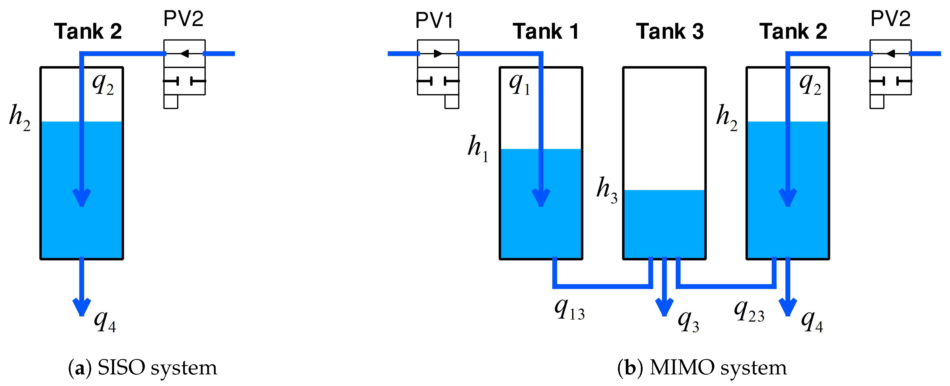
4. Problem Formulation from a Practical Point of View

4.1. Siso System Control

To control the water level in the SISO system presented in Figure 3, only the input data, $q_2$, and output data, $h_2$, of the system are required. The outlet $q_4$ is regarded as a disturbance. Hence, the nonlinear system (1) can be described as

$$h_2(k+1)=f\left(h_2\left(k\right),h_2(k-1),\dots ,h_2(k-n_y),q_2\left(k\right),q_2(k-1)\dots ,q_2(k-n_u)\right).$$

(37)

Accordingly, the CFDL and PFDL linearized models

$$h_2(k+1)=h_2\left(k\right)+{\varphi }_s\left(k\right)\Delta q_2\left(k\right)$$

(38)

and

$$h_2(k+1)=h_2\left(k\right)+\Phi \left(k\right)\Delta Q_L\left(k\right),$$

(39)

with

$$\begin{array}{cc}\hfill & Q_L\left(k\right)={[q_2\left(k\right),\dots ,q_2(k-L+1)]}^T,\hfill \\ \hfill & \Phi \left(k\right)=[{\varphi }_{s_1}\left(k\right),{\varphi }_{s_2}\left(k\right),\dots ,{\varphi }_{s_L}\left(k\right)],\hfill \end{array}$$

are obtained by applying the equivalent dynamic linearization techniques of Section 2.

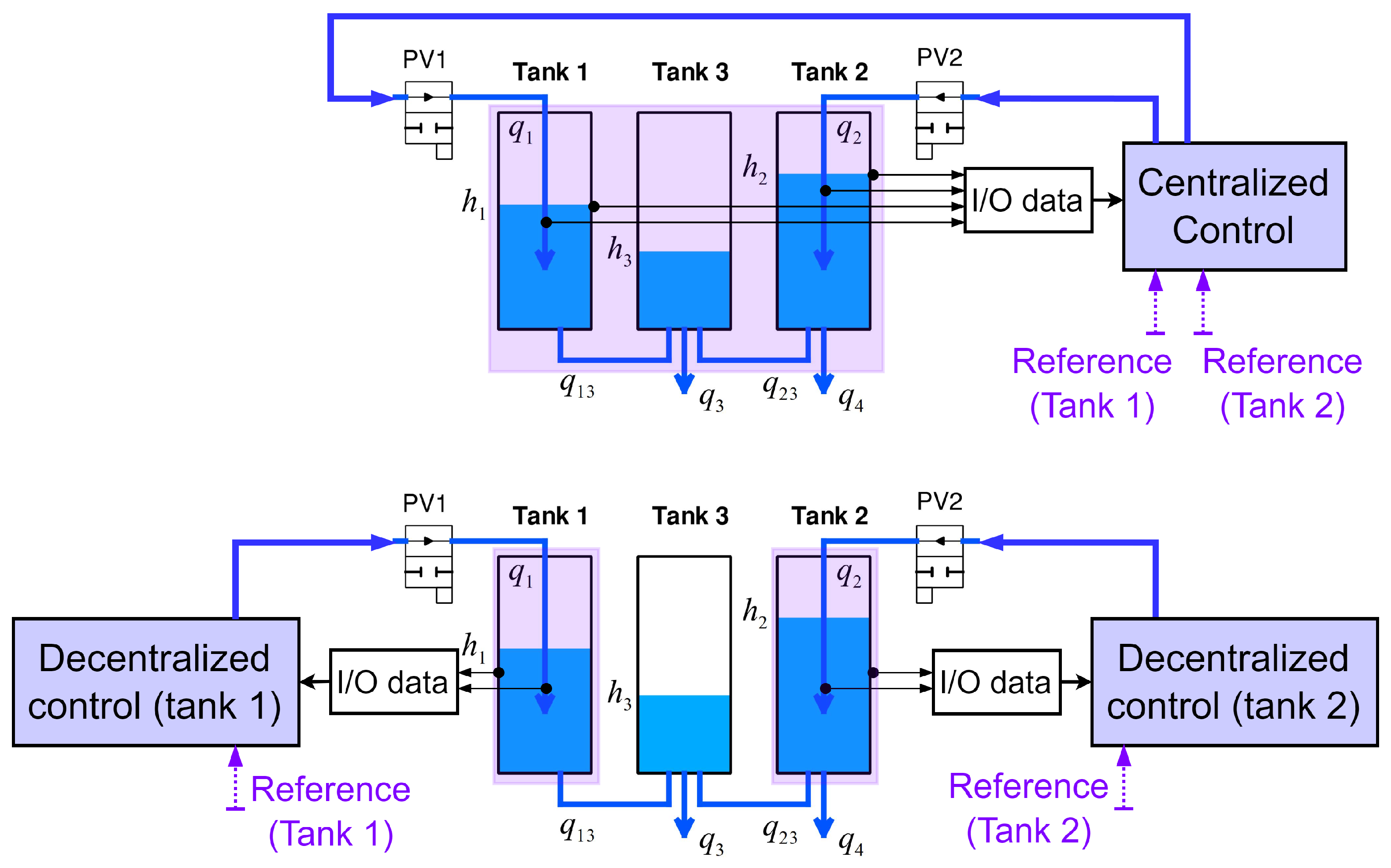
4.2. Multi-SISO System Control

Owing to the data-driven characteristics of MFAC, the outflows $q_{13}$ and $q_{23}$ in the MIMO 3TS depicted in Figure 3 can also be regarded as disturbances on tanks 1 and 2, respectively. The MIMO system is partitioned into two SISO subsystems (Figure 4), with $q_1$ and $q_2$ as water input flows and $h_1$ and $h_2$ as outputs. This consideration leads to a significant reduction in the PPD and PG matrix elements. This reduction is even more significant in MFACP, in which both estimation and prediction of the PPD are required. Therefore, the general formulation for the coupled multi-SISO system is

$$h_i(k+1)=f_i\left(h_i\left(k\right),\dots ,h_i(k-n_y),q_i\left(k\right),\dots ,q_i(k-n_u)\right),i=1,2.$$

(40)

Figure 4. Difference between centralized and decentralized MFAC, MMFAC, or MFAPC.

The linearized models based on CFDL and PFDL are

$$h_i(k+1)=h_i\left(k\right)+{\varphi }_{m_i}\left(k\right)\Delta q_i\left(k\right),i=1,2$$

(41)

and

$$h_i(k+1)=h_i\left(k\right)+{\Phi }_i\left(k\right)\Delta Q_{i_L}\left(k\right),i=1,2,$$

(42)

respectively, with

$$\begin{array}{cc}\hfill & Q_{i_L}\left(k\right)={[q_i\left(k\right),\dots ,q_i(k-L+1)]}^T,\hfill \\ \hfill & {\Phi }_i\left(k\right)=[{\varphi }_{m_{i,1}}\left(k\right),{\varphi }_{m_{i,2}}\left(k\right),\dots ,{\varphi }_{m_{i,L}}\left(k\right)].\hfill \end{array}$$

The test rig (Figure 2) is considered the main system controlled experimentally. The MFAC, MMFAC, and MFAPC controllers are implemented on the SISO system based on the linearized models in (38) and (39) and on a multi-SISO 3TS based on (41) and (42).

5. Experimental Results

5.1. Metric for Parameter Tuning and Performance Comparison

The efficiency of the controllers is evaluated based on finding a compromise between the output error and the energy consumed by the controller developed in [27]. Graphically, this criterion is an illustration of the Integral Squared Errors (ISEs) versus the Integral Squared Input (ISI)—representing the energy utilized by the controller as

$$\mathrm{ISE}\mathrm{vs}.\mathrm{ISI}=\left[{\int }_0^T\epsilon {\left(t\right)}^{2}dt,{\int }_0^{T}u{\left(t\right)}^{2}dt\right].$$

(43)

After repeating the experiment with various parameters for each controller, the control performances are compared according to (43). The controller with lower ISE and ISI values is considered to deliver better performance.

Proper tuning of parameters for MFAC is essential, as inappropriate parameters can have a negative impact on the control performance [29]. Parameter adjustment can be conducted through variety of techniques, such as using neural networks [29], reinforcement learning [30], or VRFT [31]. Determining the optimal parameters for the proposed controllers, leading to their best performance, can also be achieved using (43). In this process, the reference for tank 2 is set to 25 cm for a duration of 60 seconds, and the experiment is repeated with a systematic change in feasible values for the design parameters such as $\rho$, $\lambda$, $N_m$, s, and L. Consequently, the results are captured and compared using (43); the finally selected values of these design parameters are given in Table 2. The initial values $\varphi \left(1\right),{\varphi }_1\left(1\right),\dots ,{\varphi }_L\left(1\right)=0.1$ and design parameters $\eta =1$ and $\mu =1$ are considered for all the approaches.

Table 2. Parameters of the controllers.

Controller	Color	Parameters
		$\mathit{\rho }$	$\mathit{\lambda }$	${\mathit{N}}_{\mathit{m}}$	$\mathit{s}$	$\mathit{L}$
MFAC-CFDL		0.9	1	-	-	-
MFAC-PFDL		0.9	1	-	-	10
MMFAC-CFDL		0.9	1	20	0.1	-
MMFAC-PFDL		0.1	1	20	0.1	10
MFAPC-CFDL		0.9	1	-	-	-

For the MFAPC approach, additionally, an output horizon of $N=20$ and an input horizon of $N_u=1$ are chosen. By having $n_p=2$, the initial values ${\theta }_1\left(1\right)=0.5$ and ${\theta }_2\left(2\right)=0.1$, in addition to $\delta =1$, are considered. If the control horizon $N_u$ = 1 and the reference for the SISO partition is assumed to be constant for the whole parameter-tuning experiment, the predictive control $u\left(k\right)$ (34) becomes

$$u\left(k\right)=u(k-1)+\rho \varphi \left(k\right){\displaystyle \frac{\frac{1}{N}(h_2^{*}(k+1)-h_2\left(k\right))}{\lambda /N+{|\varphi \left(k\right)|}^2}}.$$

(44)

According to ([3], Remark 6.1), (44) is insensitive to the parameter $\lambda$ due to the division by N. Additionally, to see how prediction features in Section 2.4 affect the performance of the conventional MFAC-CFDL approach, $\rho =0.9$ is selected.

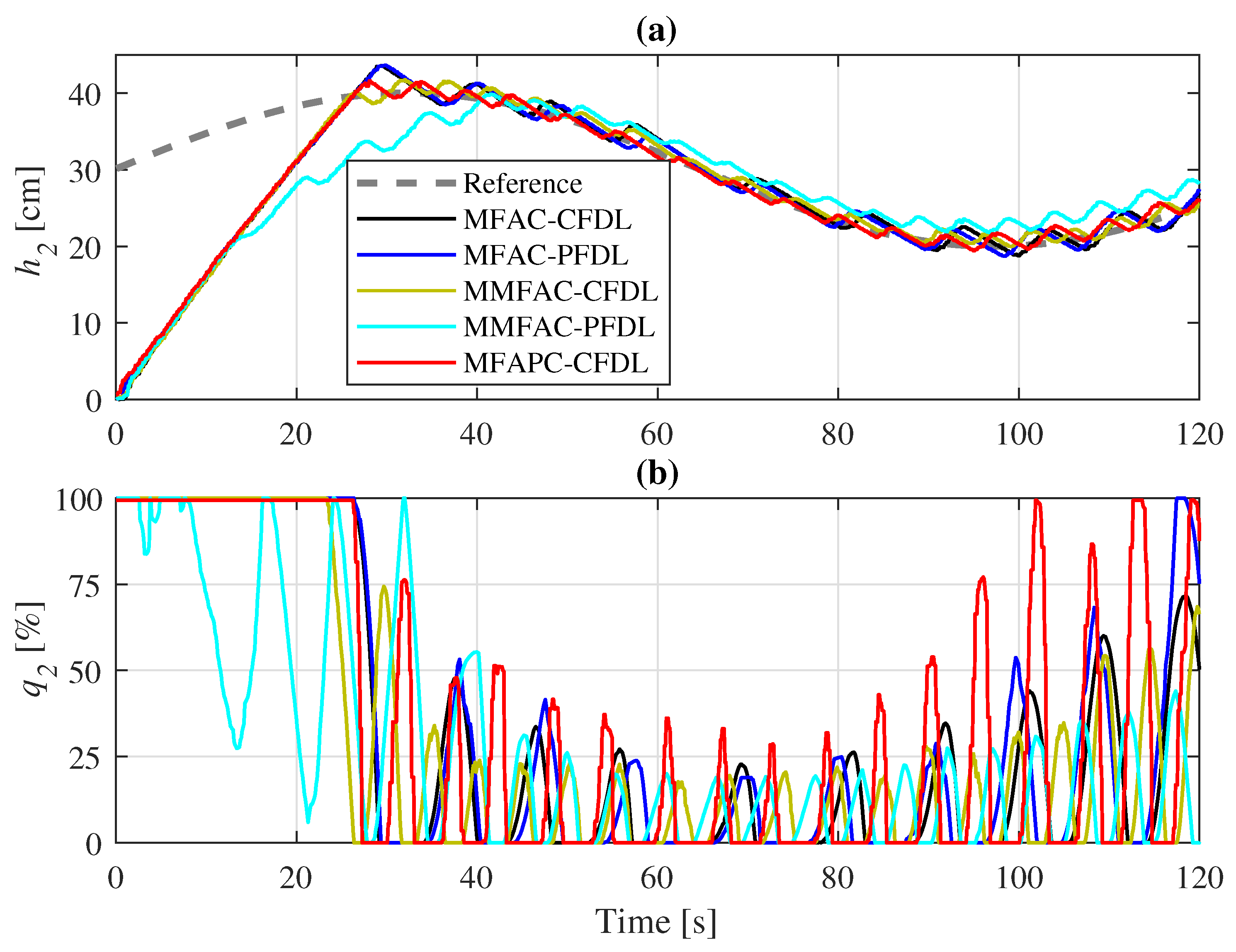
5.2. Comparison of Approaches for the Considered SISO System

The results of the applied controllers on tank 2 as an SISO system are presented. The constant reference of the system to be controlled changes according to

$$h_2^{*}\left(t\right)=\left\{\begin{array}{c}25\left[\mathrm{cm}\right]t\le 40\left[\mathrm{s}\right]\hfill \\ 40\left[\mathrm{cm}\right]40\left[\mathrm{s}\right]<t\le 80\left[\mathrm{s}\right]\hfill \\ 30\left[\mathrm{cm}\right]80\left[\mathrm{s}\right]<t\le 120\left[\mathrm{s}\right]\hfill \end{array}\right.$$

(45)

for the purpose of adaptability investigation. From Figure 5, it can be concluded that all controllers successfully track the reference trajectory. The predictive behavior of the MFAPC-CFDL approach is noticeable at $t=40$ [s]. Specifically, when considering $N=20$ and a sample time of 100 [ms], the MFAPC-CFDL integrates information from the desired reference for the next 2 [s], leading to an advanced increase in input flow when the desired reference is about to increase at $t=40$ [s].

Figure 5. Performanceof the controllers on the SISO system with constant reference having abrupt changes: (a) water level control and (b) input flow.

According to Figure 6, it becomes evident that the MFAPC-CFDL approach yields a better result in terms of cumulative ISE. Additionally, it can be confirmed from Figure 6 that the tracking performance of conventional MFAC can be improved by including predictive features. However, the MMFAC-CFDL and MMFAC-PFDL approaches still perform better in terms of energy consumption.

Figure 6. Performance evaluation of the controllers on the SISO system with constant reference having abrupt changes: (a) cumulative ISE, (b) cumulative ISI, and (c) performance evaluation.

The performance of the controllers is further evaluated when the SISO system has a time-varying reference. In Figure 7, the proposed controllers successfully follow the desired path, except for the MMFAC-PFDL controller, which does not exhibit proper energy consumption when the desired path varies over time. It is expected that the MFAPC controller will track the time-varying reference better as it updates the prediction horizon of $N=20$ with varying values of the reference, keeping the actual water level closer to the desired level (Figure 8). However, this improvement comes at the cost of investing more input energy, as can be concluded from the performance evaluation in Figure 8.

Figure 7. Performance of the controllers on the SISO system with time-varying reference: (a) reference control and (b) input flow.

Figure 8. Performanceevaluation of the controllers on the SISO system with time-varying reference: (a) cumulative ISE, (b) cumulative ISI, and (c) performance evaluation.

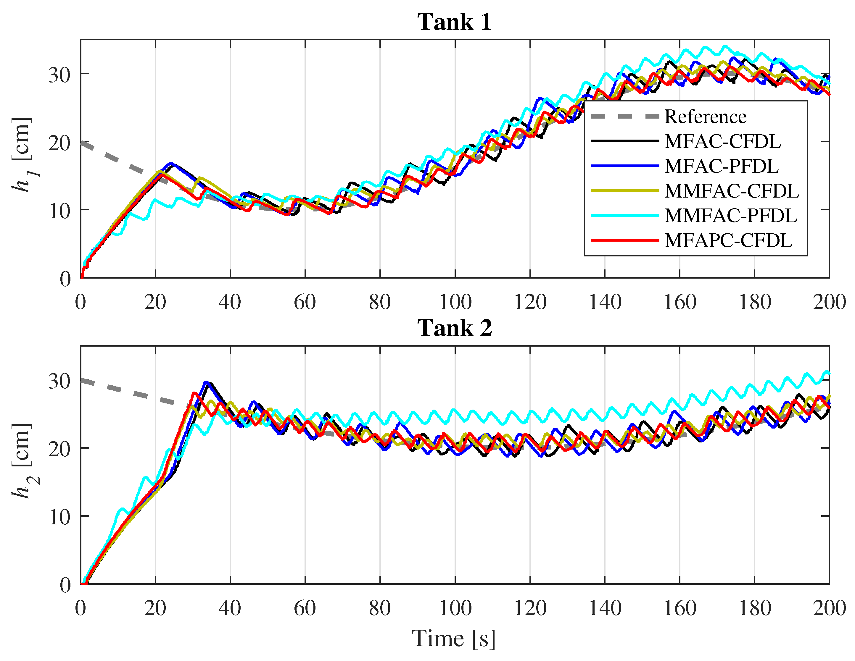
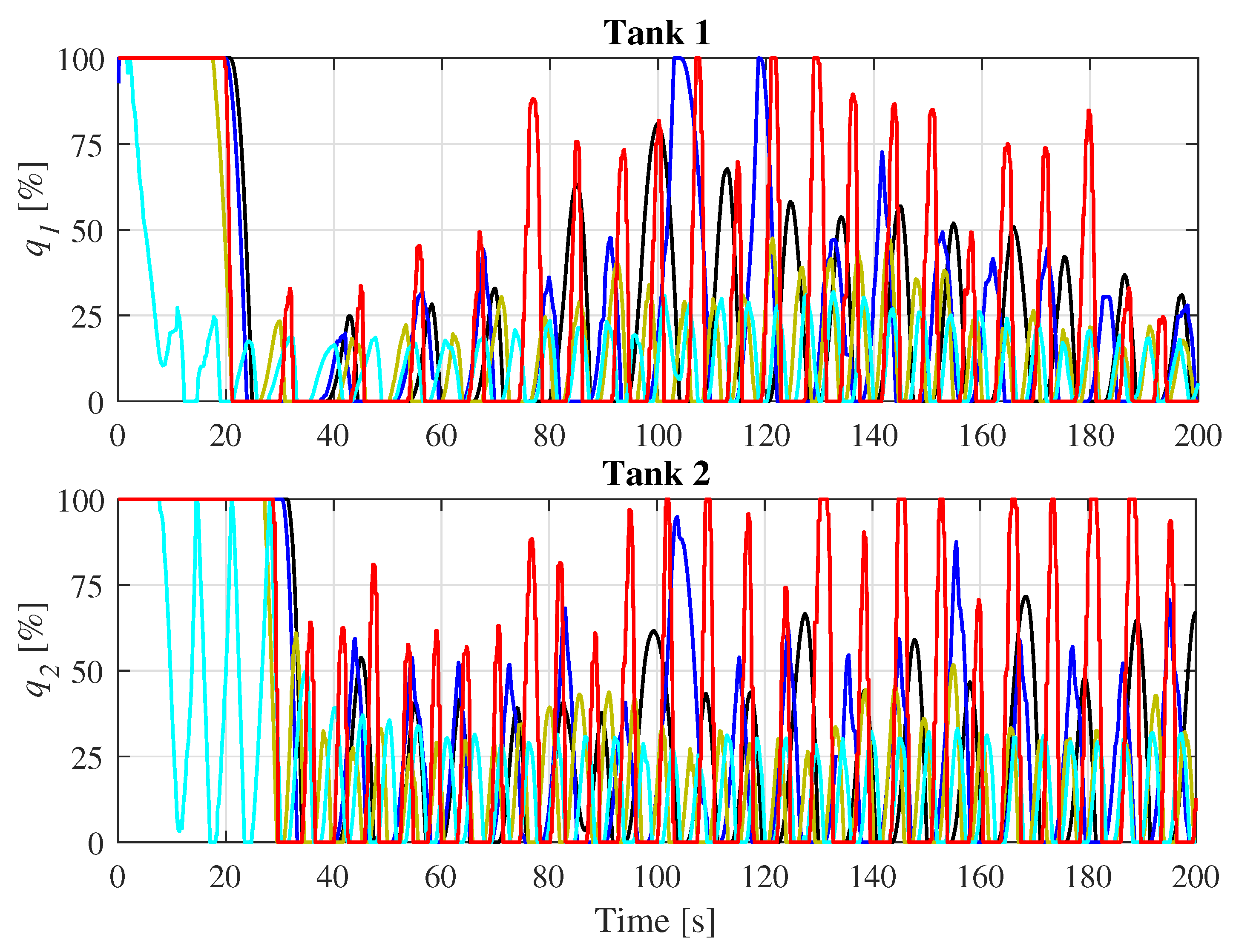
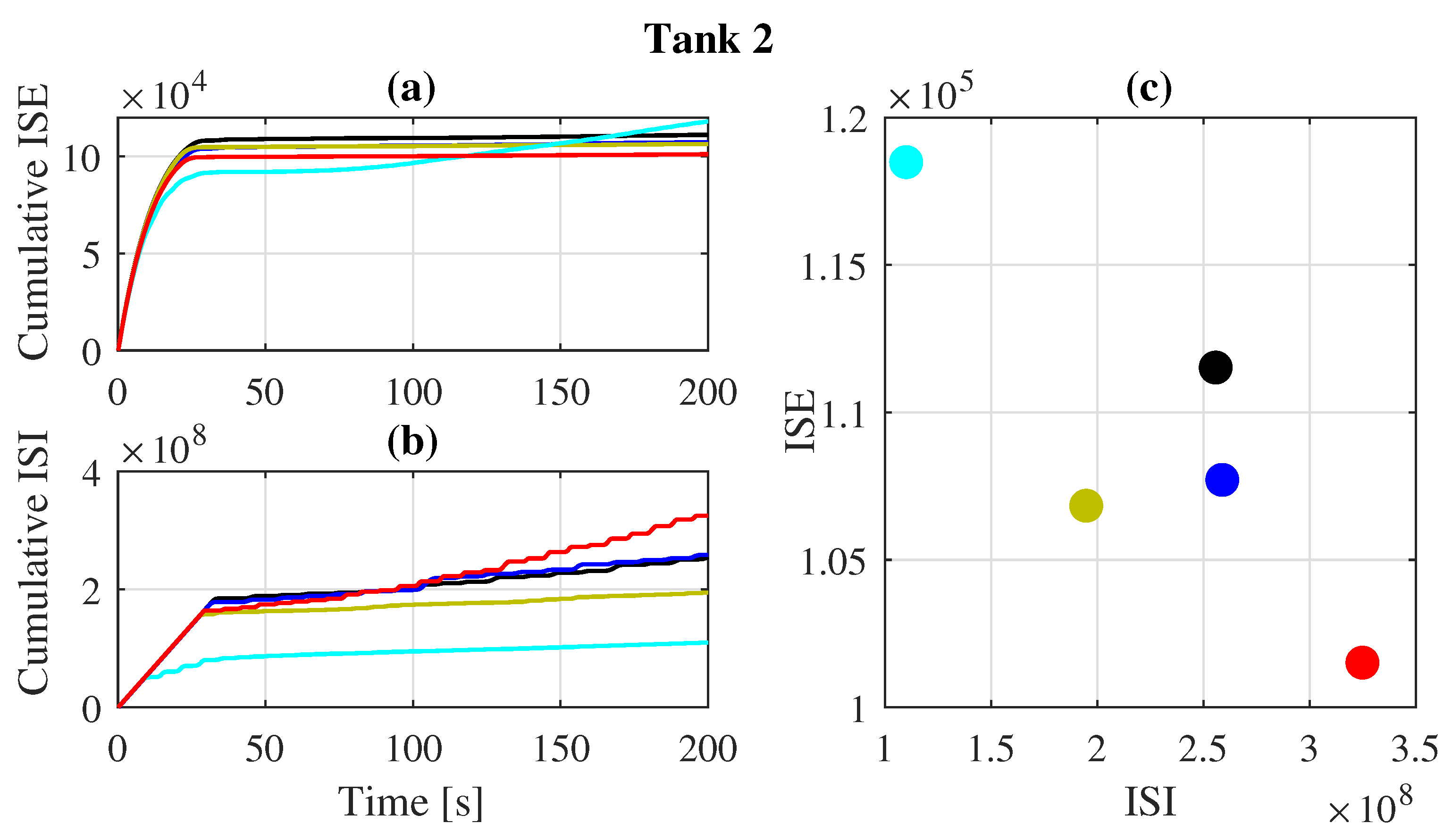
5.3. Comparison of Approaches for Multi-SISO System

In this section, the three-tank MIMO system is considered as an interconnection of SISO subsystems. The controllers are applied to each subsystem and work in parallel over a time span of 200 [s] to track a path that varies slowly between 10 [cm] and 30 [cm] in tank 1 and between 20 [cm] and 30 [cm] in tank 2. It can be seen from Figure 9 that the controllers’ performance in tracking the desired levels in both tanks is acceptable, except for MMFAC-PFDL, which cannot follow the desired levels. This is clearly shown in Figure 10, where the inputs of the controllers are compared over the whole experiment.

Figure 9. Tracking performance of the controllers on the multi-SISO 3TS with time-varying reference.

Figure 10. Control input flow on the multi-SISO 3TS with time-varying reference.

Figure 11 and Figure 12 provide information on changes in ISE and ISI for each tank throughout the experiment. MFAPC still demonstrates superior tracking performance for tank 2 compared to the other controllers. Additionally, as no direct outlet is considered for tank 1, there is less disturbance, resulting in the ISE values achieved for tank 1 being relatively close. It is also important to note that MFAPC consumes more energy due to its method of processing future information. The ISE-ISI graph further confirms that the use of MFAPC on each subsystem leads to relatively better tracking results than MFAC and MMFAC.

Figure 11. Performance evaluation of the controllers on decoupled tank 1 with time-varying reference: (a) cumulative ISE, (b) cumulative ISI, and (c) performance evaluation.

Figure 12. Performance evaluation of the controllers on decoupled tank 2 with time-varying reference: (a) cumulative ISE, (b) cumulative ISI, and (c) performance evaluation.

6. Summary and Conclusions

In this contribution, the reference tracking of an MIMO nonlinear system is experimentally conducted using various MFAC approaches, including conventional MFAC-CFDL/-PFDL, modified MFAC (MMFAC-CFDL/-PFDL), and a predictive approach (MFAPC-CFDL). The performance of the applied approaches is compared using the ISE-ISI criterion, cumulative ISE, and cumulative ISI. The experimental device is a nonlinearly coupled three-tank system. The novel approach in this contribution entails treating the influences of these nonlinear couplings as disturbances when applying the model-free adaptive controllers, which leads to simplification of the control algorithms in terms of there being fewer parameters to be tuned when separately applied to multiple SISO partitions of the whole MIMO system. The findings indicate that multi-SISO reference tracking is experimentally realizable due to the nature of the applied model-free adaptive controllers, while the design of a centralized MIMO control would be prohibitive. Furthermore, the results show that including predictive features in conventional MFAC-CFDL can lead to better reference tracking, especially with slowly time-varying references. On the other hand, MMFAC-CFDL/-PFDL results in reduced energy consumption.

References

- Ioannou, P.; Fidan, B. Adaptive Control Tutorial; SIAM: Philadelphia, PA, USA, 2006. [Google Scholar]
- Bakhshande, F.; Söffker, D. Robust control approach for a hydraulic differential cylinder system using a Proportional-Integral-Observer-based backstepping control. In Proceedings of the 2017 American control conference (ACC), Seattle, WA, USA, 24–26 May 2017; pp. 3102–3107. [Google Scholar]
- Hou, Z.; Jin, S. Model Free Adaptive Control; CRC Press: Boca Raton, FL, USA, 2013. [Google Scholar]
- Salighe, S.; Söffker, D. On the PID-structured model-free adaptive control: A comparison of different approaches. In Proceedings of the 2024 European Control Conference (ECC), Stockholm, Sweden, 25–28 June 2024; pp. 1309–1314. [Google Scholar]
- Hou, Z.; Jin, S. Data-driven model-free adaptive control for a class of MIMO nonlinear discrete-time systems. IEEE Trans. Neural Netw. 2011, 22, 2173–2188. [Google Scholar] [PubMed]
- Hou, Z.; Jin, S. A novel data-driven control approach for a class of discrete-time nonlinear systems. IEEE Trans. Control. Syst. Technol. 2010, 19, 1549–1558. [Google Scholar] [CrossRef]
- Hou, Z.; Zhu, Y. Controller-dynamic-linearization-based model free adaptive control for discrete-time nonlinear systems. IEEE Trans. Ind. Inform. 2013, 9, 2301–2309. [Google Scholar] [CrossRef]
- Pham, H.A.; Söffker, D. Modified Model-Free Adaptive Control using Compact-Form Dynamic Linearization Technique. IFAC-PapersOnLine 2020, 53, 3940–3945. [Google Scholar] [CrossRef]
- Li, J.; Wang, S.; Li, Y. A model-free adaptive controller with tracking error differential for collective pitching of wind turbines. Renew. Energy 2020, 161, 435–447. [Google Scholar] [CrossRef]
- Xiong, H.; Liao, Y.; Chu, X. Improved model free adaptive control for winding system. In Proceedings of the 2018 IEEE 7th Data Driven Control and Learning Systems Conference (DDCLS), Enshi, China, 25–27 May 2018; pp. 396–401. [Google Scholar]
- Xiong, S.; Hou, Z. Model-free adaptive control for unknown MIMO nonaffine nonlinear discrete-time systems with experimental validation. IEEE Trans. Neural Netw. Learn. Syst. 2020, 33, 1727–1739. [Google Scholar] [CrossRef] [PubMed]
- Roman, R.C.; Radac, M.B.; Precup, R.E. Data-driven model-free adaptive control of twin rotor aerodynamic systems. In Proceedings of the 9th IEEE International Symposium on Applied Computational Intelligence and Informatics (SACI), Timisoara, Romania, 15–17 May 2014; pp. 25–30. [Google Scholar]
- Zen, Z.; Cao, R.; Hou, Z. MIMO model free adaptive control of two degree of freedom manipulator. In Proceedings of the 2018 IEEE 7th Data Driven Control and Learning Systems Conference (DDCLS), Enshi, China, 25–27 May 2018; pp. 693–697. [Google Scholar]
- Li, Z.; Jin, S.; Xu, C.; Li, J. Model-free adaptive predictive control for an urban road traffic network via perimeter control. IEEE Access 2019, 7, 172489–172495. [Google Scholar] [CrossRef]
- Guo, Y.; Hou, Z.; Liu, S.; Jin, S. Data-driven model-free adaptive predictive control for a class of MIMO nonlinear discrete-time systems with stability analysis. IEEE Access 2019, 7, 102852–102866. [Google Scholar] [CrossRef]
- Hou, Z.; Liu, S.; Tian, T. Lazy-learning-based data-driven model-free adaptive predictive control for a class of discrete-time nonlinear systems. IEEE Trans. Neural Netw. Learn. Syst. 2016, 28, 1914–1928. [Google Scholar] [CrossRef]
- Wang, Y.; Hou, M. Model-free adaptive integral terminal sliding mode predictive control for a class of discrete-time nonlinear systems. ISA Trans. 2019, 93, 209–217. [Google Scholar] [CrossRef] [PubMed]
- Ji, H.; Wei, Y.; Fan, L.; Liu, S.; Wang, Y.; Wang, L. Disturbance-d Model-Free Adaptive Prediction Control for Discrete-Time Nonlinear Systems with Time Delay. Symmetry 2021, 13, 2128. [Google Scholar] [CrossRef]
- Tan, H.; Wang, Y.; Wu, M.; Huang, Z.; Miao, Z. Distributed group coordination of multiagent systems in cloud computing systems using a model-free adaptive predictive control strategy. IEEE Trans. Neural Netw. Learn. Syst. 2021, 33, 3461–3473. [Google Scholar] [CrossRef] [PubMed]
- Wang, S.; Li, J.; Hou, Z.; Meng, Q.; Li, M. Composite Model-free Adaptive Predictive Control for Wind Power Generation Based on Full Wind Speed. CSEE J. Power Energy Syst. 2020, 8, 1659–1669. [Google Scholar]
- Li, D.; De Schutter, B. Distributed model-free adaptive predictive control for urban traffic networks. IEEE Trans. Control. Syst. Technol. 2021, 30, 180–192. [Google Scholar] [CrossRef]
- Antonelli, G. Interconnected dynamic systems: An overview on distributed control. IEEE Control. Syst. Mag. 2013, 33, 76–88. [Google Scholar]
- Ioannou, P.; Kokotovic, P. Decentralized adaptive control of interconnected systems with reduced-order models. Automatica 1985, 21, 401–412. [Google Scholar] [CrossRef]
- Zhu, Y.; Qian, F.; Hou, Z.; Jin, S. Data-driven model free adaptive control for a class of interconnected systems. In Proceedings of the 2015 10th Asian Control Conference (ASCC), Sabah, Malaysia, 31 May–3 June 2015; pp. 1–6. [Google Scholar]
- Qi, J.; Cao, R.; Hou, Z.; Zhou, H. The model-free adaptive control for complex connected systems in the H-type motion platform. In Proceedings of the 2017 6th Data Driven Control and Learning Systems (DDCLS), Chongqing, China, 26–27 May 2017; pp. 129–134. [Google Scholar]
- Li, Y.; Hou, Z.; Hao, J. Decentralized model-free adaptive control for signalized intersections network. IFAC Proc. Vol. 2013, 46, 88–93. [Google Scholar] [CrossRef]
- Liu, Y.; Söffker, D. Improvement of optimal high-gain PI-observer design. In Proceedings of the 2009 European Control Conference (ECC), Budapest, Hungary, 23–26 August 2009; pp. 4564–4569. [Google Scholar]
- Madadi, E.; Dong, Y.; Söffker, D. Comparison of different model-free control methods concerning real-time benchmark. J. Dyn. Syst. Meas. Control. 2018, 140, 121014. [Google Scholar] [CrossRef]
- Yang, Y.; Chen, C.; Lu, J. Parameter self-tuning of SISO compact-form model-free adaptive controller based on long short-term memory neural network. IEEE Access 2020, 8, 151926–151937. [Google Scholar] [CrossRef]
- Liu, S.; Jia, X.; Ji, H.; Fan, L. Parameter optimization design of MFAC based on Reinforcement Learning. In Proceedings of the 2023 IEEE 12th Data Driven Control and Learning Systems Conference (DDCLS), Xiangtan, China, 12–14 May 2023; pp. 1036–1043. [Google Scholar]
- Roman, R.C.; Radac, M.B.; Precup, R.E.; Petriu, E.M. Data-driven model-free adaptive control tuned by virtual reference feedback tuning. Acta Polytech. Hung. 2016, 13, 83–96. [Google Scholar]
Disclaimer/Publisher’s Note: The statements, opinions and data contained in all publications are solely those of the individual author(s) and contributor(s) and not of MDPI and/or the editor(s). MDPI and/or the editor(s) disclaim responsibility for any injury to people or property resulting from any ideas, methods, instructions or products referred to in the content. |
© 2024 by the authors. Licensee MDPI, Basel, Switzerland. This article is an open access article distributed under the terms and conditions of the Creative Commons Attribution (CC BY) license (https://creativecommons.org/licenses/by/4.0/).