Reliability Analysis of an IoT-Enabled Street-Side Plant Bed Protection and Monitoring System in Residential Areas

Abstract

Unauthorized plucking of flowers, fruits, and vegetables from residential plant beds is a recurring concern in urban and semi-urban household, causing damage to gardening resources, economic loss and inconvenience to sustainable gardening. To address this issue, the present study proposes an IoT-enabled Smart Residential Plant Bed Protection System (SRPBPS), which is the integration of motion sensors, plant disturbance sensors, a video monitoring unit, a microcontroller, a communication module, and an alarm mechanism for real-time intrusion detection and monitoring. The behaviour of the proposed system is analyzed using a continuous-time Markov modelling approach by considering various operational and failed states of system components. Important reliability measures, including system reliability, mean time to system failure (MTTF), and the expected number of failures over time, are evaluated analytically. In addition, sensitivity analysis of reliability and MTTF are carried out to identify the critical components influencing overall system performance. The obtained results provide useful insights into component-level impact on system effectiveness and support reliability-oriented design enhancement. The proposed framework contributes toward the development of intelligent, secure, and sustainable residential plant bed protection systems for modern residential environments.

1. Introduction

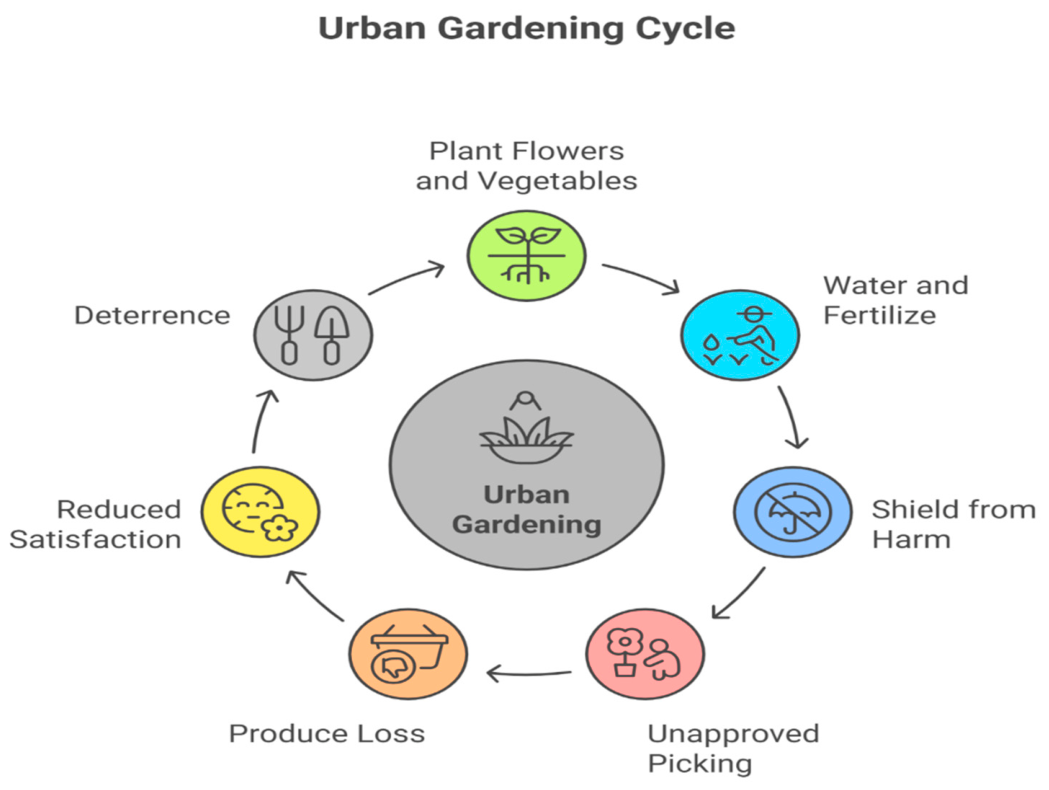
With the spread of urbanization, more and more urban households are cultivating flowers, fruits and vegetables in the plant beds, called kyares, that are set outside their homes along the streets and next to boundary walls. These small-scale fields provide additional food for families, environmental balance and beauty. Many of the residents spend time, energy and money caring for these plant beds—watering, fertilizing, and protecting them from damaging environmental factors. This micro-gardening also contributes to the urban greenery and eco-friendly actions of urban society living in very populated residential areas. Yet, the unauthorized picking of flowers, fruits and vegetables by passers-by is not an uncommon problem encountered by many of the households. The location of these plant beds, however, is in open areas outside the house and is readily available to all the neighbours and passers-by. As a result of this, there is often an issue of people plucking flowers or vegetables without permission, sometimes for fun and sometimes by accident. Loss of produce is common, and the satisfaction of household members who care for these plants is reduced because of this behaviour. This problem eventually contributes to discouraging people from maintaining their outside plant beds, thereby negatively affecting urban gardening techniques. This is indicated in Figure 1.

The problem is compounded by poor monitoring systems, as well as produce loss. The majority of households do not have time to regularly check the outdoor plant beds. In recent years, the solution of problems related to the Internet of Things (IoT)-based systems and the smart monitoring technologies in the field of crop protection and agriculture have become possible again. Sensors, cameras, and communication modules can be used in intelligent monitoring systems to detect disruptions and notify users immediately. Protection of home plant beds in cities has received little research attention, particularly when viewed from a reliability engineering perspective, although there are many smart monitoring devices in the market. Most existing studies are dedicated to technologies related to crop security, wildlife entry detection or widespread agricultural surveillance. However, there has not been much discussion of the issue of illegal plucking of fruits, vegetables and flowers from plant beds in the scholarly literature. Operational performance and reliability of these protection systems need to be comprehensively assessed to ensure their long-term successful operation. To fill this gap, the present study proposes a Smart Residential Plant Bed Protection System which can detect the disturbances of the plant bed and alert the homeowners in case of unapproved plant bed plucking. The proposed system includes motion sensors, plant disturbance sensors, camera modules, microcontrollers, communication modules, and alarm systems. To assess the performance of the system, reliable modelling of the system is required, as the dependability of these interconnected components is critical to the correct functioning of the system.

In this study, the processes involved in the operation and failure of the proposed system are modelled by Markov models. The Markov technique is useful for modelling stochastic transitions between different states of the system, which are caused by a failure or repair of one of the components [1,2,3]. The established model is used to calculate important reliability indices such as system reliability and mean time to first failure. These indices offer insightful information about the system’s reliability and assist in identifying crucial elements that have a major impact on the system’s overall performance. Therefore, this study’s main goal is to create a reliability model for a smart home plant bed protection system and assess its effectiveness using Markov processes. The outcomes of this research can be used to create more reliable monitoring methods to be used to protect plant beds for domestic use and to encourage more sustainable methods of urban gardening. The remaining parts of the paper are organized in this fashion. The literature review section is given in Section 2. In Section 3 the key definitions of reliability are given. In Section 4 a description of the system’s components is given. In Section 5 a mathematical formulation of the system is given. In Section 6 a performance analysis of the system is given. In Section 7 the results and discussion are given. In Section 8 the conclusion is given. In Section 9 future scopes are given.

Problem Statement

In urban areas, people are very fond of growing fruits, vegetables and flowers from household plant beds (kyaries) outside of homes. Passers-by from this road often pluck fruits, vegetables and flowers without the permission of the household owners, which ultimately discourages them to grow plants of various kinds outside their home. This practice has been prevalent for a long time without any effective proper technological solution available in the market. In order to identify and stop this unwanted act, the current study suggests a Smart Residential Plant Bed Protection System (SRPBPS). To monitor plant beds and warn the homeowner when suspicious activity takes place, the system incorporates motion sensors, plant disturbance sensors, a video module, a microcontroller unit, a communication module, and an alarm mechanism. This system helps the house owner protect their kyaries from the outsider.

2. Literature Review

The following section shows results from different researchers in relation to garden protection systems, smart surveillance technologies, and reliability analysis. Much work has been done on the design of strong and intelligent garden, farm and home protection systems. Since then, gardening has become an ever growing activity around the world, including at home in the family garden, which allows individuals to grow flowers, fruits and vegetables for aesthetic, nutritional and recreational uses. Nevertheless, there are some security issues like plant vandalism, stealing fruits and vegetables, and unauthorized entry that have become significant concerns. To solve the issues, various technological and non-technological solutions have been suggested, from fence systems to the use of the Internet of Things, as well as the use of sensors and alarms and systems for continuous observation. While these studies make important contributions, there is little literature on small-scale residential gardens, where theft by passer-by is a problem, and more work needs to be done on that setting. Hence, the need for a reliable, cost effective and efficient smart protection system with specific application for the protection of plant beds and home gardens is felt.

In the literature, fencing is regarded as one of the more initial and simple methods of farm and garden protection. Ref. [4] gathered field observations and documentation from all over Australia to examine the effects of barbed wire fencing on animals. The author undertook a case study in the Euroa region and analyzed data from a number of sources to identify species that are affected by fence entanglement. According to the study, at least 62 different animal species were discovered ensnared in barbed wire, with birds and gliders being the most impacted. The author also examined the reasons for entanglement, where it occurs and its trends, focusing on the harmful impact of this type of fencing on wildlife. Finally, the study suggested the use of a number of fencing methods to increase safety and reduce animal deaths. This study identified the protective effects of the fencing, but also demonstrated the environmental and ecological disadvantages of fencing. Turning this discussion to the effectiveness of fencing systems, Ref. [5] analyzed 54 papers on wildlife fencing in Africa and its contribution to mitigating HWC. The researchers looked at the cost, maintenance and effectiveness of different types of fences and found that electric fences are the most popular fences but their effectiveness is dependent on environmental conditions and proper maintenance. The study additionally discovered that while fencing decreases crop injury, it is not useful because many species may breach or bypass fences. Overall, both studies suggest that traditional fencing would be insufficient for the complete reliability and sustainability of a solution so intelligent monitoring and intrusion detection are required.

Ref. [6] compared the effects of virtual fencing on cow behaviour and welfare to that of electric tape fencing. Over the four-week period, the scientists tracked body weight, the level of cortisol metabolites in the animals’ feces, the amount of time the animals spent lying down, standing up, using the GPS, and how fast they learned to connect an electrical signal with an auditory signal. There was some variation in lying time, in individual rate of learning, but the results indicate that virtual fencing was as effective as electric tape fencing for containing cattle in specific areas with no measurable welfare side effects. This shift away from traditional fencing to virtual and intelligent fencing drives the increasing need for automated and sensor-based security solutions. Ref. [7] proposed a stochastic modelling approach using the Langevin equation to study mode coupling in multimode step-index plastic optical fibres (SI-POFs). Their work examined the random redistribution of optical power among propagation modes due to intrinsic fibre perturbations and assessed the steady-state power distribution through Monte Carlo simulations. This model demonstrated excellent agreement with experimental data and surpassed traditional deterministic methods in both accuracy and computational efficiency. The stochastic framework is valuable for evaluating signal degradation, modal dispersion, bandwidth performance, and reliability in optical communication and fibre-sensing systems.

As IoT and embedded technologies advanced, researchers slowly began to focus on smart home monitoring and automatic surveillance systems. Ref. [8] created a wireless multihop sensor network-based remote real-time monitoring and control management system for smart home appliances. The system was connected to a single chip microcontroller, Wi-Fi module (ESP8266, Espressif Systems, Shanghai, China) and cloud server through which indoor air quality, gas concentration, and the presence of people (human infrared activity) were monitored. They proposed a multi-sensor data fusion security method based on fuzzy logic reasoning and BP neural networks to detect abnormalities such as gas leakage, fire, and illegal intrusion. Experimental results showed that the system was able to achieve high detection accuracy with minimal false and missed alarms, thereby offering a reliable and practical solution for home security systems in smart homes. Similarly, Ref. [9] developed a real-time alarm system for home monitoring, which is based on both motion sensing and GSM technologies. The system included a GSM modem, a web camera to detect any activity, and FTP storage to send e-mails with photos attached. The method was built by using MATLAB (R2012a)(2.4.x/2.3.x)(2005) to support the motion detection, motion tracking and motion recognition. The results revealed that the motion detection system would automatically trigger SMS and email alerts, providing a cost-effective and flexible alternative to expensive commercial surveillance systems. It was evident from these studies, that motion sensing and communication technology can help to enhance the security and real-time response.

In order to develop smart surveillance systems, Keat and Wen [10] fabricated a smart interior home surveillance monitoring system using a passive infrared (PIR) motion sensor, a webcam and internet connection with a raspberry pi computer. The technology was designed to detect human movement, capture images of intruders, and send them to the homeowner in real time via email and SMS. It also automatically uploaded collected photos to Dropbox cloud storage for effective archiving and future verification and provided a live video stream. The object-oriented analysis and design (OOAD) methodology and Python (3.12.0) programming were used by the authors to implement the system. Testing results confirmed that the system was able to successfully gain motion detection, provide faster notifications and reduce storage space usage compared to the conventional CCTV system. Likewise, Dey et al. [11] had developed their home automation and security system by employing an Arduino Uno microcontroller and an Ethernet shield connected with a Wi-Fi router, which eventually resulted in an online real-time home automation and security system. The system offered a combination of security, automatic and manual operating modes, and was successfully able to offer intrusion detection, energy conservation and appliance control, and alarm initiation. These studies combined demonstrated the feasibility of low-cost embedded systems and monitoring technologies enabled by the IoT for home security applications. In order to detect Distributed Denial-of-Service (DDoS) assaults in smart microgrid communication infrastructures, Haxhismajli et al. [12] suggested an unsupervised CNN–LSTM-based anomaly detection system. Using only regular operational technology (OT) traffic, the authors created a dual-branch deep learning architecture that combines CNN for flow-based traffic feature extraction and LSTM for temporal network metric analysis. This architecture does not require labelled attack data. The framework outperformed autoencoder and isolation forest models in detection when tested against Modbus TCP, MQTT, and DNP3 protocol-specific DDoS attack scenarios. The suggested method can be successfully used to improve industrial communication networks and smart microgrids’ cybersecurity, dependability, and real-time monitoring.

As smart surveillance systems become increasingly complex, the need for reliability analysis has also increased in importance. The need for reliability analysis has also increased in importance as the smart surveillance systems become more complex. Reliability theory is of paramount importance when it comes to home security devices like intrusion detection systems, motion detectors, cameras, and alarm systems, as it could directly affect the safety of the person, and the safety of their home. Home security systems should be well-designed, prompt and effective in detecting unauthorized intrusions, yet not trigger false alarms or miss real threats. Reliability-wise, the failure rates of components like PIR sensors, Wi-Fi modules, cameras, and microcontroller affect the entire system’s performance, availability, and maintenance needs. Therefore, reliability theory provides a systematic solution for the assessment, prediction and enhancement of the dependable operation of such systems.

In this direction Ram [13] performed a comprehensive study on dependability theory methods and the application of these methods in engineering and physical sciences. The author analyzed fourteen key approaches to reliability, such as Bayesian methods, neural networks, optimization, distributed systems, risk analysis and statistical approaches. The study pointed to the accelerated development and wide range of applicability of reliability theory in different engineering fields. Based on these theoretical bases, Maihulla et al. [14], studied the availability and reliability of a two series-parallel system of components using stochastic theory, Laplace transforms and Gumbel-Hougaard copula repair modelling. The results showed that the performance of the system decreases over time, but it can be improved significantly when proper repair policies are applied. Likewise, Musa et al. [15] used Markov chain modelling and Chapman–Kolmogorov equations to analyze a centrifugal water pumping system using RAMD analysis. Their results revealed that there is a direct link between repair rates, component reliability and overall system performance. All these studies confirmed that the stochastic and the Markov methods were effective for reliability analysis of complicated engineering systems.

In addition to the traditional reliability modelling, researchers have also introduced optimization approaches into reliability engineering. Refs. [16,17] used reliability theory and Markov state-based modelling techniques to create reliability analysis of automated systems like Seabin water cleaning system and waste sorting robotic arm system (WSRAS). The reliability indices, such as reliability, availability, MTTF and sensitivity analysis were derived using the Chapman–Kolmogorov equations and Laplace transforms. The critical components that, if they failed, would have the greatest impact on the overall system performance were identified through sensitivity analysis. The significance of weak subsystems identification for enhancing the overall reliability and maintenance planning was highlighted in these studies.

There has also been a lot of research interest in the optimization of system reliability. To address a multi-objective reliability optimization problem of a space capsule life-support system under fuzzy constraints, a non-dominated sorting genetic algorithm (NSGA-II) was used by Kishor et al. [18]. They managed to come up with Pareto-optimal solutions that resulted in both cost and reliability being minimized. In a similar fashion, Sharma and Kumar [19] investigated the reliability of a two-unit hot standby system with WEID and showed that the Bayesian estimators outperformed the maximum likelihood estimators when informative priors were assumed. In these investigations, the role of advanced mathematical and probabilistic approaches for reliability optimization and performance evaluation was further consolidated.

Also, Ref. [20] merged fault tree analysis, rule-based reasoning and Bayesian optimization for fault detection in heavy CNC machine tools. The study integrated fault diagnosis and probabilistic reasoning to enhance the accuracy of fault detection and efficiency of operation under uncertainty. The present work effectively illustrates intelligent fault diagnosis and reliability analysis integration to create robust and reliable automatic systems.

Based on the above literature review, it could be concluded that there has been a significant amount of work performed in fencing systems, smart surveillance technologies, engineering system monitoring through IoT, and reliability analysis of engineering systems. Manual supervision, traditional fencing, CCTV surveillance, and standalone alarm systems are the mainstays of current home plant protection options. These methods typically do not take system resilience under component failures into account and offer limited real-time responsiveness. The suggested IoT-enabled SRPBPS, on the other hand, combines sensing, monitoring, communication, and alarm mechanisms into a single smart framework that can identify intrusions in real time. Additionally, in contrast to current technologies, the suggested study uses a Markov-based reliability analysis to assess system performance, pinpoint crucial elements, and promote reliability-centred design enhancements for sustainable residential gardening applications.

The proposed SRPBPS is specifically targeted at flowers, fruits, and vegetables in household plant beds (kyarie) outside the house. The novelty of the paper is that the system features a combination of intelligent sensing, monitoring and alarm components to provide a solution to both detect unauthorized use and to enhance security for the residential garden. Reliability analysis is important for assessing the reliability of the system under various operating conditions because the effectiveness of such a system heavily relies upon the reliable performance of the elements of the system. To this end, some basic terms and concepts of reliability engineering used in the current study are introduced in the following section.

3. Key Definitions

The key definitions of reliability theory are presented in this section.

3.1. Reliability Function

Reliability is defined as the probability that a system (component) will function over some time period $t$ [3]. To express this relationship mathematically we define the continuous random variable $T\ge 0$ to be the time to failure of the system (component). Then reliability can be expressed as given below.

$$R\left(t\right)=\mathit{Pr}(T\ge t)$$

where $R\left(t\right)\ge 0$, $R\left(0\right)=1$ and $\underset{t\to \infty }{lim}R(t)=0$. For a given value of $t$, $R\left(t\right)$ is the probability that the time to failure is greater than or equal to t.

3.2. Mean Time to Failure (MTTF)

It is one of the most critical measures of system performance, which gives detailed insight into a system’s failure time. Mathematically it is defined as:

$$\begin{array}{cc}\hfill \mathrm{MTTF} = E\left(T\right)& ={\int }_0^{\infty }t.f\left(t\right)dt\hfill \\ & ={\int }_0^{\infty }R\left(t\right)dt\end{array}$$

3.3. Failure Rate

According to reliability theory, a system’s or component’s failure rate is a measure of how frequently it is likely to fail over time, assuming that it is currently operational. The failure rate of a component is denoted by $\lambda (t)$.

3.4. Repair Rate

In reliability theory, repair rate refers to the speed at which a malfunctioning system or component is put back in working order. The repair rate is denoted by $\mu \left(t\right)$.

3.5. Perfect Working State

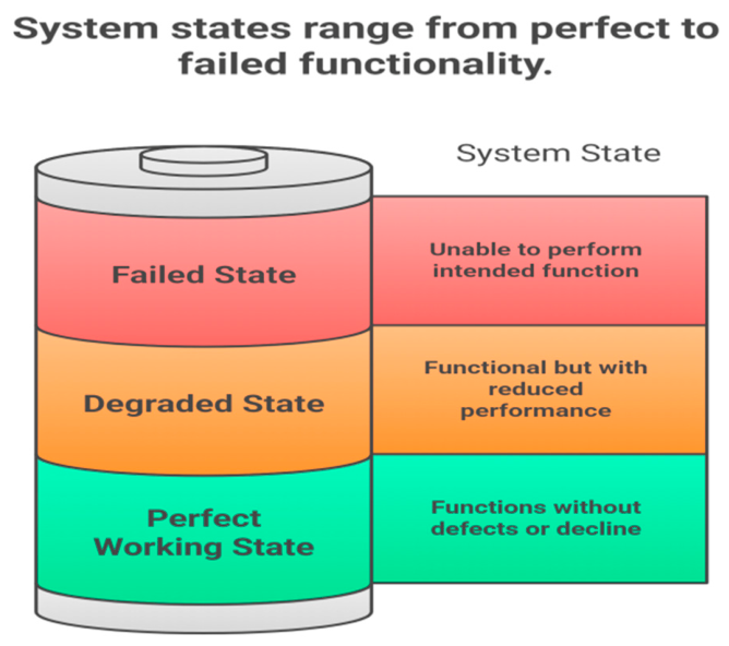
A system is said to be in its perfect functional state when it functions flawlessly, free from defects, damage, or performance decline.

3.6. Degraded State

A system in a degraded state is one that is still functional but exhibits diminished performance as a result of wear or partial malfunctions.

3.7. Failed State

A system is said to be in a failed state when it is unable to carry out its intended function.

Figure 2 depicts the perfect working state, the degraded state, and the failed state of the system.

4. Description of System Components

The description of the system’s components is presented below:

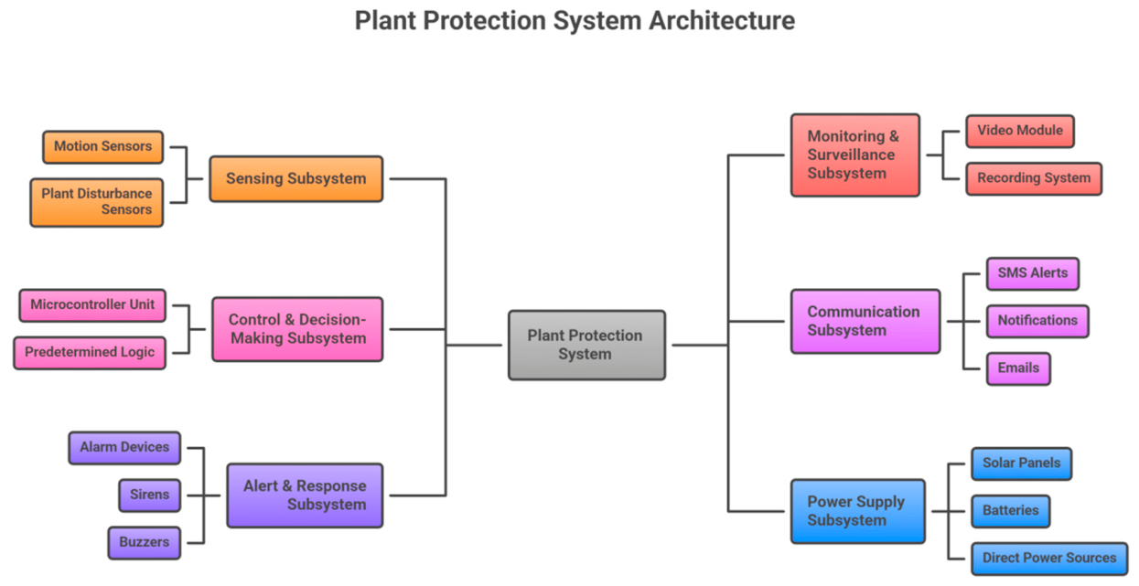
• Sensing Subsystem: Any physical activity near the plant bed must be detected by the sensing subsystem. It is made up of motion sensors and plant disturbance sensors that keep an eye on the environment at all times. While disturbance sensors detect direct involvement, such as picking or harming plants, motion sensors detect the presence of people or animals. When anomalous behaviour takes place, this component generates signals to serve as the first line of defence.
• Monitoring and Surveillance Subsystem: This subsystem uses the video module (camera) to offer visual monitoring of the protected area in real time. When any action is detected by the sensing subsystem, it becomes active. The recorded photos or videos aid in confirming the authenticity of the identified event. It also acts as a recording system for proof or future reference.
• Control and Decision-Making Subsystem: This is the system’s central intelligence and is controlled by the microcontroller unit (MCU). After gathering input signals from the sensor subsystem, it processes them following a preprogrammed logic. Once the activity is determined to be suspicious or normal, it activates other subsystems such as communication and alarm. It ensures the correct coordination of all the elements of the system.
• Communication Subsystem: The communication subsystem processes the information that is communicated from the system to the homeowner. It alerts you in real time through SMS, email, or notifications, and via technologies such as GSM, Wi-Fi or Bluetooth. In the event the user is not physically near the plant bed, this subsystem ensures that the user is notified promptly.
• Alert and Response Subsystem: This subsystem is activated when a threat or suspicious activity is confirmed. It consists of alarm devices that produce sound and warn homeowners and scare off attackers, like sirens or buzzers. This subsystem’s quick response helps to protect the plants from further damage.
• Power Supply: The MCU, sensors, communication devices, and alarms are all powered by the power supply subsystem. To guarantee consistent and dependable system functioning, it may make use of batteries, solar energy, or direct power sources.

Figure 3 below shows the subsystems of the proposed system:

4.1. System Notations and State Descriptions

In this section, the authors present the notations used in the paper and the description of the system states.

Table 1. Notations and State descriptions.

Notations	Description of the System States
$t$	Time scale.
$s$	Frequency scale.
$P_i(t)$	Probability of being in the $i^{th}$ state of the system.
$\overline{P_i}(s)$	Laplace transformation of $P_i(t).$
${\lambda }_{ss}/{\lambda }_{ms}/{\lambda }_{cd}/{\lambda }_{cs}/{\lambda }_{ar}/{\lambda }_{ps}$	Represents the failure rate of sensing subsystem/monitoring and surveillance subsystem/control and decision-making subsystem/communication subsystem/alert and response subsystem/power supply.
${\mu }_{ss}/{\mu }_{ms}/{\mu }_{cd}/{\mu }_{cs}/{\mu }_{ar}/{\mu }_{ps}$	Represents the failure rate of sensing subsystem/monitoring and surveillance subsystem/control and decision-making subsystem/communication subsystem/alert and response subsystem/power supply.
$S_0$	All the components of the system are working in perfect working condition.
$S_1$	Failed state: ‘Due to the failure of the sensing subsystem’.
$S_2$	Failed state: ‘Due to the failure of the control and decision-making subsystem’.
$S_3$	Failed state: ‘Due to the failure of the power supply subsystem’.
$S_4$	Failed state: ‘Due to the failure of the alert and response subsystem’.
$S_5$	Degraded state: ‘Due to the failure of the communication subsystem’.
$S_6$	Failed state: ‘Due to the failure of the sensing subsystem after the failure of the communication subsystem’.
$S_7$	Failed state: ‘Due to the failure of the control and decision making subsystem after the failure of the communication subsystem’.
$S_8$	Failed state: ‘Due to the failure of the power supply subsystem after the failure of the communication subsystem’.
$S_9$	Failed state: ‘Due to the failure of the alert and response subsystem after the failure of the communication subsystem’.
$S_{10}$	Degraded state: ‘Due to the failure of the monitoring and surveillance subsystem’.
$S_{11}$	Failed state: ‘Due to the failure of the sensing subsystem after the failure of the monitoring and surveillance subsystem’.
$S_{12}$	Failed state: ‘Due to the failure of the control and decision making subsystem after the failure of the monitoring and surveillance subsystem’.
$S_{13}$	Failed state: ‘Due to the failure of the power supply subsystem after the failure of the monitoring and surveillance subsystem’.
$S_{14}$	Failed state: ‘Due to the failure of the alert and response subsystem after the failure of the monitoring and surveillance subsystem’.
$S_{15}$	Degraded state: ‘Due to the failure of the both monitoring and surveillance subsystem and communication system’.
$S_{16}$	Failed state: ‘Due to the failure of the sensing subsystem after the failure of the both monitoring and surveillance subsystem and communication system’.
$S_{17}$	Failed state: ‘Due to the failure of the control and decision making subsystem after the failure of the both monitoring and surveillance subsystem and communication system’.
$S_{18}$	Failed state: ‘Due to the failure of the power supply subsystem after the failure of both monitoring and surveillance subsystem and communication system’.
$S_{19}$	Failed state: ‘Due to the failure of the alert and response subsystem after the failure of both monitoring and surveillance subsystem and communication system’.

below presents the notations used in the paper.

4.2. Assumptions of the System

The following assumptions have been considered while developing the mathematical model of the proposed system.

• Initially, the system operates flawlessly.
• It is anticipated that the system components’ failure and repair times will follow exponential distributions with constant failure and repair rates.
• When a subsystem fails, a repair request is created, and, depending on the availability of maintenance resources, the repair is started.
• The malfunctioning part will be fixed, albeit it might take some time. Delays are taken into account as part of the entire repair procedure.
• After repair, the failed subsystem is restored to an operational state without improving its original reliability characteristics.

4.3. State Transition Diagram of the System

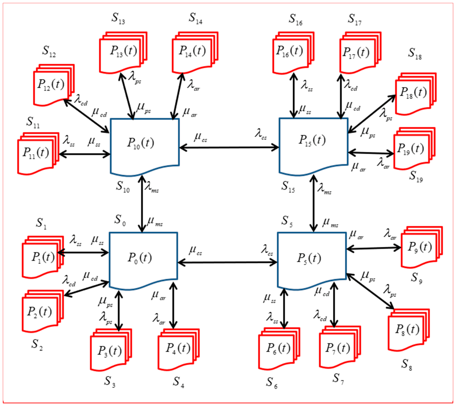
The following Figure 4 presents the state transition diagram of the Smart Residential Plant Bed Protection System (SRPBPS). This system consists of six subsystems, namely the sensing subsystem, monitoring and surveillance subsystem, control and decision subsystem, communication subsystem, alert and response subsystem, and power supply subsystem. Due to the failure of each subsystem, the system makes the transition from one state to another state. On the failure of the subsystem the repair team starts the repair of the failed subsystem. After the repair or replacement of the subsystem the system comes back in its working condition. Initially, the system is in the perfect working state $S_0$ and all the subsystems are working in perfect working condition. On the failure of the communication subsystem, or monitoring and surveillance subsystem, or both subsystems, the system operates in degraded states, which are presented by the states $\left(S_5,S_{10},S_{15}\right)$. All remaining states of the system are the failed states.

5. Origination of the Kolmogorov–Chapman Differential Equations of the Proposed System

In this section, the authors introduce the Kolmogorov–Chapman differential equations for the proposed system. Let the system make the transition from one state to another state in the time interval $\left(t,t+\Delta t\right)$ and now letting $\Delta t\to 0$, the following set of differential equations can be generated.

$$\begin{array}{l}\left[{\displaystyle \frac{d}{dt}}+{\lambda }_{ss}+{\lambda }_{cd}+{\lambda }_{ps}+{\lambda }_{ar}+{\lambda }_{cs}+{\lambda }_{ms}\right]P_0(t)={\mu }_{ss} P_1(t)+{\mu }_{cd} P_2(t)+{\mu }_{ps} P_3(t)+{\mu }_{ar} P_4(t)\\ +{\mu }_{cs} P_5(t)+{\mu }_{ms} P_{10}(t)\end{array}$$

(1)

$$\left[{\displaystyle \frac{d}{dt}}+{\mu }_{ss}\right]P_1(t)={\lambda }_{ss} P_0(t)$$

(2)

$$\left[{\displaystyle \frac{d}{dt}}+{\mu }_{cd}\right]P_2(t)={\lambda }_{cd} P_0(t)$$

(3)

$$\left[{\displaystyle \frac{d}{dt}}+{\mu }_{ps}\right]P_3(t)={\lambda }_{ps} P_0(t)$$

(4)

$$\left[{\displaystyle \frac{d}{dt}}+{\mu }_{ar}\right]P_4(t)={\lambda }_{ar} P_0(t)$$

(5)

$$\begin{array}{l}\left[{\displaystyle \frac{d}{dt}}+{\mu }_{cs}+{\lambda }_{ss}+{\lambda }_{cd}+{\lambda }_{ps}+{\lambda }_{ar}+{\lambda }_{ms}\right] P_5(t) ={\lambda }_{cs} P_0(t)+ {\mu }_{ss }{P}_6(t)+{\mu }_{cd} P_7(t)+{\mu }_{ps} P_8(t)\\ +{\mu }_{ar} P_9(t) +{\mu }_{ms} P_{15}(t)\end{array}$$

(6)

$$\left[{\displaystyle \frac{d}{dt}}+{\mu }_{ss}\right]P_6(t)={\lambda }_{ss} P_5(t)$$

(7)

$$\left[{\displaystyle \frac{d}{dt}}+{\mu }_{cd}\right]P_7(t)={\lambda }_{cd} P_5(t)$$

(8)

$$\left[{\displaystyle \frac{d}{dt}}+{\mu }_{ps}\right]P_8(t)={\lambda }_{ps} P_5(t)$$

(9)

$$\left[{\displaystyle \frac{d}{dt}}+{\mu }_{ar}\right]P_9(t)={\lambda }_{ar} P_5(t)$$

(10)

$$\begin{array}{l}\left[{\displaystyle \frac{d}{dt}}+{\mu }_{ms}+{\lambda }_{ss}+{\lambda }_{cd}+{\lambda }_{ps}+{\lambda }_{ar}+{\lambda }_{cs}\right] P_{10}(t)={\lambda }_{ms} P_0(t)+{\mu }_{ss} P_{11}(t)+{\mu }_{cd} P_{12}(t)+{\mu }_{ps} P_{13}(t)\\ +{\mu }_{ar} P_{14}(t)+{\mu }_{cs} P_{15}(t)\end{array}$$

(11)

$$\left[{\displaystyle \frac{d}{dt}}+{\mu }_{ss}\right]P_{11}(t)={\lambda }_{ss} P_{10}(t)$$

(12)

$$\left[{\displaystyle \frac{d}{dt}}+{\mu }_{cd}\right]P_{12}(t)={\lambda }_{cd} P_{10}(t)$$

(13)

$$\left[{\displaystyle \frac{d}{dt}}+{\mu }_{ps}\right]P_{13}(t)={\lambda }_{ps} P_{10}(t)$$

(14)

$$\left[{\displaystyle \frac{d}{dt}}+{\mu }_{ar}\right]P_{14}(t)={\lambda }_{ar} P_{10}(t)$$

(15)

$$\begin{array}{l}\left[{\displaystyle \frac{d}{dt}}+{\mu }_{cs}+{\lambda }_{ss}+{\lambda }_{cd}+{\lambda }_{ps}+{\lambda }_{ar}+{\mu }_{ms}\right] P_{15}(t)= {\lambda }_{cs} P_{10}(t)+{\mu }_{ss} P_{16}(t)+{\mu }_{cd} P_{17}(t)+{\mu }_{ps}{P}_{18}(t)\\ +{\mu }_{ar} P_{19}(t)+ {\lambda }_{ms} P_5(t)\end{array}$$

(16)

$$\left[{\displaystyle \frac{d}{dt}}+{\mu }_{ss}\right]P_{16}(t)={\lambda }_{ss} P_{15}(t)$$

(17)

$$\left[{\displaystyle \frac{d}{dt}}+{\mu }_{cd}\right]P_{17}(t)={\lambda }_{cd} P_{15}(t)$$

(18)

$$\left[{\displaystyle \frac{d}{dt}}+{\mu }_{ps}\right]P_{18}(t)={\lambda }_{ps} P_{15}(t)$$

(19)

$$\left[{\displaystyle \frac{d}{dt}}+{\mu }_{ar}\right]P_{19}(t)={\lambda }_{ar} P_{15}(t)$$

(20)

The initial condition is

$$P_i(0)=\left\{\begin{array}{cc}0& i\ne 0\\ 1& i=0\end{array}\right.$$

(21)

Taking the Inverse Laplace transformation of Equations (1) and (2), the following equations can be obtained.

$$\begin{array}{l}\left[s+{\lambda }_{ss}+{\lambda }_{cd}+{\lambda }_{ps}+{\lambda }_{ar}+{\lambda }_{cs}+{\lambda }_{ms}\right] {\overline{P}}_0(s)=1+{\mu }_{ss} {\overline{P}}_1(s)+{\mu }_{cd} {\overline{P}}_2(s)+{\mu }_{ps} {\overline{P}}_3(s)+{\mu }_{ar} {\overline{P}}_4(s)\\ +{\mu }_{cs} {\overline{P}}_5(s)+{\mu }_{ms} {\overline{P}}_{10}(s)\end{array}$$

(22)

$$\left[s+{\mu }_{ss}\right]{\overline{P}}_1(s)={\lambda }_{ss} {\overline{P}}_0(s)$$

(23)

$$\left[s+{\mu }_{cd}\right]{\overline{P}}_2(s)={\lambda }_{cd} {\overline{P}}_0(s)$$

(24)

$$\left[s+{\mu }_{ps}\right]{\overline{P}}_3(s)={\lambda }_{ps} {\overline{P}}_0(s)$$

(25)

$$\left[s+{\mu }_{ar}\right]{\overline{P}}_4(s)={\lambda }_{ar} {\overline{P}}_0(s)$$

(26)

$$\begin{array}{l}\left[s+{\mu }_{cs}+{\lambda }_{ss}+{\lambda }_{cd}+{\lambda }_{ps}+{\lambda }_{ar}+{\lambda }_{ms}\right] {\overline{P}}_5(s) ={\lambda }_{cs} {\overline{P}}_0(s)+ {\mu }_{ss }{\overline{P}}_6(s)+{\mu }_{cd} {\overline{P}}_7(s)+{\mu }_{ps} {\overline{P}}_8(s)\\ +{\mu }_{ar} {\overline{P}}_9(s) +{\mu }_{ms} {\overline{P}}_{15}(s)\end{array}$$

(27)

$$\left[s+{\mu }_{ss}\right]{\overline{ P}}_6(s)={\lambda }_{ss} {\overline{P}}_5(s)$$

(28)

$$\left[s+{\mu }_{cd}\right]{\overline{P}}_7(s)={\lambda }_{cd} {\overline{P}}_5(s)$$

(29)

$$\left[s+{\mu }_{ps}\right]{\overline{P}}_8(s)={\lambda }_{ps} {\overline{P}}_5(s)$$

(30)

$$\left[{\displaystyle \frac{d}{dt}}+{\mu }_{ar}\right]{\overline{P}}_9(s)={\lambda }_{ar} {\overline{P}}_5(s)$$

(31)

$$\begin{array}{l}\left[s+{\mu }_{ms}+{\lambda }_{ss}+{\lambda }_{cd}+{\lambda }_{ps}+{\lambda }_{ar}+{\lambda }_{cs}\right] {\overline{P}}_{10}(s)={\lambda }_{ms} {\overline{P}}_0(s)+{\mu }_{ss} {\overline{P}}_{11}(s)+{\mu }_{cd} {\overline{P}}_{12}(s)+{\mu }_{ps} {\overline{P}}_{13}(s)\\ +{\mu }_{ar} {\overline{P}}_{14}(s)+{\mu }_{cs} {\overline{P}}_{15}(s)\end{array}$$

(32)

$$\left[s+{\mu }_{ss}\right]{\overline{P}}_{11}(s)={\lambda }_{ss} {\overline{P}}_{10}(s)$$

(33)

$$\left[s+{\mu }_{cd}\right]{\overline{P}}_{12}(s)={\lambda }_{cd} {\overline{P}}_{10}(s)$$

(34)

$$\left[s+{\mu }_{ps}\right]{\overline{P}}_{13}(s)={\lambda }_{ps} {\overline{P}}_{10}(s)$$

(35)

$$\left[s+{\mu }_{ar}\right]{\overline{P}}_{14}(s)={\lambda }_{ar} {\overline{P}}_{10}(s)$$

(36)

$$\begin{array}{l}\left[s+{\mu }_{cs}+{\lambda }_{ss}+{\lambda }_{cd}+{\lambda }_{ps}+{\lambda }_{ar}+{\mu }_{ms}\right] {\overline{P}}_{15}(s)= {\lambda }_{cs} {\overline{P}}_{10}(s)+{\mu }_{ss} {\overline{P}}_{16}(s)+{\mu }_{cd} {\overline{P}}_{17}(s)+{\mu }_{ps}{\overline{P}}_{18}(s)\\ +{\mu }_{ar} {\overline{P}}_{19}(s)+ {\lambda }_{ms} {\overline{P}}_5(s)\end{array}$$

(37)

$$\left[s+{\mu }_{ss}\right]{\overline{P}}_{16}(s)={\lambda }_{ss} {\overline{P}}_{15}(s)$$

(38)

$$\left[s+{\mu }_{cd}\right]{\overline{P}}_{17}(s)={\lambda }_{cd} {\overline{P}}_{15}(s)$$

(39)

$$\left[s+{\mu }_{ps}\right]{\overline{P}}_{18}(s)={\lambda }_{ps} {\overline{P}}_{15}(s)$$

(40)

$$\left[s+{\mu }_{ar}\right]{\overline{P}}_{19}(s)={\lambda }_{ar} {\overline{P}}_{15}(s)$$

(41)

After solving these equations, the following state probabilities can be obtained.

$${\overline{P}}_0(s)={\displaystyle \frac{1}{Q_6}}$$

$${\overline{P}}_5(s)={\displaystyle \frac{{\mu }_{ms}{\lambda }_{ms}{\lambda }_{cs}}{Q_1{Q}_2{Q}_4}}{\overline{P}}_0(s)$$

$${\overline{P}}_{10}(s)={\displaystyle \frac{{\lambda }_{ms}}{Q_2}}{\overline{P}}_0(s)+{\displaystyle \frac{{\mu }_{cs}{\lambda }_{ms}}{Q_1{Q}_2}}{\overline{P}}_5(s)$$

$${\overline{P}}_{15}(s)={\displaystyle \frac{{\lambda }_{cs}}{Q_1}}{\overline{P}}_{10}(s)+{\displaystyle \frac{{\lambda }_{ms}}{Q_1}}{\overline{P}}_5(s)$$

where

$$Q_1=\left[s+{\mu }_{cs}+{\lambda }_{ss}+{\lambda }_{cd}+{\lambda }_{ps}+{\lambda }_{ar}+{\mu }_{ms}-{\displaystyle \frac{{\mu }_{ss}{\lambda }_{ss}}{s+{\mu }_{ss}}}-{\displaystyle \frac{{\mu }_{cd}{\lambda }_{cd}}{s+{\mu }_{cd}}}-{\displaystyle \frac{{\mu }_{ps}{\lambda }_{ps}}{s+{\mu }_{ps}}}-{\displaystyle \frac{{\mu }_{ar}{\lambda }_{ar}}{s+{\mu }_{ar}}}\right]$$

$$Q_2=\left[\begin{array}{l}s+{\mu }_{ms}+{\lambda }_{ss}+{\lambda }_{cd}+{\lambda }_{ps}+{\lambda }_{ar}+{\lambda }_{cs}-{\displaystyle \frac{{\mu }_{ss}{\lambda }_{ss}}{s+{\mu }_{ss}}}-{\displaystyle \frac{{\mu }_{cd}{\lambda }_{cd}}{s+{\mu }_{cd}}}-{\displaystyle \frac{{\mu }_{ps}{\lambda }_{ps}}{s+{\mu }_{ps}}}-{\displaystyle \frac{{\mu }_{ar}{\lambda }_{ar}}{s+{\mu }_{ar}}}\\ -{\displaystyle \frac{{\lambda }_{cs}{\mu }_{cs}}{Q_1}}\end{array}\right]$$

$$Q_3=\left[\begin{array}{l}s+{\mu }_{cs}+{\lambda }_{ss}+{\lambda }_{cd}+{\lambda }_{ps}+{\lambda }_{ar}+{\lambda }_{ms}-{\displaystyle \frac{{\mu }_{ss}{\lambda }_{ss}}{s+{\mu }_{ss}}}-{\displaystyle \frac{{\mu }_{cd}{\lambda }_{cd}}{s+{\mu }_{cd}}}-{\displaystyle \frac{{\mu }_{ps}{\lambda }_{ps}}{s+{\mu }_{ps}}}-{\displaystyle \frac{{\mu }_{ar}{\lambda }_{ar}}{s+{\mu }_{ar}}}\end{array}\right]$$

$$Q_4=\left[\begin{array}{l}{Q}_3-{\displaystyle \frac{{\mu }_{ms}{\lambda }_{cs}{\mu }_{cs}{\lambda }_{ms}}{Q_1^2{Q}_2}}-{\displaystyle \frac{{\mu }_{ms}{\lambda }_{ms}}{Q_1}}\end{array}\right]$$

$$Q_5=\left[\begin{array}{l}s+{\lambda }_{ss}+{\lambda }_{cd}+{\lambda }_{ps}+{\lambda }_{ar}+{\lambda }_{cs}+{\lambda }_{ms}-{\displaystyle \frac{{\mu }_{ss}{\lambda }_{ss}}{s+{\mu }_{ss}}}-{\displaystyle \frac{{\mu }_{cd}{\lambda }_{cd}}{s+{\mu }_{cd}}}-{\displaystyle \frac{{\mu }_{ps}{\lambda }_{ps}}{s+{\mu }_{ps}}}-{\displaystyle \frac{{\mu }_{ar}{\lambda }_{ar}}{s+{\mu }_{ar}}}\end{array}\right]$$

$$Q_6=\left[\begin{array}{l}{Q}_5-{\displaystyle \frac{{\mu }_{cs}{\mu }_{ms}{\lambda }_{ms}{\lambda }_{cs}}{Q_1{Q}_2{Q}_4}}-{\displaystyle \frac{{\mu }_{ms}{\lambda }_{ms}}{Q_2}}-{\displaystyle \frac{{\mu }_{ms}^2{\lambda }_{ms}^2{\mu }_{cs}{\lambda }_{cs}}{Q_1^2{Q}_2^2{Q}_4}}\end{array}\right]$$

The proposed system (SRPBPS) at any time ‘t’ can always be in either the working state or in the failed state. Hence, the probability of the system being in the working state is known as the probability of upstate and it is the sum total of all probabilities of the system in which system is working. The upstate probability of the system is given in Equation (42).

$${\overline{P}}_{up}\left(s\right)={\overline{P}}_0\left(s\right)+{\overline{P}}_5\left(s\right)+{\overline{P}}_{10}\left(s\right)+{\overline{P}}_{15}\left(s\right)$$

(42)

Similarly, the probability of the system being in the failed state is known as the probability of downstate, and it is the sum total of all probabilities in which the system is not working. The downstate probability of the system is given in Equation (43).

$${\overline{P}}_{downtime}(s)={\sum }_{i=1}^{i=4}{\overline{P}}_i(s)+{\sum }_{i=6}^{i=9}{\overline{P}}_i(s)+{\sum }_{i=11}^{i=14}{\overline{P}}_i(s)+{\sum }_{i=16}^{i=19}{\overline{P}}_i(s)$$

(43)

The failure and repair rates utilized in

Table 2. Failure and Repair rate data.

Subsystem	Failure Rate/hrs	Repair Rate/hrs
Sensing subsystem	${\lambda }_{ss}=0.0003$	${\mu }_{ss}=0.8$
Monitoring and surveillance subsystem	${\lambda }_{ms}=0.0002$	${\mu }_{ms}=0.7$
Control and decision subsystem	${\lambda }_{cd}=0.0008$	${\mu }_{cd}=0.6$
Communication subsystem	${\lambda }_{cs}=0.00015$	${\mu }_{cs}=1$
Alert and response subsystem	${\lambda }_{ar}=0.00012$	${\mu }_{ar}=1.2$
Power supply	${\lambda }_{ps}=0.0004$	${\mu }_{ps}=0.4$

were calculated using expert opinion and engineering judgement because there was no published reliability data or comparable model for the suggested IoT-based plant protection system in the literature. These values were chosen to illustrate the suggested model’s performance and applicability.

6. Performance Measurement of the Proposed Smart Residential Plant Bed Protection System

In this section, the authors have calculated the various reliability measures of the Smart Residential Plant Bed Protection System. The system reliability and MTTF have been calculated. Also, sensitivity analyses of the MTTF and reliability have been performed to determine the most critical components of the system. In the end, authors have calculated expected number of failures of the system for the total time duration of 5000 h.

6.1. Reliability of the Smart Residential Plant Bed Protection System

Reliability is defined as the probability that the system will perform its intended task for the prescribed period of time when operated under the specified condition. Let the random variable T be defined as the time to failure of the system. Mathematically, the reliability of the system is given by Equation (44), it describes that the system cannot fail before the time period ‘t’.

$$R(t)=P(T>t)$$

(44)

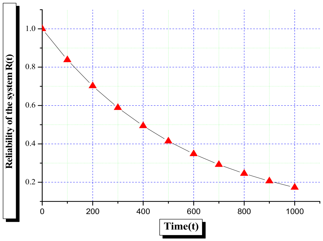
For calculating the reliability of the proposed system set all repair rates values zero in Equation (42), and also set failure rate values as ${\lambda }_{ss}=0.0003,$ ${\lambda }_{ms}=0.0002,$ ${\lambda }_{cd}=0.0008,$ ${\lambda }_{cs}=0.00015,$ ${\lambda }_{ar}=0.00012,$ ${\lambda }_{ps}=0.0004$. On taking the inverse Laplace transformation of the equation, the expression for the time dependent reliability can be obtained as given in Equation (45).

$$\begin{array}{l}R(t)= 1.428571429 e^{-0.00197 t}+2 e^{-0.00187 t} \sinh (0.0001 t)+0.5714285714 e^{-0.00162 t}\\ - e^{-0.00177 t}\end{array}$$

(45)

By varying the time unit ‘t’ from 0 to 1000 h,

Table 3. Time v/s reliability of the system.

Time $\mathit{t}$ (In Hours)	Reliability R(t)
0	1.0000
100	0.8379
200	0.7022
300	0.5888
400	0.4938
500	0.4142
600	0.3476
700	0.2918
800	0.2450
900	0.2057
1000	0.1728

and Figure 5 can be obtained.

6.2. Mean Time to First Failure (MTTF) of the Smart Residential Plant Bed Protection System

Another important measure of the system’s performance is the mean time to the first failure of the system. If the value of this measure is smaller, then the chances are high that this product will fail soon, and hence it is considered unreliable. On the contrary bigger value of this measure indicates that chances are very low that this product will fail soon. Now to compute the MTTF of the system, set all the failure rates equal to zero in Equation (42), and then taking the limit $s\to 0$, the expression for the system’s MTTF can be obtained as given below in Equation (46).

$$MTTF= \left[\begin{array}{l}{\displaystyle \frac{1}{{\lambda }_{ss}+{\lambda }_{cd}+{\lambda }_{ps}+{\lambda }_{ar}+{\lambda }_{cs}+{\lambda }_{ms}}}\\ +{\displaystyle \frac{{\lambda }_{ms}}{\left({\lambda }_{ss}+{\lambda }_{cd}+{\lambda }_{ps}+{\lambda }_{ar}+{\lambda }_{cs}\right)\left({\lambda }_{ss}+{\lambda }_{cd}+{\lambda }_{ps}+{\lambda }_{ar}+{\lambda }_{cs}+{\lambda }_{ms}\right)}}\\ +{\displaystyle \frac{{\lambda }_{cs}{\lambda }_{ms}}{\left({\lambda }_{ss}+{\lambda }_{cd}+{\lambda }_{ps}+{\lambda }_{ar}\right)\left({\lambda }_{ss}+{\lambda }_{cd}+{\lambda }_{ps}+{\lambda }_{ar}+{\lambda }_{cs}\right)\left({\lambda }_{ss}+{\lambda }_{cd}+{\lambda }_{ps}+{\lambda }_{ar}+{\lambda }_{cs}+{\lambda }_{ms}\right)}}\end{array}\right]$$

(46)

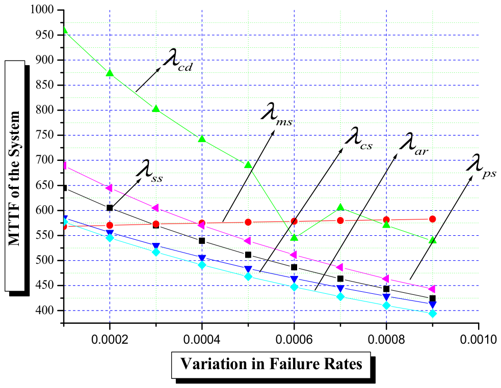
Now set the failure rate values as ${\lambda }_{ss}=0.0003,$ ${\lambda }_{ms}=0.0002,$ ${\lambda }_{cd}=0.0008,$ ${\lambda }_{cs}=0.00015,$ ${\lambda }_{ar}=0.00012,$ ${\lambda }_{ps}=0.0004$. By varying each failure rate from 0.0001 to 0.0009 by keeping the other failure rates fixed,

Table 4. Variation in failure rates vs. MTTF.

Variation in the Failure Rates	${\mathit{\lambda }}_{\mathit{s}\mathit{s}}$	${\mathit{\lambda }}_{\mathit{m}\mathit{s}}$	${\mathit{\lambda }}_{\mathit{c}\mathit{d}}$	${\mathit{\lambda }}_{\mathit{c}\mathit{s}}$	${\mathit{\lambda }}_{\mathit{a}\mathit{r}}$	${\mathit{\lambda }}_{\mathit{p}\mathit{s}}$
0.0001	644.54	567.76	958.57	585.13	576.92	689.53
0.0002	605.12	570.28	873.04	556.16	545.19	644.54
0.0003	570.28	572.55	801.74	529.93	516.79	605.12
0.0004	539.26	574.61	741.35	506.06	491.22	570.28
0.0005	511.47	576.49	689.53	484.24	468.08	539.26
0.0006	486.41	578.21	544.54	464.23	447.03	511.47
0.0007	463.71	579.79	605.12	445.81	427.80	486.41
0.0008	443.05	581.25	570.28	428.80	410.17	463.71
0.0009	424.15	582.60	539.26	413.03	393.93	443.05

and Figure 6 of MTTF of the system can be obtained.

6.3. Sensitivity Analysis of Mean Time to First Failure (MTTF) of the Smart Residential Plant Bed Protection System

Sensitivity analysis of the MTTF is performed to determine which component’s failure rate, when increased, affects the system’s MTTF the most. For performing the sensitivity analysis of the MTTF of the system, differentiate Equation (46) w.r.t the failure rates one by one and then set all failure rates value as:

$$\begin{gathered} {\lambda }_{ss}=0.0003, {\lambda }_{ms}=0.0002, {\lambda }_{cd}=0.0008, {\lambda }_{cs}=0.00015, {\lambda }_{ar}=0.00012, \\ {\lambda }_{ps}=0.0004 \end{gathered}$$

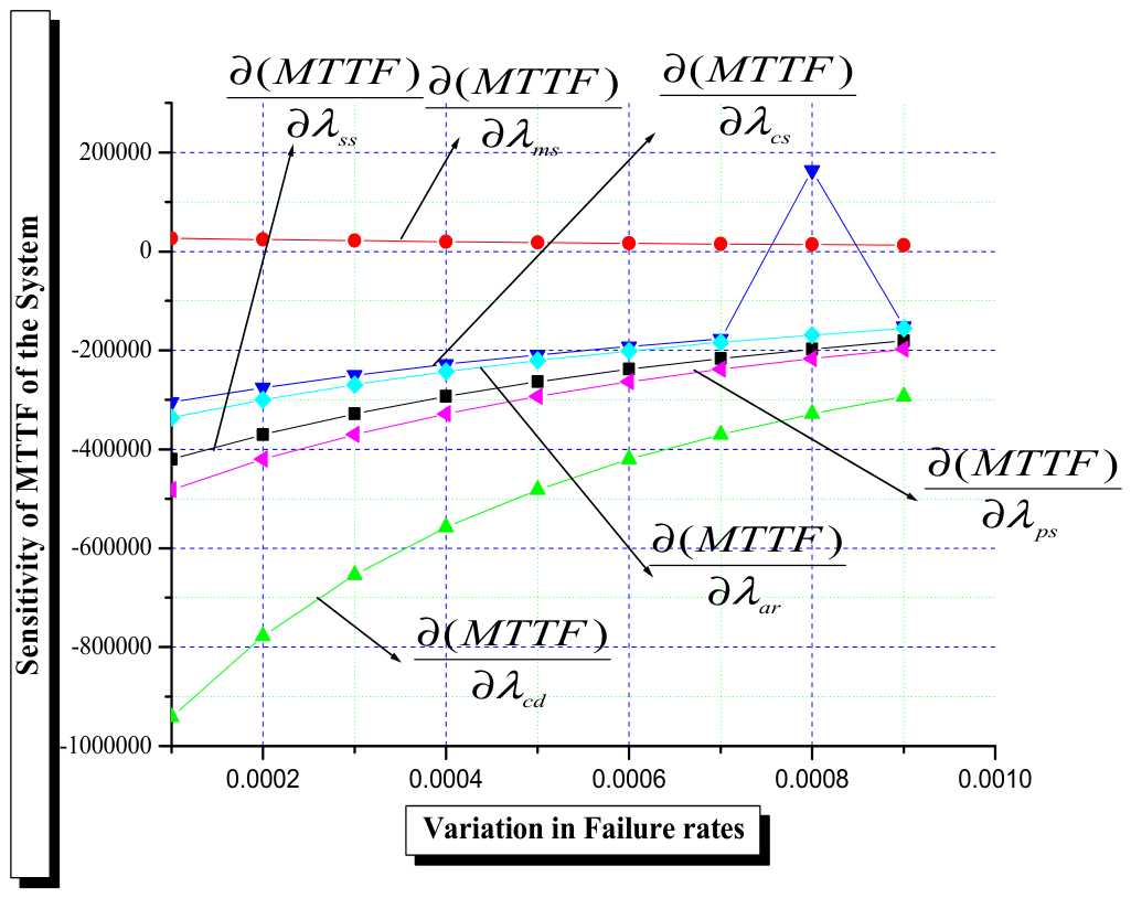
By varying each failure rate value from 0.0001 to 0.0009, by keeping the other failure rate values fixed,

Table 5. Variation in failure rates vs. sensitivity of MTTF of the system.

Variation in the Failure Rates	$\frac{\partial \left(\mathit{M}\mathit{T}\mathit{T}\mathit{F}\right)}{\partial {\mathit{\lambda }}_{\mathit{s}\mathit{s}}}$	$\frac{\partial \left(\mathit{M}\mathit{T}\mathit{T}\mathit{F}\right)}{\partial {\mathit{\lambda }}_{\mathit{m}\mathit{s}}}$	$\frac{\partial \left(\mathit{M}\mathit{T}\mathit{T}\mathit{F}\right)}{\partial {\mathit{\lambda }}_{\mathit{c}\mathit{d}}}$	$\frac{\partial \left(\mathit{M}\mathit{T}\mathit{T}\mathit{F}\right)}{\partial {\mathit{\lambda }}_{\mathit{c}\mathit{s}}}$	$\frac{\partial \left(\mathit{M}\mathit{T}\mathit{T}\mathit{F}\right)}{\partial {\mathit{\lambda }}_{\mathit{a}\mathit{r}}}$	$\frac{\partial \left(\mathit{M}\mathit{T}\mathit{T}\mathit{F}\right)}{\partial {\mathit{\lambda }}_{\mathit{p}\mathit{s}}}$
0.0001	−420,187.51	26,478.47	−940,843.09	−304,757.15	−335,922.09	−481,625.29
0.0002	−369,886.37	23,858.53	−777,579.34	−275,330.06	−299,706.26	−420,187.51
0.0003	−328,167.78	21,609.04	−653,869.42	−249,968.13	−269,081.05	−369,886.37
0.0004	−293,173.60	19,663.31	−557,791.07	−227,955.68	−242,946.54	−328,167.78
0.0005	−263,525.01	17,969.02	−481,625.29	−208,727.85	−220,461.74	−293,173.60
0.0006	−238,180.83	16,484.64	−420,187.52	−191,834.02	−200,974.46	−263,525.01
0.0007	−216,342.64	15,176.87	−369,886.37	−176,911.18	−183,972.47	−238,180.83
0.0008	−197,389.59	14,018.77	−328,167.78	163,664.23	−169,048.85	−216,342.64
0.0009	−180,832.95	12,988.34	−293,173.60	−151,851.31	−155,876.95	−197,389.59

and Figure 7 are obtained.

6.4. Sensitivity Analysis of Reliability of the Smart Residential Plant Bed Protection System

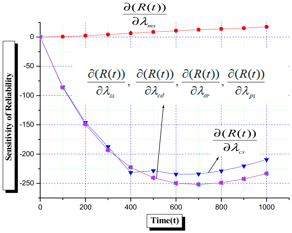
Sensitivity analysis of the reliability is performed to determine which component’s failure rate when increased affects the system’s reliability the most when time t increases. For performing the sensitivity analysis of the reliability of the system, set all repair rates equal to zero in Equation (42) and then take Inverse Laplace transformation of this equation. For this obtained equation differentiate it w.r.t each failure rate and set the failure rate values as ${\lambda }_{ss}=0.0003,$ ${\lambda }_{ms}=0.0002,$ ${\lambda }_{cd}=0.0008,$ ${\lambda }_{cs}=0.00015,$ ${\lambda }_{ar}=0.00012$ ${\lambda }_{ps}=0.0004$ then varying the time unit t from 0 to 1000, the following

Table 6. Time vs. Sensitivity of reliability.

Time t In hours.	$\frac{\partial \left(\mathit{R}\right(\mathit{t}\left)\right)}{\partial {\mathit{\lambda }}_{\mathit{s}\mathit{s}}}$	$\frac{\partial \left(\mathit{R}\right(\mathit{t}\left)\right)}{\partial {\mathit{\lambda }}_{\mathit{m}\mathit{s}}}$	$\frac{\partial \left(\mathit{R}\right(\mathit{t}\left)\right)}{\partial {\mathit{\lambda }}_{\mathit{c}\mathit{d}}}$	$\frac{\partial \left(\mathit{R}\right(\mathit{t}\left)\right)}{\partial {\mathit{\lambda }}_{\mathit{c}\mathit{s}}}$	$\frac{\partial \left(\mathit{R}\right(\mathit{t}\left)\right)}{\partial {\mathit{\lambda }}_{\mathit{a}\mathit{r}}}$	$\frac{\partial \left(\mathit{R}\right(\mathit{t}\left)\right)}{\partial {\mathit{\lambda }}_{\mathit{p}\mathit{s}}}$
0	0	0	0	0	0	0
100	−86.34	0.64	−86.34	−85.47	−86.34	−86.34
200	−149.14	2.18	−149.14	−146.14	−149.14	−149.14
300	−193.27	4.24	−193.27	−187.42	−193.27	−193.27
400	−222.70	6.45	−222.70	−231.69	−222.70	−222.70
500	−240.64	8.63	−240.64	−228.44	−240.64	−240.64
600	−249.70	10.64	−249.70	−234.47	−249.70	−249.70
700	−251.97	12.40	−251.97	−234.02	−251.97	−251.97
800	−249.15	13.88	−249.15	−228.82	−249.15	−249.15
900	−242.57	15.05	−242.57	−220.28	−242.57	−242.57
1000	−233.32	17.38	−233.32	−209.47	−233.32	−233.32

and Figure 8 can be obtained.

6.5. Expected Number of Failures of the Smart Residential Plant Bed Protection System

The expected number of system failures $E\left[N\right(t\left)\right]$ represents the average number of times a system fails during a specified time interval $\left[0,t\right]$. It is widely used for repairable systems, where failures can occur multiple times and the system is restored after each failure. This helps in evaluating system performance, planning maintenance schedules, and estimating operational costs. It depends on the failure intensity function $\lambda \left(t\right)$ which describes how frequently failures occur over time. A higher expected number indicates lower reliability and poorer system performance. To calculate the Expected number of system’s failure set the failure rate values as ${\lambda }_{ss}=0.0003,$ ${\lambda }_{ms}=0.0002,$ ${\lambda }_{cd}=0.0008,$ ${\lambda }_{cs}=0.00015,$ ${\lambda }_{ar}=0.00012,$ ${\lambda }_{ps}=0.0004$ in Equation (46).

After that multiply the obtained MTTF by the time unit $t$, as shown in Equation (47).

$$EN\left[t\right]=t.MTTF$$

(47)

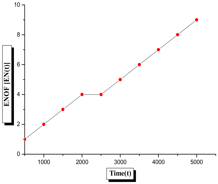
This gives the expected number of failures which can occur in the time interval $\left[0,t\right]$. The associated results are shown in the following

Table 7. Time vs. Expected Number of system Failures.

Time t (In Hours)	$\mathit{E}\left[\mathit{N}\right(\mathit{t}\left)\right]$
500	1
1000	2
1500	3
2000	4
2500	4
3000	5
3500	6
4000	7
4500	8
5000	9

and Figure 9.

7. Results and Discussion

In this section, the authors present the results obtained in the above Section 6. The authors calculated the various reliability measures of the Smart Residential Plant Bed Protection System (SRPBPS). To monitor plant beds and warn the homeowner when suspicious activity takes place, the system incorporates motion sensors, plant disturbance sensors, a video module, a microcontroller unit, a communication module, and an alarm mechanism. For the proper functioning of this system, it is mandatory that all the components of the system work properly. The following results have been obtained from the above section.

Table 3 and Figure 5 show that the system reliability decreases steadily with time, from 1.0000 initially to 0.1728 after 1000 h. The maximum decline occurs within the first 100 h (16.2% reduction). Reliability drops below 50% between 400 and 500 h and falls under 0.35 after 600 h. The smooth decline indicates a stable and predictable aging behaviour of the system.

Table 4 and Figure 6 present the variation in MTTF with increasing failure rates. The MTTF of most subsystems decreases monotonically as the failure rate rises from 0.0001 to 0.0009. The alert and response subsystem consistently exhibits the lowest MTTF, followed by the communication subsystem, indicating high vulnerability to failures. In contrast, the monitoring and surveillance subsystem shows the lowest MTTF only at the minimum failure rate and then improves gradually, while the control and decision subsystem exhibits non-monotonic behaviour. These findings identify the alert and response subsystem and communication subsystem as the most failure-prone components.

Table 5 and Figure 7 illustrate the sensitivity of MTTF with respect to subsystem failure rates. The control and decision subsystem is the most sensitive component, showing the highest impact on MTTF across all variations. The power supply and sensing subsystems also significantly influence system performance. Conversely, the monitoring and surveillance subsystem has the least sensitivity, indicating minimal effect on overall MTTF.

Table 6 and Figure 8 show the sensitivity of system reliability with respect to time variation. The sensing, control and decision, alert and response, and power supply subsystems exhibit the highest and nearly identical sensitivity magnitudes, making them equally critical to system reliability. The communication subsystem also has a strong influence, whereas the monitoring and surveillance subsystem demonstrates the lowest sensitivity and comparatively smaller impact on reliability

Table 7 and Figure 9 show that the expected number of system failures increases nearly linearly with time, from 1 at 500 h to 9 at 5000 h, indicating an approximately constant failure rate. A short plateau between 2000 and 2500 h suggests a temporary improvement in reliability. After 2500 h, failures increase steadily again, reflecting gradual system degradation and supporting a non-homogeneous Poisson failure process.

8. Conclusions

The proposed Smart Residential Plant Bed Protection System (SRPBPS) offer a structured, reliability-driven solution to prevent unauthorized plucking from household plant beds. The Markov-based reliability analysis reveals that the system’s reliability decays steadily over time, reaching 50% between 400 and 500 h, with a predictable ageing pattern that facilitates maintenance scheduling. The mean time to first failure (MTTF) and sensitivity analyses consistently identify the alert and response subsystem and control and decision subsystem as the most failure-sensitive components, exhibiting the lowest MTTF under increasing failure rates. Moreover, the control and decision subsystem, sensing subsystem, alert and response subsystem and power supply subsystem show the high sensitivity in reliability, making them equally critical to overall system performance. In contrast, the monitoring and surveillance subsystem has the least influence on system reliability. The expected number of system failures increases nearly linearly but shows a temporary plateau (2000–2500 h), indicating intermittent periods of improved reliability. Control and Decision, as well as the Alert and Response Subsystem are the most critical elements of the SRPBPS and should receive the highest priority for redundancy, fault tolerance, and maintenance. The dependability, availability, and operational lifetime of the system will be greatly increased by improving these components as well as the sensing, communication, and power supply subsystems. The proposed framework not only advances smart gardening security but also provides a replicable methodology for reliability assessment of similar IoT-based residential protection system.

9. Future Scopes

• Develop a centralized dashboard with push notifications to provide homeowners with live system health and failure predictions, enabling quicker manual intervention before component breakdowns.
• Integrate solar or vibration energy harvesting with battery backup into the critical power and communication subsystems, ensuring continuous operation during grid outages or lowpower conditions.
• Future work will focus on developing and testing a real prototype of the SRPBPS to validate the analytical results using performance metrics such as detection accuracy, false alarm rate, response time, and energy consumption. Redundancy, maintenance plans, and comparisons with other reliability assessment methods are additional ways to expand the model.

References

1. Dhillon, B.S. Engineering Maintenance: A Modern Approach; CRC Press: Boca Raton, FL, USA, 2002. [Google Scholar]
2. Ebeling, C.E. An Introduction to Reliability and Maintainability Engineering; Waveland Press: Long Grove, IL, USA, 2019. [Google Scholar]
3. Srinath, L.S. Reliability Engineering; Affiliated East-West Press: New Delhi, Delhi, 1991; pp. 1641–1654. [Google Scholar]
4. van der Ree, R. Barbed wire fencing as a hazard for wildlife. Victorian Nat. 1999, 116, 210–217. [Google Scholar]
5. Burudi, J.W.; Tormáné Kovács, E.; Katona, K. Wildlife fences to mitigate human–wildlife conflicts in Africa: A literature analysis. Diversity 2025, 17, 87. [Google Scholar] [CrossRef]
6. Campbell, D.L.; Lea, J.M.; Keshavarzi, H.; Lee, C. Virtual fencing is comparable to electric tape fencing for cattle behavior and welfare. Front. Vet. Sci. 2019, 6, 445. [Google Scholar] [CrossRef] [PubMed]
7. Savović, S.; Savović, M.; Deng, X. Stochastic modeling of mode coupling and steady-state performance in multimode plastic optical fibers for telecom applications. Telecom 2026, 7, 62. [Google Scholar] [CrossRef]
8. Su, C.; Chen, W. Design of Remote Real-Time Monitoring and Control Management System for Smart Home Equipment Based on Wireless Multihop Sensor Network. J. Sens. 2022, 2022, 6228440. [Google Scholar] [CrossRef]
9. May, Z.B. Real-time alert system for home surveillance. In Proceedings of the 2012 IEEE International Conference on Control System, Computing and Engineering, Penang, Malaysia, 23–25 November 2012; IEEE: Piscataway, NJ, USA, 2012; pp. 501–505. [Google Scholar]
10. Keat, L.H.; Wen, C.C. Smart indoor home surveillance monitoring system using Raspberry Pi. JOIV Int. J. Inform. Vis. 2018, 2, 299–308. [Google Scholar]
11. Dey, S.; Kundu, T.; Mukherjee, S.; Sarkar, M. Web based real-time home automation and security system. Int. J. Electr. Electron. Eng. Telecommun. 2015, 4, 1–8. [Google Scholar]
12. Haxhismajli, B.; Marinova, G.; Hajrizi, E.; Qehaja, B. Unsupervised deep learning-based network traffic anomaly detection for DDoS mitigation in smart microgrid communication infrastructure. Telecom 2026, 7, 58. [Google Scholar] [CrossRef]
13. Ram, M. On system reliability approaches: A brief survey. Int. J. Syst. Assur. Eng. Manag. 2013, 4, 101–117. [Google Scholar] [CrossRef]
14. Maihulla, A.S.; Yusuf, İ.; Koo, M.B.C. Reliability and availability analyses of an industrial system with two subsystems arranged in series-parallel. Sigma J. Eng. Nat. Sci. 2024, 42, 1500–1510. [Google Scholar] [CrossRef]
15. Musa, M.A.; Yusuf, I.; Liman, M.; Rumu, Y.S. A performance measure of centrifugal water pumping system’s reliability, availability, maintainability and dependability. Int. J. Process Manag. Benchmarking 2025, 19, 320–349. [Google Scholar] [CrossRef]
16. Kumar, P.; Kumar, A.; Chhetri, G. Reliability Centered Modeling of an Automated Waste Sorting Robotic Arm System. Int. J. Math. Eng. Manag. Sci. 2024, 9, 1210–1225. [Google Scholar] [CrossRef]
17. Kumar, P.; Kumar, A.; Sharma, S. Understanding Reliability indices of a Seabin for Automated Water Cleaning through Markov State based Modelling. J. Reliab. Stat. Stud. 2025, 18, 243–270. [Google Scholar] [CrossRef]
18. Kishor, A.; Yadav, S.P.; Kumar, S. A multi-objective genetic algorithm for reliability optimization problem. Int. J. Perform. Eng. 2009, 5, 227. [Google Scholar]
19. Sharma, S.; Kumar, V. Reliability estimation in a two-unit hot standby system under classical and Bayesian inferential framework. Proc. Inst. Mech. Eng. Part O J. Risk Reliab. 2026, 240, 105–120. [Google Scholar] [CrossRef]
20. Liu, J.; Li, Y.; Ma, X.; Wang, L.; Li, J. Fault tree analysis using Bayesian optimization: A reliable and effective fault diagnosis approaches. J. Fail. Anal. Prev. 2021, 21, 619–630. [Google Scholar] [CrossRef]
Figure 1. Urban Gardening Cycle.
Telecom 07 00076 g001
Figure 2. Perfect working state, degraded state, and failed state of the system.
Telecom 07 00076 g002
Figure 3. Plant Protection System architecture.
Telecom 07 00076 g003
Figure 4. State transition diagram of the Smart Residential Plant Bed Protection System (SRPBPS).
Telecom 07 00076 g004
Figure 5. Time vs. reliability of the system.
Telecom 07 00076 g005
Figure 6. Variation in failure rates vs. MTTF.
Telecom 07 00076 g006
Figure 7. Variation in failure rates vs. sensitivity of MTTF of the system.
Telecom 07 00076 g007
Figure 8. Time vs. Sensitivity of reliability.
Telecom 07 00076 g008
Figure 9. Time vs. expected number of system failures.
Telecom 07 00076 g009