Article

MAOA: A Swift and Effective Optimization Algorithm for Linear Antenna Array Design

1
Department of Electrical and Electronics Engineering, University of Petroleum and Energy Studies, Dehradun 248007, Uttarakhand, India
2
Department of ECE, Birla Institute of Applied Sciences, Bhimtal 263136, Uttarakhand, India
3
Paras Antidrone Technologies Private Limited, Navi Mumbai 400706, Maharashtra, India
4
Department of Computer Science and Engineering, Graphic Era Deemed to Be University, Dehradun 248002, Uttarakhand, India
5
Faculty of Engineering, Technology and Built Environment, UCSI University, Kuala Lumpur 56000, Malaysia
*
Authors to whom correspondence should be addressed.
Telecom 2025, 6(2), 34; https://doi.org/10.3390/telecom6020034
Submission received: 1 April 2025 / Revised: 16 May 2025 / Accepted: 20 May 2025 / Published: 23 May 2025

Abstract

:
This paper presents the modified arithmetic optimization algorithm (MAOA), a swift and effective optimization algorithm specifically designed for electromagnetic applications. Its primary advantage is its ability to avoid local minima by striking a balance between global exploration and local exploitation searches. This equilibrium is maintained through three key improvements: an enhanced initialization process, a distinctive guidance mechanism for steering searches, and an additional learning phase to refine newly found solutions. This process innovation significantly boosts MAOA’s performance in addressing both constrained and unconstrained optimization challenges. In this study, MAOA is applied to optimize the spacing and current amplitude of linear antenna array (LAA) elements, with the goal of minimizing peak side lobe level (PSLL), close-in side lobe level (CSLL), and overall side lobe level (SLL), both with and without constraints on first null beamwidth (FNBW), as well as null positioning with SLL minimization. Ten designs, comprising 10 and 20 antenna elements of LAA and one 14-element circular antenna array (CAA), showcase MAOA’s proficiency in antenna array pattern synthesis. Optimizing element positions results in a PSLL of −21.28 dB, a CSLL of −34.50 dB, and a null depth of −89.00 dB, while optimizing current amplitude achieves a PSLL of −24.32 dB, a CSLL of −29.73 dB, and a null depth of −77.60 dB across various antenna designs. Simulation results reveal that MAOA significantly surpasses traditional uniform linear arrays (ULA) and established optimization techniques. Its superiority is further confirmed through a Wilcoxon rank-sum and Friedman test.

1. Introduction

The rapid evolution in the field of communication technology significantly affects the routine behavior of humans in society. The widespread adoption of mobile communication is profoundly shaping modern lifestyles [
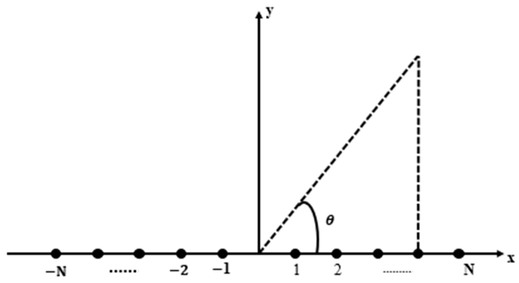
1]. In this dynamic environment, the importance of efficient antenna systems cannot be overstated, but their design and synthesis remain a complex and challenging task. One of the most sought-after and adopted layouts for this purpose is the linear antenna array (LAA); in its configuration, the number of antenna elements is placed in a linear fashion [2]. Estimating the parameters of these antenna arrays for obtaining the desired radiation performance is called pattern synthesis. Mostly, the system is required to maintain a low SLL to overcome the interference effect that occurs with adjacent systems working within the same frequency range. A narrow first null beamwidth (FNBW) is also desired in the antenna array system, so that it shows a high level of directivity during its operation [3]. Satisfying both the conditions of low SLL and narrow beamwidth simultaneously is very tedious work, because both aspects are dependent on each other. Improving one aspect may degrade the performance of the other [4]. In many situations, the beamwidth and the system gain are compromised to reduce the SLL [5]. The other requirement from the antenna array is that it should place the deeper nulls in the intended direction, so that the interfering sources are avoided, but a large electromagnetic population hinders these placements to a greater extent [6]. So, the major aspects which are required in an antenna array are that it must have a low side lobe level with constant FNBW and that the nulls are oriented toward the directions from where the interference is coming from. The parameters that affect the radiation performance of an antenna array are the shape of the array, interelement spacing of the elements, current amplitude, and its phase [7]. In an LAA, SLL minimization and placement of nulls in the desired direction are obtained by using two methods [8]. The first is by optimizing the interelement spacing considering uniform current excitation; the second is by fixing the spacing constant and optimizing the amplitude of the excitation current [9].
The optimization strategies are broadly classified into deterministic and stochastic techniques. The deterministic approach requires a good initial guess for its implementation, and its computational time is too high when handling complex optimization problems. Also, this type of approach is highly sensitive and prone to being confined in the local minima [10]. However, stochastic approaches, which include metaheuristic algorithms, are mostly applied to handle complex optimization scenarios. Many developed metaheuristic approaches are influenced by natural phenomena and swarm intelligence [11]. These approaches are well suited for performing pattern synthesis in an antenna array [12]. Some of the evolutionary optimization algorithms applied to handle the electromagnetic problems of an antenna array are as follows: atom search [13,14], BAT algorithm [15,16], bacterial foraging [17], CAT swarm [2,18,19], dragonfly algorithm (DA) [20], flower pollination [21], grey wolf optimization (GWO) [11,12,22], moth flame optimization (MFO) [23], particle swarm optimization (PSO) [4,24], social group optimization algorithm [25], Taguchi [8,26], biogeography based optimization (BBO) [27], ant lion optimization (ALO) [28], spider monkey optimization [29], and many more. These smart algorithms are also helpful in optimizing the parameters of other kinds of antenna array configurations, such as concentric [30], conformal [31], and circular [32] antenna arrays. Moreover, in [33], the author explored swarm intelligence algorithms to improve the performance of multiple-input and multiple-output (MIMO) antennas [34,35].
The arithmetic optimization algorithm (AOA) is a recently proposed metaheuristic algorithm by Abualigah et al. in 2021 [34]. The search mechanisms of AOA are influenced by the diverse distributive characteristics of four fundamental arithmetic functions known as division, multiplication, addition, and subtraction. These arithmetic operators are employed in AOA along with its unique mechanisms to balance exploration and exploitation in searching for new solutions within the solution space. Specifically, the division and multiplication operators promote exploration, enabling the population to navigate broader regions of the search space and identify more promising solutions. In contrast, the addition and subtraction operators facilitate exploitation, refining already discovered promising solution areas. Since its inception, AOA has gained recognition as a popular metaheuristic algorithm for solving a variety of real-world optimization problems [35,36,37,38,39]. However, like other metaheuristic algorithms, AOA also suffers from some inherent shortcomings. The first shortcoming is the questionable quality of the initial population proposed by the stochastic-based conventional initialization techniques. The second limitation involves the over-reliance on the current best solution to direct the search procedure for all population members of AOA when using the four arithmetic operators. Additionally, the lack of a sophisticated learning phase within the AOA framework may limit its ability to prevent solutions from getting stuck in local optima. These shortcomings can impact the resilience of AOA, leading to early convergence, particularly when addressing complex optimization issues with challenging fitness landscapes, and resulting in suboptimal outcomes.
In this paper, an MAOA is proposed to address the shortcomings of the original AOA, aiming to enhance its robustness in solving difficult real-world optimization issues, like the pattern synthesis of LAA. The novelty of the research work presented lies in the following points:
  • Three key modifications are introduced in MAOA to achieve a balance between exploration and exploitation throughout the optimization process.
  • The first key modification involves designing a modified initialization plan that makes use of the chaotic maps and random opposition-based learning to generate an initial population with improved solution quality.
  • The second modification focuses on constructing unique guidance for each solution by utilizing the important information from other well-performing solutions, enabling each solution to search toward more promising regions without compromising population diversity.
  • The third modification incorporates an additional learning phase to refine the new solutions found through unique guidance by facilitating information exchange between different solutions at various dimensional levels.
  • Extensive simulation studies in the subsequent sections demonstrate that MAOA, with these three key modifications, significantly enhances optimization performance and delivers promising results in solving the complex problem of pattern synthesis in LAA.
The rest of the paper is framed as follows. LAA is briefly discussed in Section 2. Following this, the optimization algorithm MAOA is discussed in Section 3. Different designs of LAA and CAA synthesis, along with the MAOA optimized results of excitation current amplitudes, interelement spacing, and the array patterns, are highlighted in Section 4. Finally, Section 5 presents the findings and conclusion.

2. Related Works

2.1. Linear Antenna Array

The geometric configuration of the LAA with 2N elements is placed symmetrically on a horizontal line along the x-axis and is shown in Figure 1. The placement of the antenna is made in such a manner that each side of the origin has N elements contributing to an even number of antenna elements in an array. The radiation mechanism of the antenna array is governed by the theory of pattern multiplication. According to this theory, the far-field radiation pattern of an antenna array is computed by the multiplication of the array factor with the radiation pattern of a single antenna, also called the element pattern. Mathematically, it can be expressed as shown in Equation (1).
Total radiation pattern = Array factor × Element pattern
RP (θ) = AF(θ) × EP(θ)
EP(θ) is decided by the nature of the single antenna element selected for making an antenna array. For a dipole antenna, its value is sin(θ), while for an isotropic antenna, it is taken to be unity. The array factor AF(θ) can be modified by optimizing the values of the excitation current amplitude, its phase, and the position of the antenna elements in an array, which in turn influence the radiation characteristics of the antenna array. The mathematical relation of an array factor in the azimuth plane is expressed in Equation (2) as follows:
A F θ = 2 n = 1 N I n cos k x n cos θ + Ø n
where I n and Ø n are the excitation current amplitude and phase of the n-th element, respectively, while x n is the position of n-th element from the origin. The wave number is given by k = 2π/λ, while the azimuth angle is denoted by θ . In this work, the amplitude and position are the two parameters considered for optimization.
When the spacing of the antenna elements is optimized, the amplitude of the current and phase are assumed to be constant, i.e., I n = 1 and Ø n = 0. Using these two values, Equation (2) is modified and expressed in Equation (3) as follows:
A F θ = 2 n = 1 N cos k x n cos θ
Spacing between the antenna elements highly affects the radiation characteristics of the antenna array. If they are placed very close to each other, it will result in a mutual coupling effect, and if placed too far, it may lead to the formation of grating lobes. To avoid these undesired conditions, the following criteria for interelement spacing must be satisfied as mentioned in Equation (4):
λ 4 < x n + 1 x n < λ 2
where x n and x n + 1 denote the positions from the origin of the n -th and ( n + 1 )-th antenna elements.
When the excitation current amplitude is optimized, the spacing between the antenna elements and phase of the current is assumed to be constant, i.e., x n = λ 2 and Ø n = 0. Using these two values, Equation (2) is modified and expressed in Equation (5) as follows:
A F θ = 2 n = 1 N I n cos 2 π λ × λ 2 cos θ A F θ = 2 n = 1 N I n cos π × cos θ

2.2. Original AOA Algorithm

The AOA was introduced by Abualigah et al. in 2021 [34], and it is a recently developed metaheuristic algorithm influenced by the dynamic behaviors of four basic arithmetic operations, i.e., addition, subtraction, multiplication, and division. Similar to most metaheuristic procedures, the search mechanisms of AOA consist of three primary phases known as initialization, exploration, and exploitation. These phases work together to strategically guide the population through the solution space, balancing global exploration with local exploitation.
In the context of optimization, each AOA solution represents a candidate solution for the given problem. Let X n = X n , 1 , , X n , d , , X n , D denote the position vector of the n-th AOA solution, where n = 1 , , N represents the population index, N is the population size, d = 1 , , D indicates the dimensionality index, and D is the total number of dimensions for the problems to be optimized. During the phase of initialization in AOA, a population of solutions is randomly created within predefined search limits to address the optimization problem. For each n-th solution, the initial position value for the d-th dimension is randomly generated from a uniform distribution as follows:
X n , d = X d L + r a n d × X d U X d L
where r a n d is a random real-valued number that ranges between 0 and 1, and X d U and X d L denote the lower and upper bounds of the search space in the d-th dimension, respectively.
During the iterative search process of AOA, the math optimizer accelerated (MOA) function plays a crucial role in balancing exploration and exploitation. It determines which arithmetic operators are used to update the specific dimension of a solution based on the current stage of the optimization process. The MOA function is mathematically defined as follows:
M O A ( τ ) = A m i n + τ × A m a x A m i n τ m a x
where τ represents the present iteration count, τ m a x denotes the maximum iteration count, and A m a x and A m i n denote the upper and lower bounds of the MOA function, respectively. Based on MOA values, AOA offers a dynamic decision-making process throughout the procedure to estimate whether the d-th dimension of each n-th solution should undergo exploration or exploitation. This decision is made by creating a random number r 1 and comparing its value with the threshold value of MOA. If r 1 < M O A , the AOA enters the exploration phase; otherwise, it undergoes for exploitation phase.
By taking advantage of their propensity for high dispersion and scattered values, the multiplication and division operators are used to increase solution space coverage and encourage solution diversity during the AOA discovery phase. Let X n , d N e w denote the updated position vector for the n-th AOA solution in the d-th dimension. The update is performed during the exploration phase as follows:
X n , d N e w = X d b e s t ÷ M O P + χ × X d U X d L × 0.5 + X d L ,       if   r 2 < 0.5   X d b e s t × M O P × X d U X d L × 0.5 + X d L ,                                   otherwise
where X d b e s t represents the d-th dimension of the current best solution in AOA, r 2 is a random real-valued number ranging between 0 and 1, χ is a parameter to prevent the division by zero, and the math optimizer probability (MOP) is a crucial control parameter governing the dynamics of solution updates throughout the search process. The MOP is defined as follows:
M O P = 1 τ 1 α τ m a x 1 α
where α = 5 represents a scaling factor that controls exploitation accuracy by modulating the intensity of the search process based on the current iteration numbers.
During the exploitation phase of AOA, addition and subtraction operators are employed to refine the promising solution regions identified during the search. These operators are chosen for their ability to provide fine-tuned adjustments with dense concentrations and low dispersion. The new position X n , d N e w of the d-th dimension for the n-th AOA solution is updated during the exploitation phase as follows:
X n , d N e w = X d b e s t M O P × X d U X d L × 0.5 + X d L ,       if   r 3 < 0.5   X d b e s t + M O P × X d U X d L × 0.5 + X d L ,       otherwise
where r 3 is a random real-valued number range between 0 and 1.
The AOA algorithm iteratively executes the phases of exploration and exploitation until a predefined stopping criterion is met. Upon termination, the decision variables encoded in X b e s t are returned as the optimal solution to the given optimization problem.

3. MAOA Algorithm

Since its inception in 2021, AOA and its variants have been used to solve a wide range of optimization problems. Despite its popularity, the original AOA has inherent limitations, particularly in balancing exploration and exploitation effectively when addressing more complex and real-world optimization problems.
To address these limitations, this paper introduces a new variant of AOA, namely the modified AOA (MAOA), that incorporates several key modifications to improve its ability in balancing exploration and exploitation, thereby enhancing its robustness for tackling more complex optimization challenges. The key modifications introduced in MAOA include the following: (a) a modified population initialization scheme that leverages the benefits of multiple chaotic maps and random-oppositional-based learning, (b) an innovative mechanism to provide unique guidance for each AOA solution to improve the search process, and (c) additional learning phases designed to preserve population diversity. Detailed explanations of each key modification are provided in the subsequent subsections.

3.1. Modified Initialization Scheme of MAOA

Similar to many other metaheuristic algorithms, the original AOA uses a random initialization procedure for the creation of the initial population. Although this approach is simple to implement, the stochastic nature of the conventional approach may not always guarantee good quality initial solutions because it does not fully exploit useful content from the search environment. Specifically, the random population initialization can lead to initial solutions being generated in local optima or in regions far from the global optimum, which compromises the robustness of the algorithm by increasing susceptibility to early convergence and reducing convergence efficiency.
To address the shortcomings of traditional initialization, a modified initialization method is designed for the proposed MAOA, aiming to create an initial population with improved solution quality by leveraging the strengths of a chaotic map and a random-oppositional-based learning mechanism (ROLM). Unlike the purely stochastic nature of random initialization, the ergodic behavior exhibited by the chaotic map allows for a more extensive search of the solution space, facilitating the creation of a more diverse initial population and thereby minimizing the likelihood of initialization in local optima. Additionally, the strong global search capabilities of ROLM are utilized to generate complementary opposite solutions for those initialized using the chaotic map, which can enhance the search process through broader navigation of the solution space. The mechanisms used in the modified initialization method of MAOA that engrave the chaotic maps and ROLM are described in detail below.
The first half of the MAOA population, i.e., X n , d , for n = 1 , , N / 2 and d = 1 , , D , is generated using the unique ergodic properties of a chaotic map to generate each dimensional component of the solutions in the first half of the population. Suppose that ξ 0 denotes the initial value of the chaotic variable, which is randomly generated, and the updated value of this chaotic variable at any q-th iteration is denoted as ξ q , where q = 1 , , Q , with Q being the maximum number of iterations for updating the chaotic variable. In this study, the circle chaotic map is employed in the modified initialization method to create the initial positions of the first half of the MAOA population. The circle chaotic map updates its chaotic variable at each q-th iteration as follows:
ξ q + 1 = ξ q + b a 2 π sin 2 π ξ q , 1 , a = 0.5 , b = 0.2
Let ξ Q denote the value of the chaotic variable after the final iteration (Q). Referring to the lower ( X d L ) and upper ( X d U ) boundary limits of the d-th dimension, the initial position in the d-th dimension for each solution of the first half of the population is generated as follows:
X n , d = X d L + ξ Q X d U X d L , f o r   n = 1 , , N 2   a n d   d = 1 , , D
The first half of the MAOA population is generated by iteratively applying Equations (11) and (12) across all dimensions (i.e., d = 1 , , D ) for solutions that have a population index of n = 1 , , N / 2 .
Although the circle chaotic map helps reduce the likelihood of initial solutions being trapped in local optima, it does not completely prevent these initial solutions from being generated in regions that are far away from the global optimum, which may deteriorate the convergence characteristics of the algorithm. To address this issue, ROLM is adopted into the modified initialization method to create the second half of the MAOA population by producing complementary opposite solutions for the first half of the population created using the circle chaotic map. The integration of ROLM in deriving the second half portion of the population as opposite solutions to the first half is expected to increase the likelihood of identifying more promising initial solutions by exploring a wider solution space. By applying ROLM to the first half of the population, the opposite solution for each member in the d-th dimension of the first half is calculated to generate the second half of the population, denoted as X N / 2 + n , d :
X N 2 + n , d = X d U + X d L + r 4 × X n , d
where r 4 is a random real-valued number lying between 0 and 1, and X N / 2 + n , d represents the solution in the second half region of the population, calculated as the random opposite of the corresponding solution in the first half of the population. Similarly, the second half region of the MAOA population is generated by iteratively applying Equation (13) across all dimensions (i.e., d = 1 , , D ) for solutions having a population index of n = N / 2 + 1 , , N .
The use of chaotic maps in the initialization phase provides a systematic yet pseudo-random means to ensure that solutions are well distributed across the search space. Unlike uniform random generation, which may result in clustered solutions or large unsampled regions, the circle chaotic map guarantees ergodicity, i.e., the ability to traverse every sub-region of the solution space given enough iterations. This makes the initial population structurally less prone to redundancy and more likely to contain individuals seeded in distinct basins of attraction. As a result, the likelihood of the entire population being concentrated near local minima is substantially reduced.
Additionally, the incorporation of ROLM ensures that every solution generated by the chaotic map has a corresponding opposite solution, located across the search boundary in the solution space. This strategic mirroring mechanism enhances the algorithm’s spatial reach from the outset. It not only boosts population diversity but also directly contributes to the global exploration potential of MAOA by effectively doubling the sampling range across each dimension. This broad initial coverage increases the probability of seeding individuals near the global optimum and simultaneously diminishes the collective bias toward local regions, especially in high-dimensional or multimodal optimization problems.
From a theoretical standpoint, define P l o c a l as the expected probability that a randomly generated solution falls into a local optimum’s attraction basin. For conventional random initialization, this value depends on the landscape structure but remains relatively high in multimodal scenarios. The adoption of chaotic sequences modifies this expectation by reducing the clustering tendency of initial points. Due to the inherent non-repetitive and deterministic spread of the circle chaotic map, the distribution of points is better dispersed, which lowers P l o c a l for a single solution, especially when compounded by dimensionality.
Now consider the effect of ROLM. For every solution X n , d in the d-th dimension initialized using the chaotic map, its oppositional pair X N 2 + n , d is generated according to Equation (13). This mirroring means that even if X n , d lies within the vicinity of a local minimum, its opposite pair X N 2 + n , d likely resides outside this region, unless the problem space is symmetric and unimodal. Statistically, the inclusion of oppositional pairs increases the effective sampling coverage of the initialization process. This expansion of the initial population through both chaotic mapping and its ROLM-based opposites effectively broadens the search front. Since each ROLM-generated solution reflects across the boundaries of the decision space, the overall coverage of the initialization process is approximately doubled in terms of spatial reach compared to conventional random initialization. Formally, if C e f f Ω denotes the effective subset of the search space explored by the initial population, and Ω denotes the full domain, then we can intuitively state E [ C e f f ] M A O A 2 E [ C e f f ] A O A . This relation assumes that oppositional solutions are distributed in largely non-overlapping subregions of Ω , which holds true in high-dimensional and non-symmetric landscapes. Although this is an empirical approximation rather than a strict mathematical guarantee, it provides useful insight into why the MAOA initialization scheme offers stronger robustness against local convergence traps.
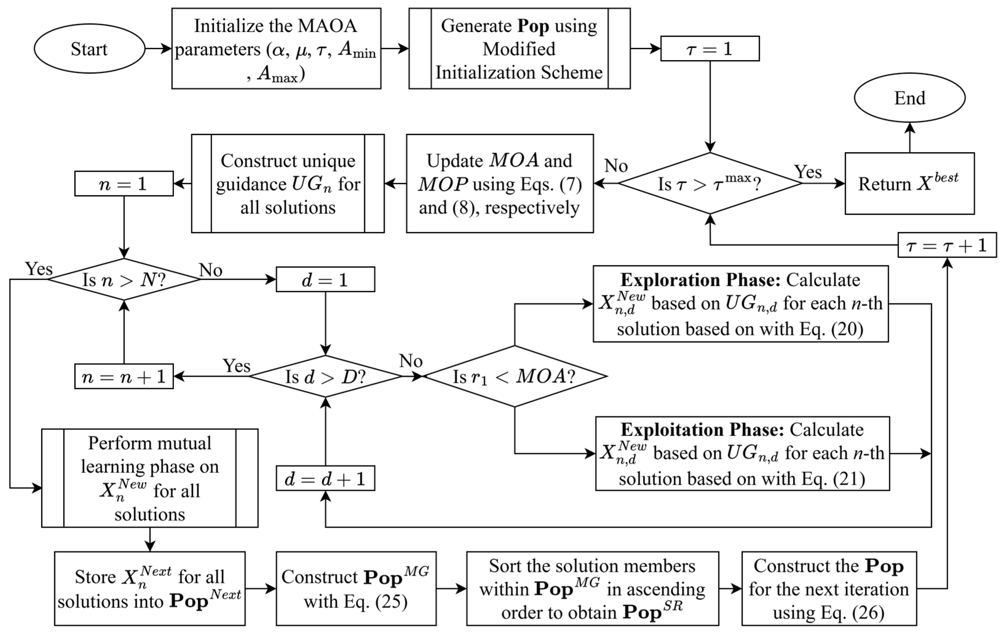
Figure 2 presents the flowchart of the modified initialization method used to create the initial population of MAOA. The first and second halves of the population created using the chaotic map and ROLM, respectively, are stored in the set variable P. The fitness value of each n-th solution in P is evaluated as f ( X n ) . For a minimization problem, a smaller value of f ( X n ) is desirable, whereas for a maximization problem, a larger value of f ( X n ) is preferred. The fitness evaluation process is repeated until all initial solutions in P are evaluated. The best-performing solution within the P is then identified, with its position vector and fitness value represented as X b e s t and f ( X b e s t ) , respectively.

3.2. Construction of Unique Guidance for MAOA

Upon carefully examining the four arithmetic operators of the original AOA, as shown in Equations (8) and (10), it is evident that all these four operators share a common attribute, i.e., the current best solution ( X b e s t ) is consistently used to guide and adjust the search trajectory of all solutions throughout the optimization process. While this approach may help to accelerate the converging nature of the original AOA during the early stages of optimization, the frequency of updating X b e s t tends to decrease in the middle or latter stages due to a loss of population diversity. In unfavorable scenarios where X b e s t becomes trapped in a local optimum early in the optimization process, especially when dealing with complex optimization problems featuring challenging fitness landscapes, the remaining solutions are likely to be misguided toward these suboptimal regions, resulting in premature convergence.
To handle the limitations encountered in the original AOA, the concept of unique guidance is introduced in the proposed MAOA. It is assumed that while X b e s t contains the most promising information at the current stage of optimization, it may not be ideal to use it as the sole guidance for all solutions due to the risk of premature convergence, particularly when dealing with complex optimization issues. Besides X b e s t , other well-performing solutions in the population also contain valuable information that can be utilized to guide the search process. Compared to using only X b e s t , leveraging multiple high-quality solutions to guide others is expected to direct the population toward promising regions while preserving population diversity. Motivated by this idea, the concept of unique guidance is incorporated into the proposed MAOA, enabling the search process of each solution to be influenced by a uniquely selected and well-performing guide. The mechanisms used to construct unique guidance for each solution in the MAOA population are detailed below.
During the iterative search process, the MAOA population is first sorted based on the fitness values of the solutions in descending order, i.e., from the worst to the best fitness values. In other words, the worse-performing solutions are assigned smaller population indices, while the better-performing solutions are assigned larger population indices. After completing the sorting process, a set variable Ψ n = { n , , N } is defined for each n-th solution having a population index of n = 1 , , N 1 to hold the population indices of other solutions that have better fitness values than the n-th solution. Evidently, the set Ψ n associated with the worse-performing solutions contains more elements compared to those associated with better-performing solutions.
Using the set Ψ n for each n-th solution, a better-performing solution is randomly selected from Ψ n to be used as unique guidance for adjusting the search trajectory of the n-th solution during optimization. Let κ n n , , N represent the population index of a better-performing solution randomly selected from Ψ n , and let U G n be the unique guidance assigned to the n-th solution. Then,
κ n = R a n d _ S e l e c t ( Ψ n = { n , , N } )
U G n = X κ n
where R a n d _ S e l e c t ( · ) is an operator used to randomly select an element from the given set Ψ n for each n-th solution.
It is noteworthy that Equations (14) and (15) are not applicable for the best-performing solution with the population index n = N because it has no other superior solution to serve as its unique guidance. In this case, a set variable Ψ N = { 1 , , N } is constructed for the best-performing N-th solution, enabling it to select any other solution from Ψ N as its unique guidance to explore wider regions of the solution space. Let κ N 1 , , N represent the population index of any solution randomly selected from Ψ N , and let U G N be the unique guidance assigned to the N-th solution. Then,
κ N = R a n d _ S e l e c t ( Ψ N = { 1 , , N } )
U G N = X κ N
The concept of unique guidance significantly enhances the resilience of MAOA to premature convergence by allowing each solution to perform a search under the influence of a distinct elite peer. In contrast to traditional global-best-based mechanisms, where all individuals are directed toward the same attractor, the unique guidance strategy promotes multi-attractor dynamics. Each solution is influenced by a superior individual selected from a personal set of better-performing peers, enabling diverse directional movement and preventing the entire population from collapsing into a narrow convergence cluster too early.
This behavioral shift is particularly beneficial when navigating complex fitness landscapes that contain multiple deceptive local optima. If all solutions are attracted to a single best solution X b e s t , and that solution resides in a suboptimal basin, the entire population may converge prematurely. However, under the unique guidance strategy, solutions are scattered across distinct regions, each influenced by different high-quality peers. This promotes competitive learning across niches, increases the diversity of search paths, and simultaneously maintains focus on high-potential regions. Additionally, even the best solution is exempt from rigid elitism, as it is guided by a randomly selected peer. This intentional disruption encourages continued exploration even among top individuals, helping to break the conventional greedy loop often observed in elitist metaheuristics.
From a technical standpoint, the unique guidance mechanism transforms the guidance model from a static, globally centralized structure into a stochastic dominance-based framework. Let Ψ n denote the set of solutions with better fitness than the n-th solution X n , such that Ψ n = N n , where the population is sorted in descending order, i.e., from the worst to the best fitness values. Since the best solution X b e s t (at population index N) is always a member of Ψ n , the probability that any X n selects X b e s t as its guide is as follows:
P g u i d e X n X b e s t = 1 Ψ n = 1 N n , f o r   n < N
This indicates that better-performing solutions (with larger indices n) have fewer options in Ψ n , and hence a higher probability of selecting X b e s t as their guide. On the other hand, the worse solutions (with smaller n) have access to a wider pool of elite guides, reducing the probability of following a single peer. This adaptive design reinforces exploitation among superior individuals while promoting exploration among weaker ones due to their access to greater guidance diversity.
For the best solution X N , which has no superior individuals, guidance is randomly selected from all other population members:
P g u i d e X N X k = 1 N 1 , f o r   k 1,2 , , N 1
This intentional randomness ensures that even the top solution participates in exploratory behavior, avoiding stagnation and reinforcing diversity at the elite level.
Let D ( t ) denote the average pairwise Euclidean distance between solutions at iteration t. In the original AOA, D ( t ) 0 rapidly as all solutions converge to X b e s t , leading to early stagnation. In contrast, the unique guidance strategy in MOAO preserves diversity such that D t > ϵ , where ϵ is a positive constant representing a minimal diversity threshold. This helps MAOA sustain search variation longer through early and mid-phases, increasing the likelihood of discovering latent optima through “late bloomers” in the population.
Furthermore, the proposed guidance strategy maintains population diversity across generations by preventing premature clustering around a single guide. It allows search trajectories to adapt dynamically based on fitness rank, reinforcing convergence in promising regions while ensuring broad exploration. This mechanism effectively replaces deterministic elitism with a probabilistic leadership model, allowing MAOA to strike a more effective and flexible balance between exploration and exploitation.
Figure 3 illustrates the flowchart used to derive the unique guidance ( U G n ) for each n-th solution, where n = 1 , , N , which is subsequently used to replace X b e s t in calculating the new position of each n-th solution during the exploration and exploitation phases. Let U G n , d represent the d-th dimension of the unique guidance assigned to the n-th solution. The d-th dimension of the new position vector for the n-th solution ( X n , d N e w ) is calculated during the exploration phase of MAOA (i.e., when r 1 < M O A ) as follows:
X n , d N e w = U G n , d ÷ M O P + χ × X d U X d L × 0.5 + X d L ,       if   r 2 < 0.5   U G n , d × M O P × X d U X d L × 0.5 + X d L ,                                   otherwise
During the exploitation phase of MAOA (i.e., when r 1 M O A ), the new position of the d-th dimension for the n-th solution X n , d N e w is calculated as follows:
X n , d N e w = U G n , d M O P × X d U X d L × 0.5 + X d L ,       if   r 3 < 0.5   U G n , d + M O P × X d U X d L × 0.5 + X d L ,       otherwise
Compared to the original AOA, the exploration and exploitation phases of MAOA, as defined in Equations (20) and (21), incorporate valuable information from other well-performing solutions beyond X b e s t offering a unique guidance scheme for each n-th learner. Since this unique guidance is derived from a subset of population members that are superior to the n-th learner, it is expected to provide effective guidance while still preserving population diversity.

3.3. Additional Learning Phase of MAOA

The unique guidance derived for each n-th solution in the previous subsection helps promote the population diversity of MAOA without compromising each solution’s ability to explore promising parts of the solution space. To enhance this process further, mutual learning is introduced as an additional learning phase in the proposed MAOA, enabling each new solution to interact with other solutions that may contain valuable information in certain dimensions. For each n-th solution, after obtaining the new solution in each d-th dimension, the mutual learning phase allows the new solution ( X n N e w ) to learn from another randomly selected solution in the original population. The mechanisms of the mutual learning phase in the proposed MAOA are described as follows.
Let Φ n = { 1 , n 1 , n + 1 , , N } represent a set containing the population indices of other solutions that the n-th learner can interact with during the mutual learning phase. The new solution X n N e w can interact with all other solutions except itself. During the mutual learning phase, the n-th solution randomly selects an element from Φ n to determine the population index of the solution it will interact with when updating the d-th component of its new solution ( X n , d N e w ), as follows:
γ n = R a n d _ S e l e c t ( Φ n = { 1 , n 1 , n + 1 , , N } )
M L n , d = X γ n , d
where M L n , d represents the d-th component of the mutual learner that interacts with the n-th solution for dimension d (i.e., X n , d N e w ). Notably, both Equations (22) and (23) are applied for D times to ensure that different dimensional components of a mutual learner can be contributed by different potential solutions from the original population.
Let X n , d N e x t represents the d-th component of the updated solution for the n-th solution after interacting with the mutual learner (i.e., M L n , d ), calculated as follows:
X n , d N e x t = X n , d N e w + r 5 ( M L n , d X n , d N e w )
The updated solutions for all population members of MAOA are generated by iteratively applying Equations (22)–(24) across all dimensions (i.e., d = 1 , , D ) for all solutions with population indices of n = 1 , , N . Figure 4 illustrates the mutual learning mechanism incorporated into the proposed MAOA.
The mutual learning phase serves as a crucial mechanism in MAOA to further sustain population diversity and mitigate stagnation risks, especially in the mid-to-late stages of the search process. While the unique guidance mechanism already promotes distributed learning by directing each individual toward a better peer, the additional learning phase introduces a second layer of interaction that facilitates decentralized knowledge diffusion. This form of structured interaction allows solutions to access complementary information from randomly selected peers, not necessarily limited to those superior in fitness. In doing so, MAOA avoids over-reliance on elite solutions and enables alternative paths to emerge, thus enhancing the algorithm’s resilience against deceptive local optima.
Most importantly, this mutual learning phase emulates a collaborative refinement strategy where partial solution components can evolve under the influence of different members of the population. Unlike conventional elitist-based updates that propagate dominant traits globally, this phase maintains diversity by decentralizing the influence map across the solution space. It effectively introduces a multi-source learning framework in which each dimension of a solution can be independently updated based on different references. This design fosters continual exploration and structural adaptability, which are crucial in complex or rotated landscapes where no single guide offers universal improvement. By doing so, MAOA ensures that even mediocre individuals are not prematurely excluded from the search process, providing late-blooming candidates a chance to emerge as high-quality solutions.
From a technical standpoint, the mutual learning phase introduces a fine-grained, dimension-level recombination scheme based on random peer selection. Recall that Φ n denotes the index set of all other individuals excluding the n-th solution. For each d-th dimension, the n-th solution selects a mutual learner with a population index of γ n Φ n and updates the d-th component of its new position X n , d N e w based on Equation (24). This means that each component of a solution may be influenced by a different peer, unlike conventional update rules that apply a uniform direction vector across all dimensions. Such cross-dimensional recombination promotes heterogeneous movement patterns, leading to higher inter-individual variability. As each component is drawn from a different landscape sample, the resulting solution has a higher probability of escaping local attractors. This randomized, dimension-wise inheritance reduces the likelihood of structural similarity in the population, thereby maintaining a higher average pairwise diversity D ( t ) across iterations.
Furthermore, the mutual learning process operates without introducing new control parameters or computational overhead, making it a lightweight yet powerful extension. Compared to techniques such as crossover in evolutionary algorithms or learning automata in particle-based methods, this approach avoids explicit combination weights or directional bias. It is thus less susceptible to premature convergence due to parameter misconfiguration. Instead, its randomness is functionally constrained, i.e., each dimension is updated using feasible and existing values from the population, thus preserving the feasibility and search-space consistency of the solution. This dual-level update process (unique guidance + mutual learning) gives MAOA a layered learning structure that adaptively shifts between directed convergence and stochastic recombination, ensuring a well-balanced trade-off between exploitation and exploration without compromising convergence speed.

3.4. Overall Workflow of MAOA

Figure 5 shows the flowchart used to explain the overall workflow of the proposed MAOA. Initially, the modified initialization scheme, as detailed in Figure 2, is used to generate the initial population of MAOA by harnessing the benefits offered by chaotic maps and ROLM. The MAOA population is represented as P = X 1 , , X n , , X N . During the iterative search process of MAOA, the construction mechanism described in Figure 3 is used to determine the unique guidance ( U G n ) assigned to each n-th solution to guide its search process. Unlike the original AOA, the U G n is used to calculate the new position ( X n , d N e w ) of each n-th solution in every d-th dimension using the four arithmetic operators, as described in Equations (20) and (21). After calculating the new position ( X n , d N e w ), mutual learning is further applied to each n-th solution based on the mechanism described in Figure 4 to calculate the d-th component of its updated position ( X n , d N e w ) by interacting with the corresponding dimension of the mutual learner ( M L n , d ). Fitness evaluation is then performed on the updated solution of each n-th solution to obtain the associated fitness value of f ( X n N e x t ) .
Let P N e x t = X 1 N e x t , , X n N e x t , , X N N e x t represent the set variable containing all updated solutions of MAOA produced through the mutual learning process. Both P = X 1 , , X n , , X N and P N e x t = X 1 N e x t , , X n N e x t , , X N N e x t are then combined to create a merged population ( P M G ) that has a population size of 2N, as follows:
P M G = P P N e x t
All solution members within P M G are then sorted based on their fitness values in ascending order, i.e., from the best to the worst fitness values, to generate a sorted population variable denoted as P S . In other words, the better-performing solutions in P S R are assigned smaller population indices, while the worse-performing solutions are assigned larger population indices. The best N solutions within P S R , having better fitness values, are then extracted to form the population P for the next iteration:
P = E x t r a c t ( P S R , N )
where E x t r a c t ( · , · ) is an operator that takes a population set and the number of elements to be selected from that set as the first and second input arguments, respectively. The iterative search process of MAOA is repeated until the termination count is attained, i.e., when the current iteration count ( τ ) exceeds the maximum number of iterations ( τ m a x ), i.e., τ > τ m a x .

3.5. Computational Complexity Analysis of MAOA

The computational complexity of the MAOA is analyzed using Big O notation to assess its scalability with respect to the population size N, dimensionality D, and maximum number of iterations τ m a x . The proposed MAOA integrates three major innovations over the original AOA, i.e., a modified initialization strategy using chaotic maps and ROLM, a unique guidance mechanism for solution update, and an additional mutual learning phase. Each component is carefully examined below.
The initialization phase of MAOA is divided into two stages, i.e., the first half of the population is generated using the circle chaotic map, and the second half is constructed via the ROLM. For each solution, the chaotic map requires Q internal iterations to compute chaotic variables before transforming them into positional values across D dimensions. Assuming Q is constant, the cost to initialize half the population is O ( N D ) . Similarly, ROLM operates over all D dimensions for the second half of the population, also incurring O ( N D ) . Thus, the total complexity for population initialization of MAOA is O ( N D ) .
The core iterative phase of MAOA consists of three nested operations, namely computing unique guidance, updating positions through exploration/exploitation arithmetic operators, and performing mutual learning. Each of these operations involves processing over all individuals and all dimensions.
In the unique guidance phase, the MAOA first sorts the population by fitness, which has a cost of O ( N log N ) . Then, for each solution, it creates a ranked set Ψ n , randomly samples a guide from Ψ n , and updates position based on guidance rules. This involves O ( N D ) operations per iteration. Hence, the guidance phase per iteration is O ( N log N + N D ) . During the solution update phase using arithmetic operators, the new position of each solution is calculated across all D dimensions, incorporating guidance from the selected peer. The arithmetic update operations involve simple expressions (addition, subtraction, multiplication, and division), which result in O ( N D ) per iteration.
The mutual learning phase allows each solution to independently update its dimensions by learning from a randomly selected peer solution. For each d-th dimension, the solution selects a random mutual, and the corresponding component is adopted based on Equation (24). This dimension-wise recombination is done for all N solutions, across all D dimensions, resulting in another O ( N D ) complexity per iteration.
Finally, after the new and original populations are merged, MAOA performs a sorting step on the merged population of size 2N, requiring O ( N log N ) times. The top N individuals are then selected for the next generation in constant time relative to sorting. Summarizing the total time complexity per iteration incurred by the sorting, guidance, position updates, and mutual learning, the total per-iteration complexity of MAOA becomes O ( N log N + N D ) . Considering the algorithm runs for τ m a x iterations, the overall computational complexity of MAOA becomes O ( τ m a x ( N log N + N D ) ) .
This expression shows that MAOA scales linearly with the number of dimensions D and the number of iterations τ m a x , and near-linearly with the population size N, aside from the log N term introduced by sorting. Notably, despite introducing multiple learning mechanisms, the algorithm avoids excessive overhead by keeping update operations lightweight and avoiding extra nested loops or parameter tuning routines. This makes MAOA computationally competitive and suitable for large-scale or high-dimensional optimization tasks.

4. Results and Discussion

The desired radiation characteristic of an electromagnetic problem is achieved by utilizing an LAA. Different optimization algorithms have been applied for the synthesis of these types of antenna arrays. In this section MAOA algorithm is proposed for optimizing the position and amplitude of the LAA elements. Here, the optimization goal is to synthesize an LAA having reduced PSLL, minimum CSLL, suppressed side lobes, and null positioning under the condition of fixed and variable beamwidth requirement by controlling the interelement spacing and current amplitude of the antenna elements separately. Eleven designs are showcased to compute the performance nature of the proposed algorithm, alongside a comparison with other prevalent intelligent optimization algorithms. The programming was carried out using MATLAB software (2024a) on a computer with an Intel Core i5 processor having 16 GB of RAM. The process was executed 15 times to obtain the desired optimized values. MAOA is a population-based iterative optimization algorithm; hence, the number of search agents and the iteration count are set to be 40 and 1000, respectively. Designs 1 to 5 illustrate that the position of the array elements is optimized, whereas designs 6 to 10 illustrate the amplitude-optimized LAA using the proposed algorithm. Design 11 showcases the amplitude-optimized CAA using the proposed algorithm.

4.1. Antenna Position Optimization

Optimizing the antenna position of an LAA plays a vital role in improving the signal quality, coverage area, system capacity, energy efficiency, and cost reduction. Therefore, the positions ( x n ) are determined using the MAOA algorithm considering the uniform current amplitudes ( I n = 1) and phase ( Ø n = 0) for n = 1 to N, and the comparison has been made with other intelligent metaheuristic optimization algorithms. The spacing between the elements of the antenna ranges from 0.25 λ to 0.50 λ . The array factor for position optimization is mentioned in Equation (3). In designs 1 and 2, the positions of the array elements are optimized for PSLL reduction and CSLL minimization, respectively, while side lobe power minimization without any condition on FNBW is discussed in design 3. Side lobe suppression with null positioning is discussed in design 4, whereas design 5 illustrates the side lobe average power minimization with a fixed FNBW constraint.

4.1.1. Design 1: Peak Side Lobe Level Minimization of a 10-Element LAA

The MAOA algorithm is applied to estimate the position of all the antenna elements from the origin. The fitness function for this design is provided in Equation (27), where θ represents the region of the side lobes. In this equation, max 20 log A F θ provides the maximum SLL called PSLL, and AF(θ) denotes the array factor given in Equation (3). The antenna position has been optimized for minimizing the PSLL in the region θ = [ 0 ° , 74 ° ] and θ = [ 106 ° , 180 ° ].
f i t n e s s   f u n c t i o n = m i n m a x 20 log A F θ m a x A F θ
The number of antenna elements is even; hence, to make a symmetrical layout of the array, no elements are placed at the origin. The results are shown in Table 1, highlighting PSLL and the optimized positions of the right-sided five array elements from the origin expressed as a multiple of λ . The left-sided elements have the same position from the origin on the opposite side. The mentioned PSLL indicates that MAOA provides considerable PSLL minimization from −12.97 to −21.82 dB, i.e., a reduction of 8.85 dB from conventional ULA. Similarly, a reduction of 2.1 dB from PSO, 0.51 dB from GOA, and 1.57 dB from SMO-optimized antenna array is observed. The array pattern obtained using the optimized position is illustrated in Figure 6.

4.1.2. Design 2: Close-In Side Lobe Level Minimization of a 10-Element LAA

For minimizing the CSLL (Side lobe adjacent to main lobe), the antenna position is optimized using the MAOA optimization algorithm. The fitness function for this design is provided in Equation (28), where θ A S represents the total region of the side lobes, while θ N S is the region of close-in side lobes. The weight factors w 1 and w 2 add more degrees of freedom to design a sophisticated antenna system. In this design, θ A S = [ 0 ° , 76 ° ] and [ 104 ° , 180 ° ] and θ N S = [ 69 ° , 76 ° ] and [ 104 ° , 111 ° ] are the values decided for the fitness function, and both weight factors are taken to be unity.
f i t n e s s   f u n c t i o n = m i n w 1 m a x 20 log A F θ A S + w 2 m a x 20 log A F θ N S
The simulation results are mentioned in Table 2, highlighting the optimized element positions along with the CSLL. The highest reduction of −34.50 dB in the near side lobe is attained with MAOA. The result is benchmarked with other nature-inspired optimization algorithms and shows a reduction of 21.53 dB from conventional ULA, 4.26 dB from ALO, 3.50 dB from PSO, and 3.20 dB from GWO-optimized antenna array. The array pattern for this design is illustrated in Figure 7.

4.1.3. Design 3: Side Lobe Average Power Minimization Without FNBW Constraint of a 20-Element LAA

The total side lobe average power minimization of an LAA with no constraints on FNBW is focused here by optimizing the position parameter using the MAOA algorithm. The fitness function for this design is provided in Equation (29), which requires an integration of the array factor. In this equation, θ l i and θ u i are the lower and upper bounds of the region in which the SLL is required to be suppressed, while θ i = [ θ u i θ l i ] is the difference between them. The values of the SLL region focused on for minimization are [ 0 ° , 82 ° ] and [ 98 ° , 180 ° ].
f i t n e s s   f u n c t i o n = i 1 θ i θ l i θ u i A F θ 2 d θ
The fitness function is simulated by using three optimization algorithms, and the obtained values of the positions are listed in Table 3. The array pattern using these optimized position values is shown in Figure 8, and Table 4 indicates the SLL of the 20-element LAA along with the FNBW obtained by ULA, ALO, AOA, and MAOA. The average power for one-half SLL of ULA is −21.68 dB, which is now reduced to −25.75 dB by MAOA, offering an improvement of 4.07 dB of average SLL power in this design by using the proposed algorithm.

4.1.4. Design 4: Side Lobe Average Power Minimization Along with Null Placement of a 20-Element LAA

The deep null placement, along with the SLL reduction, is presented in this design by controlling the position of the antenna elements. The fitness function used in this design is provided in Equation (30), where the first part deals with SLL reduction, while the latter is responsible for placing the nulls at appropriate locations as defined by θ k . Here, the region of the side lobes is considered as [ 0 ° , 82 ° ] and [ 98 ° , 180 ° ], while the nulls are required at 64 ° , 76 ° , 104 ° , and 116 ° .
f i t n e s s   f u n c t i o n = i 1 θ i θ l i θ u i A F θ 2 d θ + k A F θ k 2
The optimized antenna positions obtained after simulation are mentioned in Table 5, while the array pattern is outlined in Figure 9. The null depth level in decibels and FNBW in degrees are outlined in Table 6. This clearly indicates that maximum null depths of −64.21 dB and −89.00 dB are attained with MAOA in comparison to ALO, AOA, and DA-optimized antenna arrays. The beamwidth with MAOA is increased by 4.20 dB from ULA but is still less broadening in comparison to other applied algorithms.

4.1.5. Design 5: Side Lobe Average Power Minimization Along with FNBW Constraint of a 20-Element LAA

This multi-objective function is handled by optimizing the position of the antenna elements using MAOA. The fitness function for this design is provided in Equation (31), where SLL reduction is governed by the first part, whereas the second part focuses on maintaining the constant beamwidth offered by the antenna array. In this design, the side lobe region is decided as [ 0 ° , 82 ° ] and [ 98 ° , 180 ° ].
f i t n e s s   f u n c t i o n = w 1 i 1 θ i θ l i θ u i A F θ 2 d θ + w 2 F N B W C o m p u t e d F N B W I n = 1
Table 7 summarizes the location of the various elements of the antenna array obtained by applying the ALO, DA, sooty tern optimization (STO), and MAOA optimization algorithms, along with the FNBW offered by different algorithms. The array pattern is showcased in Figure 10, whose outcome reveals that MAOA reduces the SLL of the antenna array more efficiently and offers a comparatively constant FNBW of 11.60 degrees. Figure 11 depicts the convergence plot of different optimization algorithms for attaining the position of antenna elements, and the result shows that the proposed MAOA has a good rate of convergence in comparison to other optimization algorithms.

4.2. Antenna Current Amplitude Optimization

To optimize the current amplitude of the antenna elements in an LAA, the following assumptions are made for the other two parameters. The phase is assumed to be constant, i.e., ϕ n = 0, and the array elements are placed at equal distances from each other with x n = n × (λ/2), where n = −N to N. Using these two conditions, the array factor used for current amplitude optimization is provided in Equation (5). The magnitude of the excitation current amplitude lies between 0 and 1. Five designs of LAA are optimized using MAOA along with other intelligent optimization algorithms for comparison purposes. In designs 6 and 7, the current amplitude of the array elements is considered for optimization, respectively, for reducing PSLL and CSLL minimization, while side lobe average power minimization without any condition on FNBW is discussed in design 8. Side lobe suppression with null positioning is discussed in design 9, whereas design 10 illustrates the side lobe average power minimization with a fixed FNBW constraint.

4.2.1. Design 6: Peak Side Lobe Level Minimization of a 10-Element LAA

The fitness function used to minimize the PSLL of an LAA is mentioned in Equation (25). The antenna current amplitude has been optimized for minimizing the PSLL in the region θ = [ 0 ° , 74 ° ] and θ = [ 106 ° , 180 ° ]. The MAOA and other metaheuristic algorithms are applied to compute these optimized amplitudes. The simulation results are shown in Table 8, highlighting PSLL and the optimized current amplitude of the right-sided five array elements. In this design, the number of antenna elements is even; hence, for making a symmetrical array, no element is placed at the origin. The simulation outcome indicates that MAOA provides considerable PSLL minimization from −12.97 dB to −24.32 dB, as compared to the conventional ULA, offering a reduction of 11.35 dB. Also, in comparison with other algorithms, MAOA offers a reduction in PSLL of 0.86 dB with DA, 0.03 dB with STO, and 6.57 dB with dung beetle optimization (DBO) optimized antenna array. The array pattern is highlighted in Figure 12. The converging nature of all the algorithms is highlighted in Figure 13, which suggests that MAOA optimizes the current amplitude in less time compared with other optimization algorithms.

4.2.2. Design 7: Close-In Side Lobe Level Minimization of a 10-Element LAA

In this design, the close-in side lobe levels are minimized using the MAOA optimization algorithm. The fitness function for this design is showcased in Equation (26), where θ A S is the total region of the side lobes, θ N S is the region of close-in side lobes, and w 1 , w 2 are the weight factors. In this design, θ A S = [ 0 ° , 76 ° ] and [ 104 ° , 180 ° ] and θ N S = [ 69 ° , 76 ° ] and [ 104 ° , 111 ° ] are the two regions decided for the fitness function, and both the weight factors are taken to be unity.
The results of the simulation are mentioned in Table 9, highlighting the optimized current amplitude along with the CSLL in decibels. The highest reduction of −29.79 dB in the near side lobe is attained with MAOA. The result is benchmarked with other nature-inspired optimization algorithms, and MAOA provides a PSLL reduction of 16.82 dB from conventional ULA and also less than AOA, DA, and BBO optimized antenna arrays. The array pattern is illustrated in Figure 14.

4.2.3. Design 8: Side Lobe Average Power Minimization Without FNBW Constraint of a 20-Element LAA

The MAOA algorithm is considered to optimize the current amplitude of a 20-element LAA to reduce the SLL average power. The SLL region focused here for minimization is [ 0 ° , 82 ° ] and [ 98 ° , 180 ° ]. For this design, the fitness function is illustrated above in Equation (27), which requires an integration of the array factor. The normalized current amplitude obtained after simulation is outlined in Table 10. These amplitudes help in plotting the array factor of the antenna array as showcased in Figure 15. Analysis of the array factor clearly demonstrates that the SLL average power is reduced drastically in this design by MAOA in comparison to ULA, AOA, and STO optimized antenna arrays. Comparison of the SLL and FNBW is outlined in Table 11. The SLL power and the FNBW are interrelated parameters—reducing SLL affects the beamwidth and vice versa.

4.2.4. Design 9: Side Lobe Average Power Minimization Along with Null Placement of a 20-Element LAA

The SLL average power minimization with deep placement of the nulls is considered in this design by adjusting the current amplitude of the antenna elements. The fitness function applicable for this design is illustrated above in Equation (28), in which the first part deals with SLL average power minimization, and the second is responsible for placing the deeper nulls at appropriate locations as defined by θ k . Here, the region of the side lobes is decided as [ 0 ° , 82 ° ] and [ 98 ° , 180 ° ], and the nulls are required at 64 ° , 76 ° , 104 ° , and 116 ° . The MAOA, ALO, AOA, and STO algorithms are used here to optimize the current amplitude of the LAA, and the values thus obtained are mentioned in Table 12. Using these values of the current amplitude, the array pattern is drawn as mentioned in Figure 16. Comparison of the null depth and FNBW is outlined in Table 13. Consistent null depths are obtained at the four required locations by MAOA, whereas other algorithms provide better null depth at some locations but worse at the other locations of the required nulls. Figure 17 depicts the convergence profile of different algorithms, and the graph shows that the proposed algorithm presents comparable results in comparison to other algorithms.

4.2.5. Design 10: Side Lobe Average Power Minimization Along with FNBW Constraint of a 20-Element LAA

In this design, SLL reduction of a 20-element LAA is performed with the condition that the beamwidth remains unchanged. To handle these two objectives simultaneously, the fitness function is formulated and mentioned above in Equation (29). The current amplitude is then optimized for the reduction of SLL in the region [ 0 ° , 82 ° ] and [ 98 ° , 180 ° ]. The normalized current amplitude and FNBW obtained after simulation of the fitness function by various optimization algorithms are outlined in Table 14, and the array pattern is illustrated in Figure 18. The outcome reveals that MAOA not only minimizes the average power of the SLL but also maintains the constant beamwidth of the antenna array taken into consideration. The FNBW offered by ULA is 11.40 degrees, while by MAOA, it is 10.80 degrees; hence, almost constant beamwidth is offered by the proposed optimization algorithm. Figure 19 presents the convergence profile of different algorithms, and the profile shows that the proposed algorithm presents comparable results. Therefore, the MAOA algorithm is superior to other applied optimization algorithms in optimizing the current amplitude and improving the antenna array radiation performance.

4.3. Circular Antenna Array

CAA is one of the most commonly used antenna array configurations in radar and mobile communication applications because of its adaptive beamforming and direction-finding capabilities. In this configuration, the elements are placed in a circular configuration as shown in Figure 20.
The array factor of CAA is given by
A F ( Φ , I , d ) = i = 1 N I n e x p ( j [ k a sin θ . cos ( Φ Φ n ) + α n ] )
k a = 2 π a λ = i = 1 N d i λ   a n d   Φ n = 2 π i = 1 N d i k a = 2 π n N
where I n denotes the excitation current of the n-th element in the antenna array. The distance between the i-th and (i + 1)-th elements is represented by d i , and a represents the radius of the circle. The wave number k is defined as k = 2 π λ , where λ is the wavelength of operation. The elevation angle, measured from the z-axis, is denoted by θ , while Φ represents the azimuth angle measured from the x-axis. The angular position of the n-th element in the x-y plane is given by Φ n , and its phase excitation is α n . The total number of elements in the CAA is denoted by N.

Design 11: SLL Reduction with FNBW Constraint of a 14-Element CAA

The fitness function for this multi-objective goal is given in (33), in which the FNBW constraint is handled by the first term, while the second is responsible for the reduction in SLL of the CAA,
f i t n e s s = w 1 × A F θ n u 1 + A F θ n u 2 + w 2 × A F θ m s k 1 + A F θ m s k 2
θ n u 1 and θ n u 2 represents the lower and upper nulls of the main beam, respectively, while θ m s k 1 and θ m s k 2 denotes the angle of the maximum side lobe in the lower region π   t o   θ n u 1 and upper region θ n u 2   t o   π respectively. w 1 and w 2 are the weighting factors for the above two objectives, which add more flexibility in tuning the two constraints. In this case, their values are w 1 = 0.1 and w 2 = 0.9.
This design highlights the synthesis of 14-element CAA for minimizing the SLL along with constant beamwidth. Here, the parameter selected for optimization is the excitation amplitude of the individual antenna elements. The goal here is to obtain a radiation pattern having SLL less than the uniform CAA, which is −5.50 dB, along with a constant beamwidth of 39.26 ° , which is the beamwidth of the uniform circular array (UCA). MAOA is applied to estimate the non-uniform amplitudes of the CAA for which the simulation is performed with 15 independent runs having 1000 iterations in each run. The lower bound limit is 0.1, while the upper bound has a value of 1. The obtained radiation pattern is shown in Figure 21. The MAOA provides an SLL of −6.85 dB with a beamwidth of 47.92 ° , while PSO provides an SLL of −6.07 dB with a beamwidth of 49.48 ° . Hence, MAOA optimized CAA offers a better SLL reduction and constant beamwidth than the UCA and PSO optimized antenna arrays.

4.4. Full Wave Analysis Using EM Simulator

In this section, the simulation results of design 6 are verified through full-wave electromagnetic simulation using the commercially available EM solver CST Microwave Studio. The optimized amplitude obtained using different metaheuristic algorithms in design 6 for PSLL minimization and presented in Table 8 are taken as input to simulate a 10-element inset-feed patch antenna array in the EM simulator. The dimensions of the patch antenna are presented in Figure 22 and Figure 23 shows the geometrical representation of the antenna array.
Figure 24 displays the normalized array pattern with respect to the azimuthal angle for ULA, DA, STO, DBO, and the proposed MAOA. The simulation results indicate that there is a strong agreement between the radiation characteristics obtained using the EM simulator and the MATLAB software. The proposed MAOA presents the lowest PSLL in comparison to other optimization algorithms and finds applications in wireless applications.

4.5. Statistical Validation

The Wilcoxon rank sum test [33] is applied for estimating the level of difference in two independent samples, this then used here to analyze the authenticity of the proposed MAOA. Here, the optimization algorithm is carried out for 15 independent runs with 1000 iteration on each run, using this test the performance of the proposed algorithm is analyzed as compared to other applied algorithms. The level of significance to perform this test is decided as 5%. The outcome of the test for the ten different designs of LAA has been outlined in Table 15. The outcome of this analysis reveals that MAOA algorithm outperforms the other intelligent optimization algorithms (ALO, AOA, PSO, GWO, GOA, SMO, BBO, DA, STO, and DBO). In most cases, higher R+ values are provided by MAOA indicating its superior performance over the other algorithm. In some cases, R- is higher for MAOA, but in overall comparison MAOA provides better optimal values of position and current amplitude than other algorithms. Figure 25 and Figure 26 show the results of Friedman ranking tests for all the optimization algorithms across all ten designs of LAA with an overall confidence level of 95%. The results show that the proposed MAOA presents good ranking in most of the designs which signifies its suitability in optimizing the complex electromagnetic problems and are thus immerge as effective tool for performing the antenna array pattern synthesis.

5. Conclusions

In this paper, a modified optimization algorithm known as MAOA is implemented for solving the problem of antenna array pattern synthesis with different objectives. The proposed algorithm efficiently handles the problem and, in turn, generates the optimal values of position and current amplitude for various designs of an LAA. High performance level is offered in PSLL reduction, CSLL minimization, SLL minimization with and without beamwidth constraint also helps in controlling the direction of the nulls. The result thus obtained is benchmarked with other well-known intelligent optimization algorithms, and MAOA outperforms in every aspect for synthesizing the LAA of different designs. One design of CAA is also considered in this research, and the simulation result shows that MAOA-optimized array outperforms UCA and PSO-optimized antenna array. The simulation results reveal that MAOA handles the optimization problem of the antenna array in a much convenient manner and can also be applied for any electromagnetic engineering problem. In addition to this, a statistical test called Wilcoxon rank sum test and Friedman rank are also performed for checking the authenticity of the proposed algorithm, the test results also point that MAOA is an efficient technique for the said problem of pattern synthesis. Based on its performance, this algorithm equally applied to synthesize other antenna geometries like concentric, elliptical, planar, and conformal antenna arrays.

Author Contributions

Conceptualization, A.R., A.S. (Abhinav Sharma) and W.H.L.; methodology, A.S. (Abhinav Sharma), A.S. (Abhishek Sharma), A.K.A., R.S. and W.H.L.; simulation, A.R. and A.S. (Abhinav Sharma); validation, A.R. and A.K.A.; formal analysis, A.R. and W.H.L.; investigation, A.R. and A.S. (Abhinav Sharma); resources, W.H.L. and A.S. (Abhinav Sharma); data curation, A.R., K.S.C. and S.S.T.; writing—original draft preparation, A.R.; writing—review and editing, A.S. (Abhinav Sharma), W.H.L., K.S.C. and S.S.T.; visualization, A.R. and R.S.; supervision, A.S. (Abhinav Sharma); project administration, A.S. (Abhinav Sharma); funding acquisition, K.S.C., S.S.T. and W.H.L. All authors have read and agreed to the published version of the manuscript.

Funding

The study was funded by the Malaysian Ministry of Higher Education through the Fundamental Research Grant Scheme (FRGS/1/2024/TK07/UCSI/02/1).

Data Availability Statement

Data are contained within the article.

Conflicts of Interest

Author Abhishek Kumar Awasthi was employed by the company Paras Antidrone Technologies Private Limited. The remaining authors declare that the research was conducted in the absence of any commercial or financial relationships that could be construed as a potential conflict of interest.

Abbreviations

ALOAnt lion optimization
BBOBiogeography-based optimization
CSLLClose-in side lobe level
CAACircular antenna array
DADragonfly optimization
dBDecibels
DBODung beetle optimization
FNBWFirst null beamwidth
GBGigabyte
GOAGrasshopper optimization algorithm
GWOGrey wolf optimization
LAALinear antenna array
MAOAModified arithmetic optimization algorithm
MATLABMatrix laboratory
MOAMath optimizer accelerated
MOPMath optimizer probability
PSLLPeak side lobe level
PSOParticle swarm optimization
RAMRandom access memory
ROLMRandom oppositional-based learning mechanism
SLLSide lobe level
SMOSpider monkey optimization
STOSooty tern optimization
UCAUniform circular array
ULAUniform linear array

References

  1. Sharma, A. Antenna array pattern synthesis using metaheuristic algorithm: A review. IETE Tech. Rev. 2022, 40, 90–115. [Google Scholar] [CrossRef]
  2. Pappula, L.; Ghosh, D. Linear antenna array synthesis using cat swarm optimization. AEU—Int. J. Electron. Commun. 2014, 68, 540–549. [Google Scholar] [CrossRef]
  3. Wang, H.; Liu, C.; Wu, H.; Li, B.; Xie, X. Optimal Pattern Synthesis of Linear Array and Broadband Design of Whip Antenna Using Grasshopper Optimization Algorithm. Int. J. Antennas Propag. 2020, 1, 5904018. [Google Scholar] [CrossRef]
  4. Khodier, M.; Aqeel, M.A. Linear and circular array optimization: A study using particle swarm intelligence. Prog. Electromagn. Res. B 2009, 15, 347–373. [Google Scholar] [CrossRef]
  5. Sharma, A.; Mathur, S. A novel adaptive beamforming with reduced side lobe level using GSA. COMPEL-Int. J. Comput. Math. Electr. Electron. Eng. 2018, 37, 2263–2278. [Google Scholar] [CrossRef]
  6. Raghuvanshi, A.; Sharma, A.; Gupta, M.K. Maximum Likelihood Direction of Arrival Estimation using GWO Algorithm. In Proceedings of the International Conference on Advances in Computing, Communication and Materials, ICACCM, Dehradun, India, 10–11 November 2022. [Google Scholar]
  7. Guney, K.; Basbug, S. A quantized water cycle optimization algorithm for antenna array synthesis by using digital phase shifters. Int. J. RF Microw. Comput.-Aided Eng. 2015, 25, 21–29. [Google Scholar] [CrossRef]
  8. Pelosi, G.; Selleri, S.; Taddei, R. A novel multiobjective taguchi’s optimization technique for multibeam array synthesis. Microw. Opt. Technol. Lett. 2013, 55, 1836–1840. [Google Scholar] [CrossRef]
  9. Zhang, R.; Zhang, Y.; Sun, J.; Li, Q. Pattern synthesis of linear antenna array using improved differential evolution algorithm with sps framework. Sensors 2020, 20, 5158. [Google Scholar] [CrossRef]
  10. Das, A.; Mandal, D.; Kar, R. An optimal compact time-modulated circular antenna array synthesis using krill herd optimization. Ann. Telecommun. 2021, 76, 467–482. [Google Scholar] [CrossRef]
  11. Kumar, S.; Singh, H. Antenna array pattern synthesis using nature-inspired computational techniques: A review. Arch. Comput. Methods Eng. 2023, 30, 3235–3269. [Google Scholar] [CrossRef]
  12. Lakhlef, N.; Oudira, H.; Dumond, C. Optimal Pattern Synthesis of Linear Antenna Arrays Using Modified Grey Wolf Optimization Algorithm. Instrum. Mes. Métrologie 2020, 19, 255–261. [Google Scholar] [CrossRef]
  13. Pavani, T.; Padmavathi, K.; Kumari, C.U.; Ushasree, A. Design of array antennas via atom search optimization. Mater. Today Proc. 2023, 80, 2051–2054. [Google Scholar] [CrossRef]
  14. Almagboul, M.A.; Shu, F.; Qian, Y.; Zhou, X.; Wang, J.; Hu, J. Atom search optimization algorithm-based hybrid antenna array receive beamforming to control sidelobe level and steering the null. AEU—Int. J. Electron. Commun. 2019, 111, 152854. [Google Scholar] [CrossRef]
  15. Grewal, N.S.; Rattan, M.; Patterh, M.S. A linear antenna array failure correction using improved bat algorithm. Int. J. RF Microw. Comput.-Aided Eng. 2017, 27, e21119. [Google Scholar] [CrossRef]
  16. Das, A.; Mandal, D.; Ghoshal, S.P.; Kar, R. An efficient side lobe reduction technique considering mutual coupling effect in linear array antenna using BAT algorithm. Swarm Evol. Comput. 2017, 35, 26–40. [Google Scholar] [CrossRef]
  17. Guney, K.; Basbug, S. Interference suppression of linear antenna arrays by amplitude-only control using a bacterial foraging algorithm. Prog. Electromagn. Res. 2008, 49, 475–497. [Google Scholar] [CrossRef]
  18. Ram, G.; Mandal, D.; Kar, R.; Ghoshal, S.P. Circular and Concentric Circular Antenna Array Synthesis Using Cat Swarm Optimization. IETE Tech. Rev. 2015, 32, 204–217. [Google Scholar] [CrossRef]
  19. Pappula, L.; Ghosh, D. Synthesis of linear aperiodic array using Cauchy mutated cat swarm optimization. AEU—Int. J. Electron. Commun. 2017, 72, 52–64. [Google Scholar] [CrossRef]
  20. Babayigit, B. Synthesis of concentric circular antenna arrays using dragonfly algorithm. Int. J. Electron. 2018, 105, 784–793. [Google Scholar] [CrossRef]
  21. Saxena, P.; Kothari, A. Linear antenna array optimization using flower pollination algorithm. Springerplus 2016, 5, 306. [Google Scholar] [CrossRef]
  22. Saxena, P.; Kothari, A. Optimal Pattern Synthesis of Linear Antenna Array Using Grey Wolf Optimization Algorithm. Int. J. Antennas Propag. 2016, 1, 1205970. [Google Scholar] [CrossRef]
  23. Das, A.; Mandal, D.; Ghoshal, S.P.; Kar, R. Moth flame optimization-based design of linear and circular antenna array for side lobe reduction. Int. J. Numer. Model. 2019, 32, e2486. [Google Scholar] [CrossRef]
  24. Bataineh, M.H.; Ababneh, J.I. Synthesis of aperiodic linear phased antenna arrays using particle swarm optimization. Electromagnetics 2006, 26, 531–541. [Google Scholar] [CrossRef]
  25. Swathi, A.V.S.; Chakravarthy, V.V.S.S.S.; Krishna, M.V. Circular antenna array optimization using modified social group optimization algorithm. Soft Comput. 2021, 25, 10467–10475. [Google Scholar] [CrossRef]
  26. Weng, W.C.; Yang, F.; Elsherbeni, A.Z. Linear antenna array synthesis using Taguchi’s method: A novel optimization technique in electromagnetics. IEEE Trans. Antennas Propag. 2007, 55, 723–730. [Google Scholar] [CrossRef]
  27. Singh, U.; Kumar, H.; Kamal, T.S. Linear array synthesis using biogeography based optimization. Prog. Electromagn. Res. M 2010, 11, 25–36. [Google Scholar] [CrossRef]
  28. Saxena, P.; Kothari, A. Ant Lion Optimization algorithm to control side lobe level and null depths in linear antenna arrays. AEU-Int. J. Electron. Commun. 2016, 70, 1339–1349. [Google Scholar] [CrossRef]
  29. Al-Azza, A.A.; Al-Jodah, A.A.; Harackiewicz, F.J. Spider Monkey Optimization: A Novel Technique for Antenna Optimization. IEEE Antennas Wirel. Propag. Lett. 2016, 15, 1016–1019. [Google Scholar] [CrossRef]
  30. Das, A.; Mandal, D.; Kar, R. An optimal far-field radiation pattern synthesis of time-modulated linear and concentric circular antenna array. Int. J. Numer. Model. 2019, 32, e2658. [Google Scholar] [CrossRef]
  31. Prabhakar, D.; Satyanarayana, M. Side lobe pattern synthesis using hybrid SSWOA algorithm for conformal antenna array. Eng. Sci. Technol. Int. J. 2019, 22, 1169–1174. [Google Scholar] [CrossRef]
  32. Ram, G.; Mandal, D.; Kar, R.; Ghoshal, S.P. Radiation Performance Characteristic Optimization of Time-Modulated Circular Antenna Arrays. IETE Tech. Rev. 2017, 35, 190–204. [Google Scholar] [CrossRef]
  33. Derrac, J.; García, S.; Molina, D.; Herrera, F. A practical tutorial on the use of nonparametric statistical tests as a methodology for comparing evolutionary and swarm intelligence algorithms. Swarm Evol. Comput. 2011, 1, 3–18. [Google Scholar] [CrossRef]
  34. Abualigah, L.; Diabat, A.; Mirjalili, S.; Elaziz, M.A.; Gandomi, A.H. The Arithmetic Optimization Algorithm. Comput. Methods Appl. Mech. Eng. 2021, 376, 113609. [Google Scholar] [CrossRef]
  35. Kaveh, A.; Hamedani, K.B. Improved arithmetic optimization algorithm and its application to discrete structural optimization. Structures 2022, 35, 748–764. [Google Scholar] [CrossRef]
  36. Fang, H.; Fu, X.; Zeng, Z.; Zhong, K.; Liu, S. An Improved Arithmetic Optimization Algorithm and Its Application to Determine the Parameters of Support Vector Machine. Mathematics 2022, 10, 2875. [Google Scholar] [CrossRef]
  37. Khatir, S.; Tiachacht, S.; Thanh, C.L.; Ghandourah, E.; Mirjalili, S.; Wahab, M.A. An improved Artificial Neural Network using Arithmetic Optimization Algorithm for damage assessment in FGM composite plates. Compos. Struct. 2021, 273, 114287. [Google Scholar] [CrossRef]
  38. Mohamed, M.A.E.; Ahmed, S.N.; Metwally, M.E. Arithmetic optimization algorithm based maximum power point tracking for grid-connected photovoltaic system. Sci. Rep. 2023, 13, 5961. [Google Scholar] [CrossRef]
  39. Khodadadi, N.; Khodadadi, E.; Tashi, Q.A.; Kenawy, E.E.; Abualigah, L.; Abdulkadir, S.J.; Alqushaibi, A.; Mirjalili, S. BAOA: Binary Arithmetic Optimization Algorithm With K-Nearest Neighbor Classifier for Feature Selection. IEEE Access 2023, 11, 94094–94115. [Google Scholar] [CrossRef]
Figure 1. LAA with 2N elements distributed horizontally on the x-axis.
Telecom 06 00034 g001
Figure 2. Flowchart of the modified initialization method for the proposed MAOA.
Telecom 06 00034 g002
Figure 3. Flowchart for constructing unique guidance in MAOA.
Telecom 06 00034 g003
Figure 4. Flowchart illustrating the mutual learning phase in MAOA.
Telecom 06 00034 g004
Figure 5. Flowchart of the MAOA algorithm.
Telecom 06 00034 g005
Figure 6. Array pattern of a 10-element LAA for design 1.
Telecom 06 00034 g006
Figure 7. Array pattern of a 10-element LAA for design 2.
Telecom 06 00034 g007
Figure 8. Array pattern of a 20-element LAA for design 3.
Telecom 06 00034 g008
Figure 9. Array pattern of a 20-element LAA for design 4.
Telecom 06 00034 g009
Figure 10. Array pattern of a 20-element LAA for design 5.
Telecom 06 00034 g010
Figure 11. Convergence profile of design 5.
Telecom 06 00034 g011
Figure 12. Array pattern of a 10-element LAA for design 6.
Telecom 06 00034 g012
Figure 13. Convergence profile of design 6.
Telecom 06 00034 g013
Figure 14. Array pattern of a 10-element LAA for design 7.
Telecom 06 00034 g014
Figure 15. Array pattern of a 20-element LAA for design 8.
Telecom 06 00034 g015
Figure 16. Array pattern of a 20-element LAA for design 9.
Telecom 06 00034 g016
Figure 17. Convergence profile of design 9.
Telecom 06 00034 g017
Figure 18. Array pattern of a 20-element LAA for design 10.
Telecom 06 00034 g018
Figure 19. Convergence profile of design 10.
Telecom 06 00034 g019
Figure 20. Geometry of a circular antenna array having N antenna elements.
Telecom 06 00034 g020
Figure 21. Array pattern of a 14-element CAA for design 11.
Telecom 06 00034 g021
Figure 22. Inset Feed Patch Antenna.
Telecom 06 00034 g022
Figure 23. Inset Feed Patch Linear Antenna Array.
Telecom 06 00034 g023
Figure 24. Normalized Array Pattern of design 6 in EM Simulator.
Telecom 06 00034 g024
Figure 25. Friedman ranking of optimization algorithms used for position optimization of LAA.
Telecom 06 00034 g025
Figure 26. Friedman ranking of optimization algorithms used for amplitude optimization of LAA.
Telecom 06 00034 g026
Table 1. Optimized positions for positive half elements and PSLL of design 1.
Method Optimized   Element   Positions   (×λ)PSLL (dB)
IIIIIIIVV
ULA0.25000.75001.25001.75002.2500−12.97
PSO [4]0.21460.59991.06111.58702.2500−19.72
GOA [3]0.33600.41961.01261.41662.1000−21.31
SMO [29]0.23600.52801.00701.47102.1260−20.25
MAOA0.20470.40720.82841.16761.7464−21.82
Table 2. Optimized positions for positive half elements and CSLL of design 2.
Method Optimized   Element   Positions   (×λ)CSLL (dB)
IIIIIIIVV
ULA0.25000.75001.25001.75002.2500−12.97
ALO [28]0.17920.54070.94521.50972.2500−30.24
PSO [4]0.16850.54610.93641.51072.2500−31.00
GWO [22]0.17920.54100.93541.50962.2500−31.30
MAOA0.16690.54430.83211.47392.1409−34.50
Table 3. Optimized positions for positive half elements of design 3.
Method Optimized   Element   Positions   (×λ)
IIIIIIIVVVIVIIVIIIIXX
ULA0.25000.75001.25001.75002.25002.75003.25003.75004.25004.7500
ALO0.13150.37500.73600.99401.19661.78611.79083.44982.41732.8025
AOA0.13310.37500.78980.87501.42172.38741.62503.75002.12503.0014
MAOA0.15950.52100.78731.16361.47701.86232.28092.71053.35594.0624
Table 4. Positive half SLL and FNBW of design 3.
MethodSLL (dB)FNBW (Degree)
IIIIIIIVVVIVIIVIII
ULA−13.18−17.76−20.43−22.54−23.63−24.84−25.33−25.7711.40
ALO−22.43−24.35−26.00−27.68−28.38−29.71−32.17−34.2419.60
AOA−26.61−26.02−39.36−21.89−20.95−25.14−24.49−32.2319.40
MAOA−23.44−27.27−23.68−25.10−22.19−26.04−27.26−31.0717.00
Table 5. Optimized positions for positive half elements of design 4.
Method Optimized   Element   Positions   (×λ)
IIIIIIIVVVIVIIVIIIIXX
ULA0.25000.75001.25001.75002.25002.75003.25003.75004.25004.7500
ALO0.19900.48000.68671.28551.28182.18061.85242.61503.24123.9735
AOA0.25000.37500.68291.75001.12501.37503.09953.75002.12502.3750
DA0.18070.48420.66001.24391.31351.85922.18962.62383.95023.2315
MAOA0.17970.54610.86661.29421.59262.04412.39982.87063.44644.1040
Table 6. Null depth and FNBW of design 4.
Required Nulls at 64 ° 76 ° 104 ° 116 ° FNBW (Degree)
MethodNull Depth (dB)
ULA----11.40
ALO−67.13−58.31−58.31−67.1317.70
AOA−62.15−74.67−74.67−62.1518.40
DA−62.28−58.76−58.76−62.2817.60
MAOA−64.21−89.00−89.00−64.2115.60
Table 7. Optimized positions for positive half elements and FNBW of design 5.
Method Optimized   Element   Positions   (×λ)FNBW (Degree)
IIIIIIIVVVIVIIVIIIIXX
ULA0.25000.75001.25001.75002.25002.75003.25003.75004.25004.750011.40
ALO0.24540.74881.23741.73662.20922.69323.16213.65454.17624.750011.80
DA0.25000.75001.25001.75002.22092.75003.25003.75004.25004.750011.60
STO0.25000.74501.23001.73432.21342.69923.15693.67744.19044.750011.60
MAOA0.23300.73701.23661.74542.20842.68293.16933.66334.17644.750011.60
Table 8. Optimized current amplitude of positive half elements and PSLL for design 6.
MethodNormalized Excitation Current AmplitudesPSLL (dB)
IIIIIIIVV
ULA1.00001.00001.00001.00001.0000−12.97
DA1.00000.90300.73880.53140.4530−23.46
STO1.00000.90110.72510.51450.4216−24.29
DBO1.00000.99020.73840.73840.7384−17.75
MAOA1.00000.90240.72670.51880.4210−24.32
Table 9. Optimized current amplitude of positive half elements for design 7.
MethodNormalized Excitation Current AmplitudesCSLL (dB)
IIIIIIIVV
ULA1.00001.00001.00001.00001.0000−12.97
AOA1.00000.88160.52210.52210.5720−29.58
DA1.00000.67870.51110.51110.5111−29.73
BBO [27]1.00000.85260.65860.46010.5101−28.59
MAOA1.00000.72960.52050.51320.5218−29.79
Table 10. Optimized current amplitude of positive half elements for design 8.
MethodNormalized Excitation Current Amplitudes
IIIIIIIVVVIVIIVIIIIXX
ULA1.00001.00001.00001.00001.00001.00001.00001.00001.00001.0000
AOA1.00001.00001.00001.00001.00000.67140.67140.67140.67140.6714
STO1.00000.96500.92550.85100.75510.63670.54060.40070.39200.3920
MAOA1.00000.91790.89990.83700.73060.61700.50920.40730.35050.3191
Table 11. Positive half SLL and FNBW of design 8.
MethodSLL (dB)FNBW (Degree)
IIIIIIIVVVIVIIVIIIIX
ULA−13.18−17.76−20.43−22.54−23.63−24.84−25.33−25.77−26.0511.40
AOA−18.98−22.84−19.46−21.57−29.20−29.98−24.53−25.03−31.4013.20
STO−27.69−27.15−26.09−26.65−27.71−27.61−29.36−30.46−33.1616.00
MAOA−27.72−27.97−28.08−27.62−32.74−28.81−33.53−31.55−33.2816.20
Table 12. Optimized current amplitude of positive half elements for design 9.
MethodNormalized Excitation Current Amplitudes
IIIIIIIVVVIVIIVIIIIXX
ULA1.00001.00001.00001.00001.00001.00001.00001.00001.00001.0000
ALO0.95721.00000.99500.89100.76330.64830.56220.39190.32480.3248
AOA1.00001.00000.92141.00000.78060.78060.78060.36930.36930.3693
STO0.91030.97691.00000.89180.76700.67060.58900.40330.37870.3787
MAOA0.99561.00000.95350.84990.73870.61160.52430.36230.26300.1973
Table 13. Null depth and FNBW of design 9.
Required Nulls at 64 ° 76 ° 104 ° 116 ° FNBW (Degree)
MethodNull Depth (dB)
ULA----11.40
ALO−67.00−81.00−81.00−67.0016.40
AOA−93.00−60.00−60.00−93.0015.00
STO−62.00−65.00−65.00−62.0015.40
MAOA−76.01−77.61−77.61−76.0117.60
Table 14. Optimized current amplitude of positive half elements and FNBW for design 10.
MethodNormalized Excitation Current AmplitudesFNBW (Degree)
IIIIIIIVVVIVIIVIIIIXX
ULA1.00001.00001.00001.00001.00001.00001.00001.00001.00001.000011.40
ALO0.76260.76260.76260.76260.76280.83480.92620.95001.00000.792710.80
DA0.77830.77830.77830.77830.77830.77830.77830.89761.00000.778311.20
STO0.76930.76930.76930.76930.77460.82570.94550.93851.00000.818210.80
MAOA0.78000.78000.78020.78710.80370.78030.99531.00000.99010.825010.80
Table 15. Outcomes of the Wilcoxon rank sum test for different designs.
DesignAlgorithmR+RResult
1MAOA vs. PSO1000000+
MAOA vs. GOA1000000+
MAOA vs. SMO1000000+
2MAOA vs. ALO990010+
MAOA vs. PSO1000000+
MAOA vs. GWO886114+
3MAOA vs. ALO954046+
MAOA vs. AOA1000000+
4MAOA vs. ALO080920
MAOA vs. AOA971029+
MAOA vs. DA116884
5MAOA vs. ALO663337+
MAOA vs. DA1000000+
MAOA vs. STO990010+
6MAOA vs. DA1000000+
MAOA vs. STO989011+
MAOA vs. DBO634366+
7MAOA vs. AOA914086+
MAOA vs. DA178882
MAOA vs. BBO1000000+
8MAOA vs. AOA884116+
MAOA vs. STO894106+
9MAOA vs. ALO955045+
MAOA vs. AOA962038+
MAOA vs. STO993007+
10MAOA vs. ALO0001000
MAOA vs. DA310690
MAOA vs. STO743257+
Disclaimer/Publisher’s Note: The statements, opinions and data contained in all publications are solely those of the individual author(s) and contributor(s) and not of MDPI and/or the editor(s). MDPI and/or the editor(s) disclaim responsibility for any injury to people or property resulting from any ideas, methods, instructions or products referred to in the content.

