
Connectivity Analysis in VANETS with Dynamic Ranges

Abstract
1. Introduction
1.1. Contribution
- Firstly, the paper introduces a method for dynamically computing the probability of successful communication between vehicles in VANETs. Utilizing dynamic communication range statistics based on random channel models, the approach effectively accommodates the fluctuating nature of VANET environments, accounting for factors like vehicle density and signal propagation. This contribution enhances the accuracy of inter-vehicle communication assessment in dynamic VANET scenarios.
- Secondly, the paper contributes by introducing and utilizing two distinct traffic models—free-flow and synchronized Gaussian unitary ensemble (GUE)—to simulate nuanced vehicle dynamics on multi-lane roads. The free-flow model depicts independent vehicle movements, while the GUE model represents synchronized behaviors, enhancing the realism and applicability of traffic simulations. This dual-model approach enriches the understanding of multi-lane road scenarios, offering valuable insights for transportation and traffic engineering applications.
- Lastly, the paper also introduces a versatile mapping framework, enabling the calculation of vehicle-to-vehicle connectivity probability across diverse traffic models. The proposed framework offers a generalized approach, making it valuable for assessing connectivity probabilities in various traffic scenarios, particularly beneficial for applications in traffic simulation. This contribution enhances the adaptability and utility of connectivity assessments in dynamic traffic environments.
1.2. Related Works
1.2.1. Environmental Conditions
1.2.2. Propagation Channels
1.2.3. Network Obstructions
1.3. Notations Used
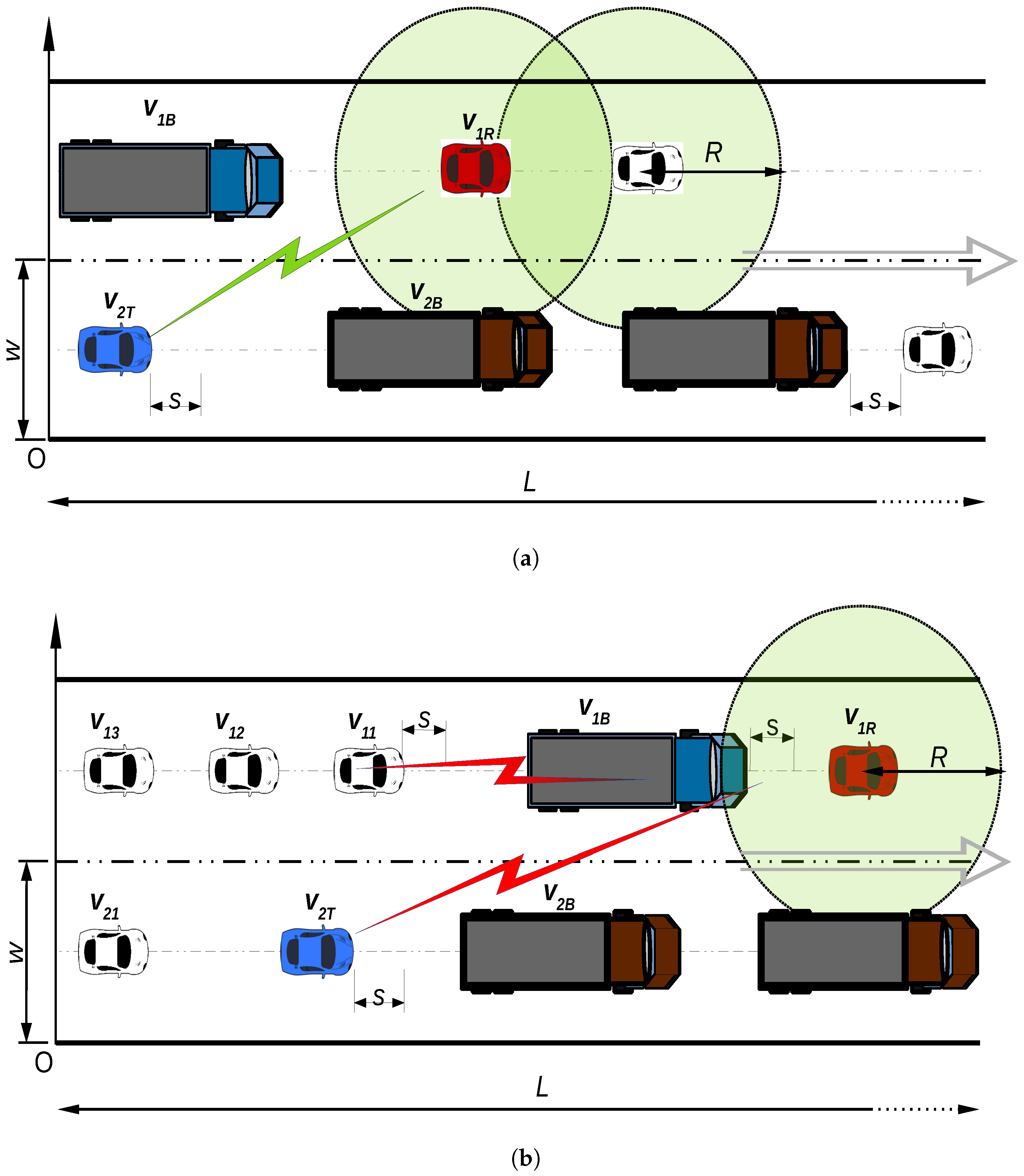
2. System Model
3. Analytical Procedure
3.1. Static Communication Ranges
3.2. Random Communications Ranges
3.2.1. Rayleigh Fading Channel Effect
3.2.2. Nakagami-m Fading Channel Effect
3.2.3. Weibull Fading Channel Effect
3.2.4. Lognormal Channel Shadowing Effect
3.3. Vehicle Velocity Distribution in Traffic
3.4. Single-Hop Inter-Vehicle Distance
3.4.1. Free-Flow Traffic
3.4.2. Synchronised Transition Traffic
3.4.3. Generalised Inter-Vehicle Distribution
3.5. Connection Probability Using Dynamic Communication Ranges
3.5.1. Case 1: Static Communication Range
3.5.2. Case 2: Random Distributed Communication Range
4. Discussion
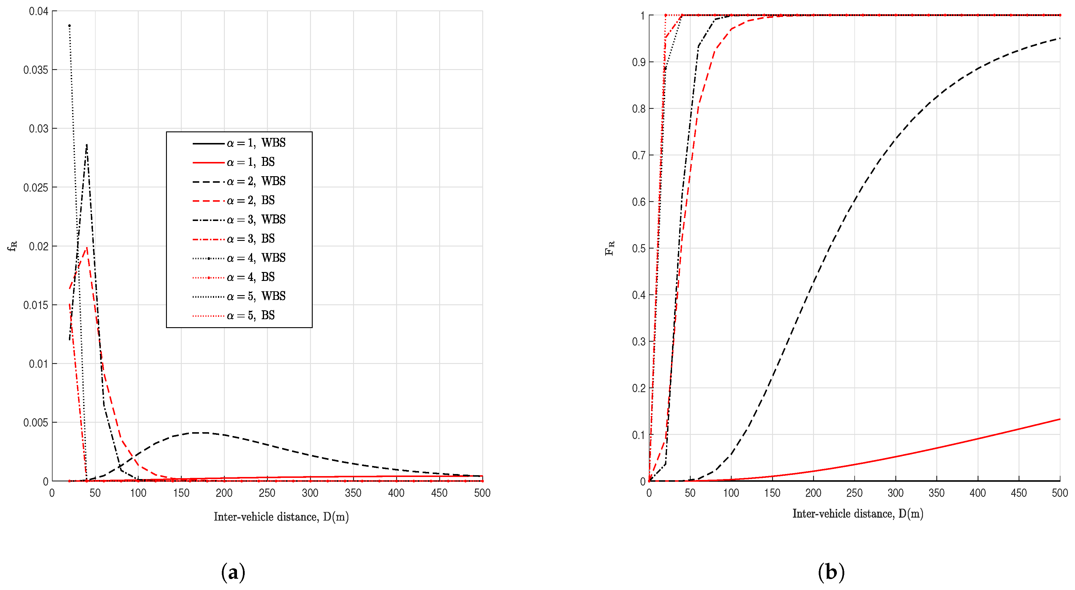
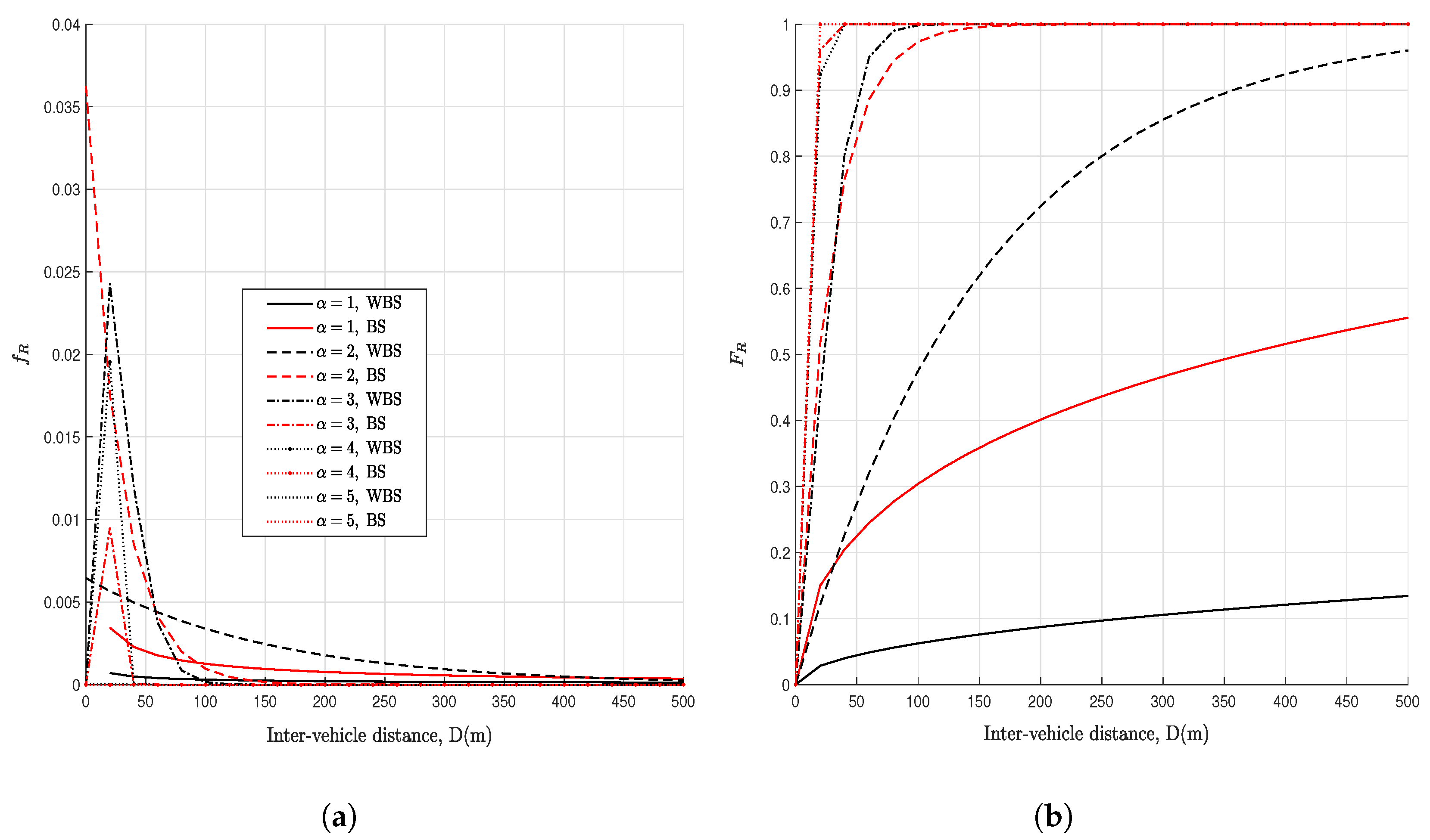
4.1. Distribution of Ranges
4.1.1. Lognormal Distributed Ranges
4.1.2. Rayleigh Distributed Ranges
4.1.3. Nakagami-m Distributed Ranges
4.1.4. Weibull Distributed Ranges
4.2. Single-Hop Probability of Connectivity
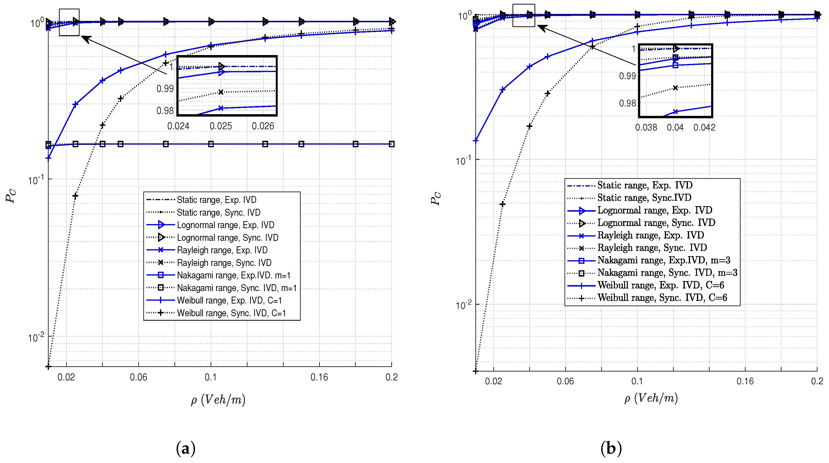
4.2.1. Connectivity with Density
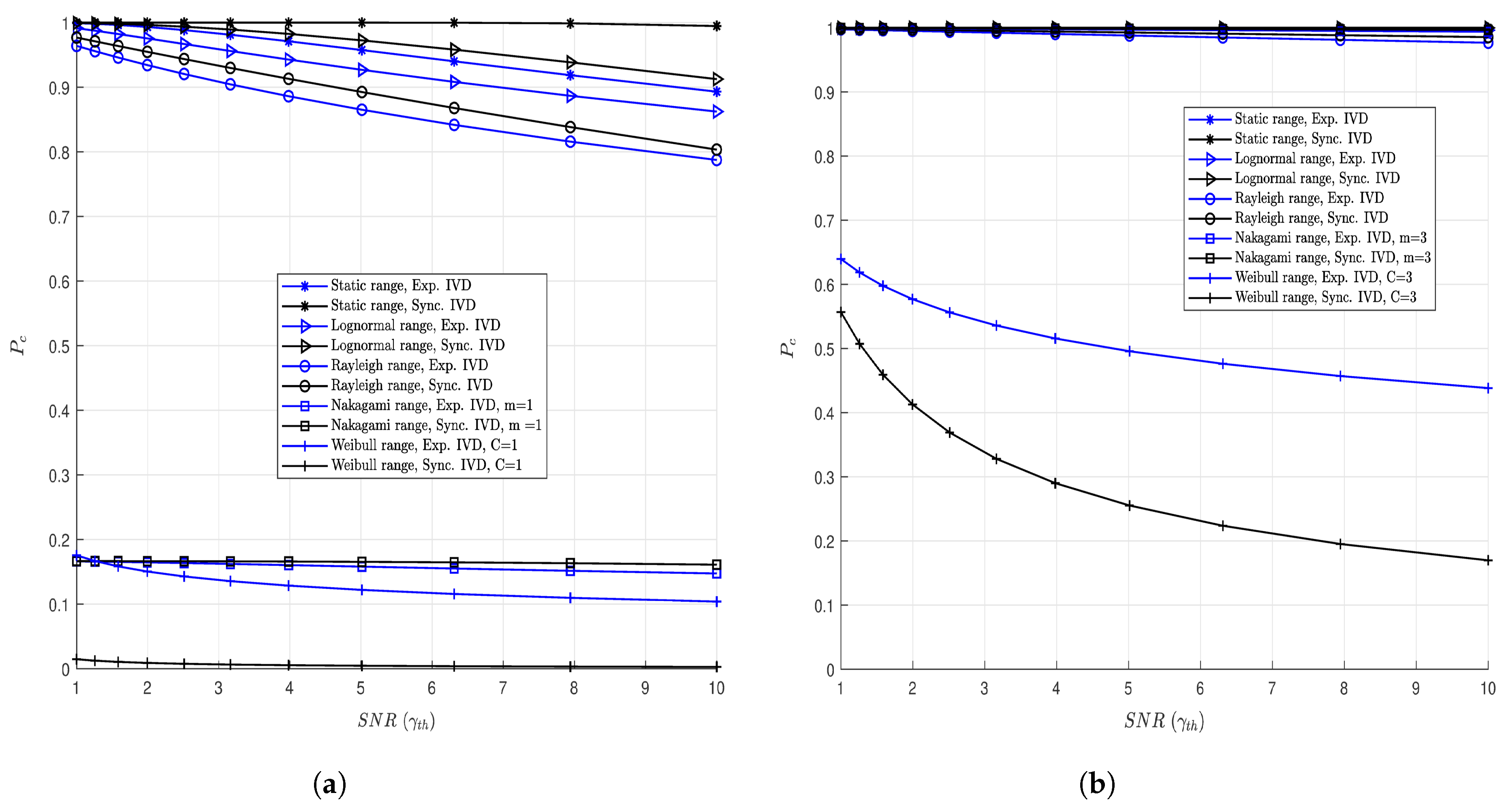
4.2.2. Connectivity with SNR
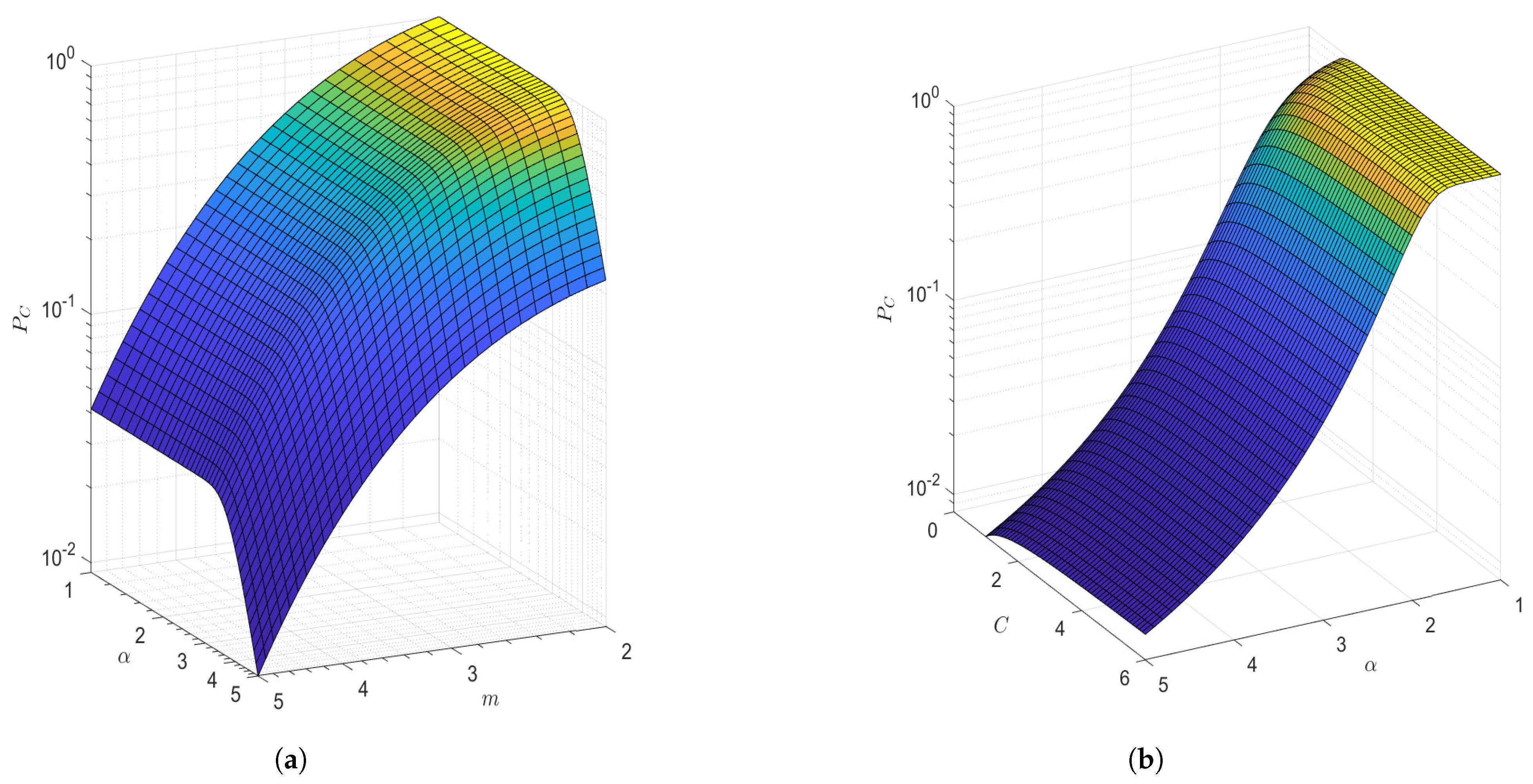
4.2.3. Connectivity with Path-Loss
4.3. Big Vehicle Shadowing Effect
4.3.1. Connectivity with Big Vehicle Prob
4.3.2. Connectivity with Number of Vehicles
4.4. General Observations
4.4.1. Synchronized Mobility
4.4.2. Exponential Mobility
5. Conclusions
Author Contributions
Funding
Data Availability Statement
Conflicts of Interest
Appendix A
Appendix B
References
- Al-Absi, M.A.; Abdulhakim, A.-A.A.; Lee, H.J. Performance Analysis for City, Highway, and Rural Area in Vehicle-to-Vehicle Network. In Proceedings of the 2018 International Conference on Information and Communication Technology Convergence (ICTC), Jeju, Republic of Korea, 17–19 October 2018; pp. 639–644. [Google Scholar]
- Dessai, S.F.; Sutar, D. Radio propagation model with obstacle effect and efficient bandwidth utilization for V2V VANET application services. In Proceedings of the 2019 International Conference on Intelligent Computing and Control Systems (ICCS), Madurai, India, 15–17 May 2019; pp. 602–606. [Google Scholar]
- Cui, Q.; Wang, N.; Haenggi, M. Vehicle Distributions in Large and Small Cities: Spatial Models and Applications. IEEE Trans. Veh. Technol. 2018, 67, 10176–10189. [Google Scholar] [CrossRef]
- Li, F.; Chen, W.; Shui, Y. Study on Connectivity Probability of Vanets Under Adverse Weather Conditions at 5.9 GHz. IEEE Access 2020, 8, 547–555. [Google Scholar] [CrossRef]
- Li, F.; Chen, W.; Wang, J.; Shui, Y.; Yang, K.; Xu, L.; Yu, J.; Li, C. Different Traffic Density Connectivity Probability Analysis in VANETs with Measured Data at 5.9 GHz. In Proceedings of the 16th International Conference on Intelligent Transportation Systems Telecommunications (ITST), Lisboa, Portugal, 15–17 October 2018; pp. 1–7. [Google Scholar]
- Li, X.; Zhou, R.; Zhou, T.; Liu, L.; Yu, K. Connectivity Probability Analysis for Green Cooperative Cognitive Vehicular Networks. IEEE Trans. Green Commun. Netw. 2022, 6, 1553–1563. [Google Scholar] [CrossRef]
- Jameel, F.; Haider, M.A.A.; Butt, A.A. Performance analysis of VANETs under Rayleigh, Rician, Nakagami-m and Weibull fading. In Proceedings of the International Conference on Communication, Computing and Digital Systems (C-CODE), Islamabad, Pakistan, 8–9 March 2017; pp. 127–132. [Google Scholar]
- Zeng, F.; Li, C.; Wang, H. Performance Evaluation of Different Fading Channels in Vehicular Ad Hoc Networks. In Proceedings of the International Conference on Information and Communication Technology Convergence (ICTC), Jeju, Republic of Korea, 17–19 October 2018; pp. 356–361. [Google Scholar]
- Wang, Y.; Xing, X.; Fan, J. Statistical Properties Evaluation on Rayleigh VANET Fading Channels. In Proceedings of the 6th International Conference on Wireless Communications Networking and Mobile Computing (WiCOM), Chengdu, China, 23–25 September 2010; pp. 1–6. [Google Scholar]
- Hu, M.; Zhong, Z.; Wu, H.; Ni, M. Effect of fading channel on link duration in Vehicular Ad Hoc Networks. In Proceedings of the 2013 IEEE Wireless Communications and Networking Conference (WCNC), Shanghai, China, 7–10 April 2013; pp. 1669–1673. [Google Scholar]
- Elaraby, S.; Abuelenin, S.M. Fading Improves Connectivity in Vehicular Ad-hoc Networks. arXiv 2019, arXiv:1910.05317. [Google Scholar]
- Rawat, D.B.; Shetty, S. Enhancing connectivity for spectrum-agile Vehicular Ad hoc NETworks in fading channels. In Proceedings of the 2014 IEEE Intelligent Vehicles Symposium, Dearborn, MI, USA, 8–11 June 2014; pp. 957–962. [Google Scholar]
- Nguyen, H.; Xu, X.; Noor-A-Rahim, M.; Guan, Y.L.; Pesch, D.; Li, H.; Filippi, A. Impact of Big Vehicle Shadowing on Vehicle-to-Vehicle Communications. IEEE Trans. Veh. Technol. 2020, 69, 6902–6915. [Google Scholar] [CrossRef]
- Alwane, S.K.; Siddle, D.R.; Stocker, A.J. The effect of the vehicle size on the V2V radio channel. In Proceedings of the Antennas and Propagation Conference (APC-2019), Birmingham, UK, 11–12 November 2019; pp. 1–4. [Google Scholar]
- Zhao, Y.; Xu, X.; Gao, Y. Selective Relaying Strategy for Vehicular Communication with Big-Vehicle Shadowing. In Proceedings of the 2021 IEEE 94th Vehicular Technology Conference (VTC2021-Fall), Norman, OK, USA, 27–30 September 2021; pp. 1–5. [Google Scholar]
- Chen, R.; Zhong, Z.; Leung, V.C.M.; Michelson, D.G. Performance Analysis of Connectivity for Vehicular Ad Hoc Networks with Moving Obstructions. In Proceedings of the 2014 IEEE 80th Vehicular Technology Conference (VTC2014-Fall), Vancouver, BC, Canada, 14–17 September 2014; pp. 1–5. [Google Scholar]
- Vlastaras, D.; Whiton, R.; Tufvesson, F. A model for power contributions from diffraction around a truck in vehicle-to-vehicle communications. In Proceedings of the 15th International Conference on ITS Telecommunications (ITST), Warsaw, Poland, 29–31 May 2017; pp. 1–6. [Google Scholar]
- Yang, M.; Ai, B.; He, R.; Chen, L.; Li, X.; Huang, Z.; Li, J.; Huang, C. Path Loss Analysis and Modeling for Vehicle-to-Vehicle Communications with Vehicle Obstructions. In Proceedings of the 10th International Conference on Wireless Communications and Signal Processing (WCSP), Hangzhou, China, 18–20 October 2018; pp. 1–6. [Google Scholar]
- Abuelenin, S.M.; Elaraby, S.A. Generalized Framework for Connectivity Analysis in Vehicle-to-Vehicle Communications. IEEE Trans. Intell. Transp. Syst. 2022, 23, 5894–5898. [Google Scholar] [CrossRef]
- Babu, A.V.; Muhammed Ajeer, V.K. Analytical model for connectivity of vehicular ad hoc networks in the presence of channel randomness. Int. J. Commun. Syst. 2011, 26, 927–946. [Google Scholar] [CrossRef]
- The MathWorks, Inc. Optimization Toolbox Version: 9.4 (R2023a). 2023. Available online: https://www.mathworks.com (accessed on 1 January 2023).
- Goldsmith, A. Wireless Communications; Cambridge University Press: Cambridge, UK, 2005. [Google Scholar]
- Nagel, R. The effect of vehicular distance distributions and mobility on VANET communications. In Proceedings of the 2010 IEEE Intelligent Vehicles Symposium, La Jolla, CA, USA, 21–24 June 2010; pp. 1190–1194. [Google Scholar]
- Cheng, J.; Tellambura, C.; Beaulieu, N.C. Performance of digital linear modulations on Weibull slow-fading channels. IEEE Trans. Commun. 2004, 52, 1265–1268. [Google Scholar] [CrossRef]
- Zhao, J.; Chen, Y.; Gong, Y. Study of Connectivity Probability of Vehicle-to-Vehicle and Vehicle-to-Infrastructure Communication Systems. In Proceedings of the IEEE 83rd Vehicular Technology Conference (VTC Spring), Nanjing, China, 15–18 May 2016; pp. 1–4. [Google Scholar]
- Ross, S. Introduction to Probability Models, 11th ed.; Academic Press: Cambridge, MA, USA, 2014. [Google Scholar]
- Gradshteyn, I.S.; Ryzhik, I.M.; Jeffrey, A.; Zwillinger, D. Table of Integrals, Series, And Products, 7th ed.; Elsevier: London, UK, 2007. [Google Scholar]
- Yousefi, S.; Altman, E.; El-Azouzi, R.; Fathy, M. Analytical Model for Connectivity in Vehicular Ad Hoc Networks. IEEE Trans. Veh. Technol. 2008, 57, 3341–3356. [Google Scholar] [CrossRef]
- Zhang, Z.; Mao, G.; Anderson, B.D.O. On the Information Propagation Process in Mobile Vehicular Ad Hoc Networks. IEEE Trans. Veh. Technol. 2011, 60, 2314–2325. [Google Scholar] [CrossRef]
- Chen, C.; Liu, L.; Du, X.; Wei, X.; Pei, C. Available connectivity analysis under free flow state in VANETs. J. Wirel. Commun. Netw. 2012, 2012, 270. [Google Scholar] [CrossRef]
- Li, C.; Zhen, A.; Sun, J.; Zhang, M.; Hu, X. Analysis of connectivity probability in VANETs considering minimum safety distance. In Proceedings of the 8th International Conference on Wireless Communications and Signal Processing (WCSP), Yangzhou, China, 13–15 October 2016; pp. 1–5. [Google Scholar]
- Beals, R.; Szmisgielski, J. Meijer G-functions: A Gentle Introduction. Not. Am. Math. Soc. 2013, 60, 866–872. [Google Scholar] [CrossRef]


| Notation | Value |
|---|---|
| Transmitted power | |
| Noise power | |
| Signal-to-noise ratio (SNR) threshold | |
| G-Meijer function [21] | |
| Error function | |
| Traffic headway distribution mapping factor | |
| Vehicle density | |
| m | Nakagami-m fading factor |
| C | Weibull factor |
| Pathloss exponent | |
| Weibull fading pathloss exponent | |
| Big vehicle availability probability | |
| C | Weibull factor |
| Big vehicle pathloss |
| Channel Model | |||
|---|---|---|---|
| Pathloss | – | – | |
| Rayleigh fading | |||
| Nakagami-m fading | |||
| Weibull fading | |||
| Lognormal shadowing |
| Connectivity Probability | Free-Flow Traffic | Synchronised Traffic |
|---|---|---|
| Static range | ||
| Rayleigh range | ||
| Nakagami-m range | ||
| Weibull range | ||
| Lognormal range |
| Parameter | Notation | Value |
|---|---|---|
| Mean speed | [70, 90, 110, 130, 150] (km/h) | |
| Speed std | [21, 27, 33, 39, 45] (km/h) | |
| Road length | L | 4 km |
| Inter-vehicle distance | D | [10–1000] (m) |
| Lane width | W | 3 m |
| Arrival rate | 0.1 veh/s | |
| Transmit power | 0.5 W | |
| Noise power | mW | |
| Pathloss constant | K | 10 |
| Pathloss exponent | [1–5] | |
| Threshold SNR | 10.17 dB |
Disclaimer/Publisher’s Note: The statements, opinions and data contained in all publications are solely those of the individual author(s) and contributor(s) and not of MDPI and/or the editor(s). MDPI and/or the editor(s) disclaim responsibility for any injury to people or property resulting from any ideas, methods, instructions or products referred to in the content. |
© 2025 by the authors. Licensee MDPI, Basel, Switzerland. This article is an open access article distributed under the terms and conditions of the Creative Commons Attribution (CC BY) license (https://creativecommons.org/licenses/by/4.0/).
Share and Cite
Okello, K.; Mwangi, E.; El-Malek, A.H.A. Connectivity Analysis in VANETS with Dynamic Ranges. Telecom 2025, 6, 33. https://doi.org/10.3390/telecom6020033
Okello K, Mwangi E, El-Malek AHA. Connectivity Analysis in VANETS with Dynamic Ranges. Telecom. 2025; 6(2):33. https://doi.org/10.3390/telecom6020033
Chicago/Turabian StyleOkello, Kenneth, Elijah Mwangi, and Ahmed H. Abd El-Malek. 2025. "Connectivity Analysis in VANETS with Dynamic Ranges" Telecom 6, no. 2: 33. https://doi.org/10.3390/telecom6020033
APA StyleOkello, K., Mwangi, E., & El-Malek, A. H. A. (2025). Connectivity Analysis in VANETS with Dynamic Ranges. Telecom, 6(2), 33. https://doi.org/10.3390/telecom6020033