Clustering for Lifetime Enhancement in Wireless Sensor Networks


Abstract
1. Introduction
2. Related Work
3. Advanced Clustering Approach
3.1. Parameters That Affect Clustering Efficiency
3.2. Parameters Considered in the LEACH Energy Model
3.3. Clustering Efficiency: Analysis Study
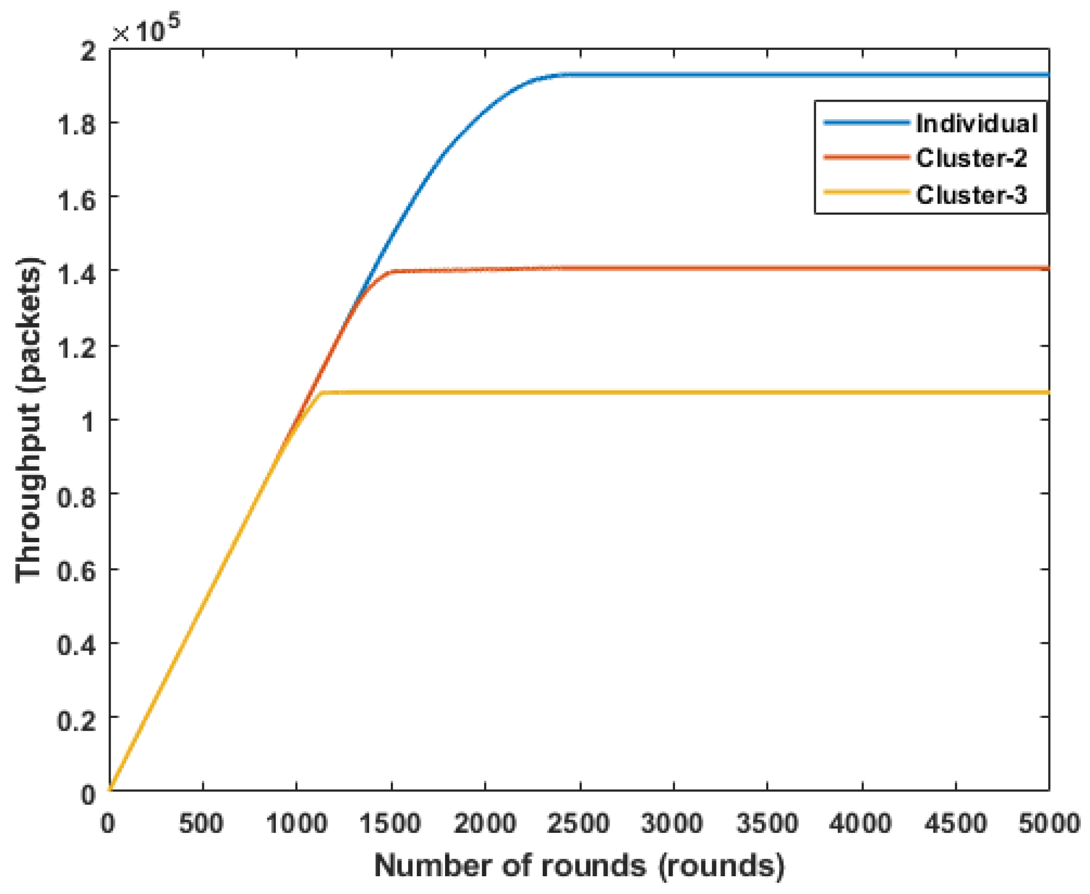
4. Simulation Results
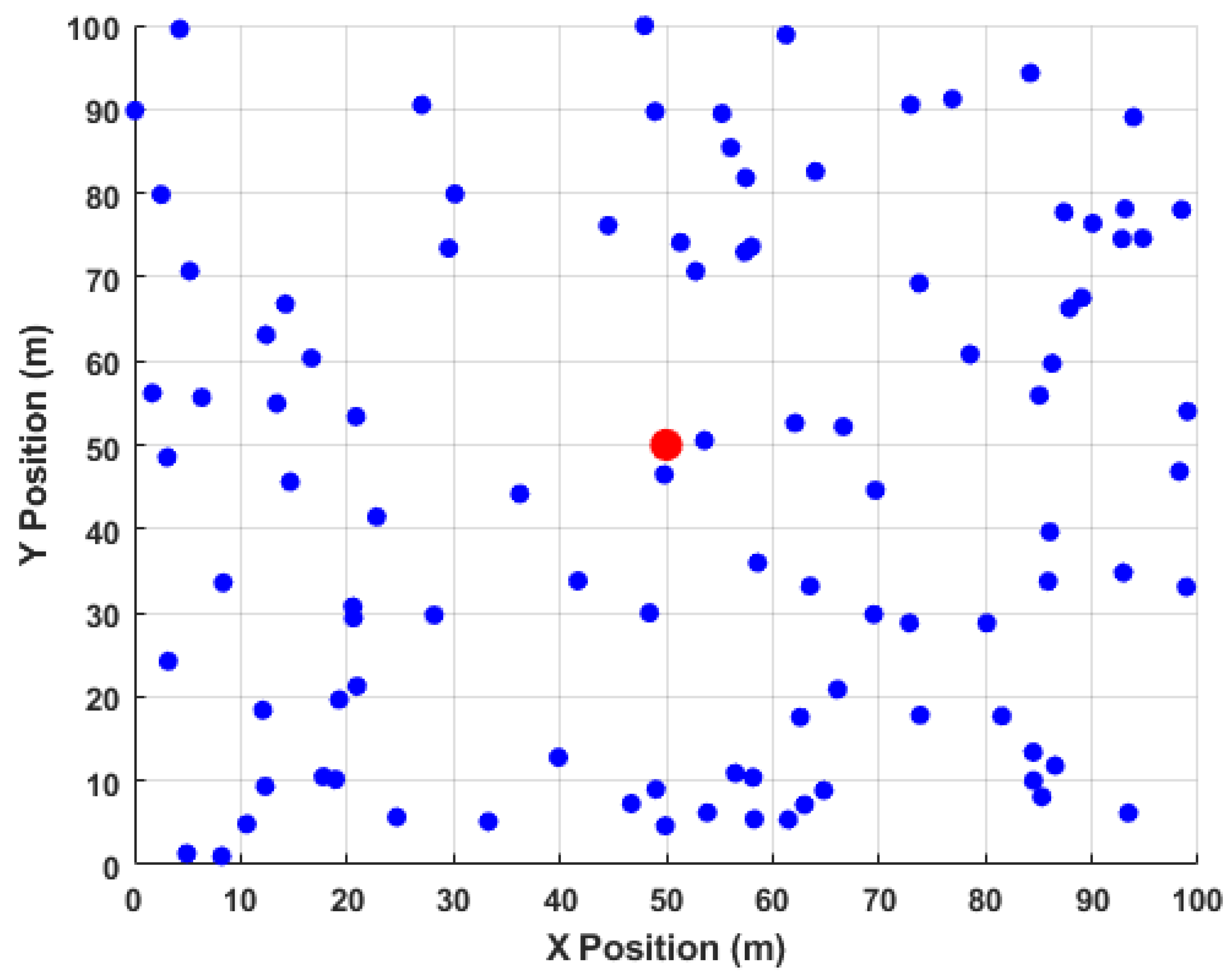
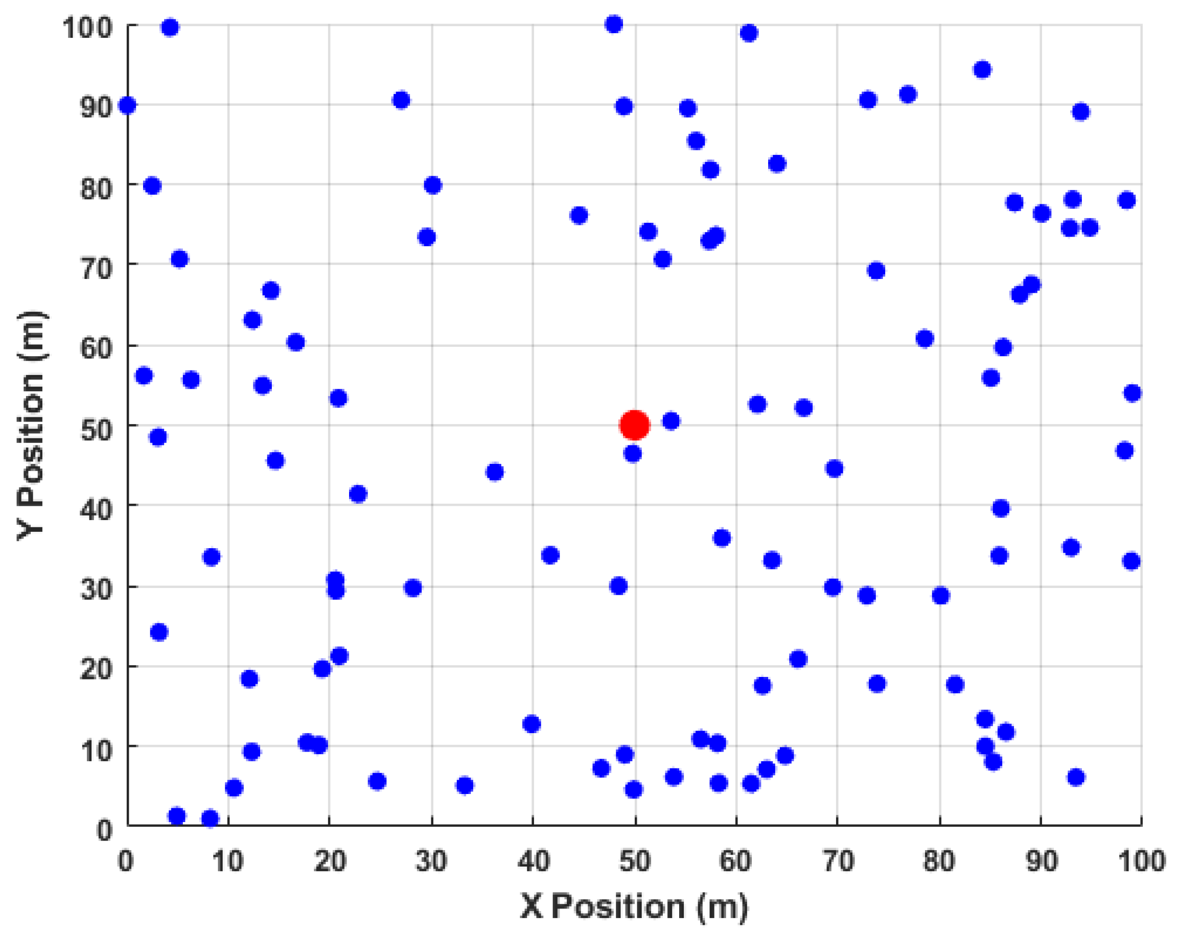
4.1. First Scenario: The Base Station (BS) Is Located at the Center of the Area (50, 50)
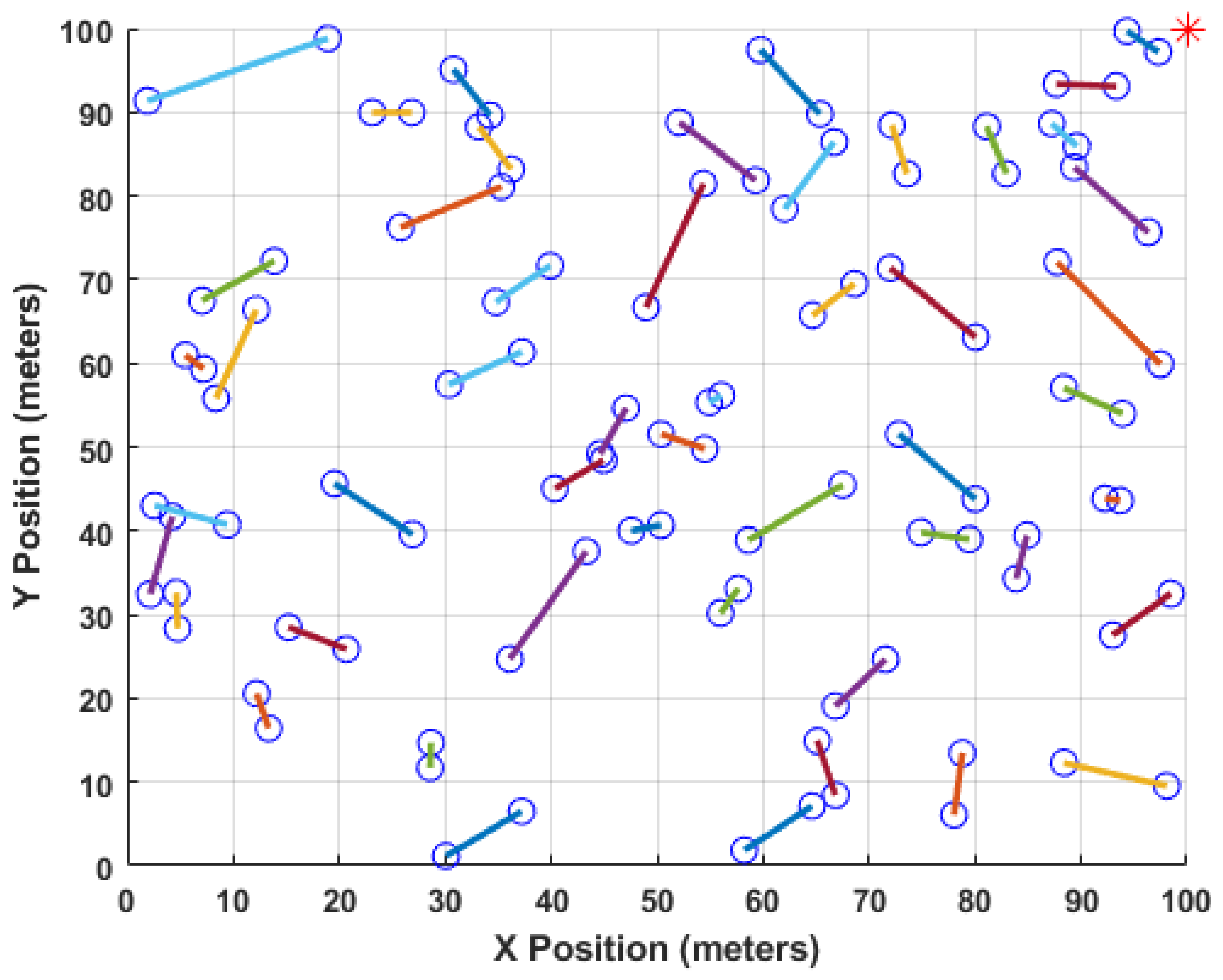
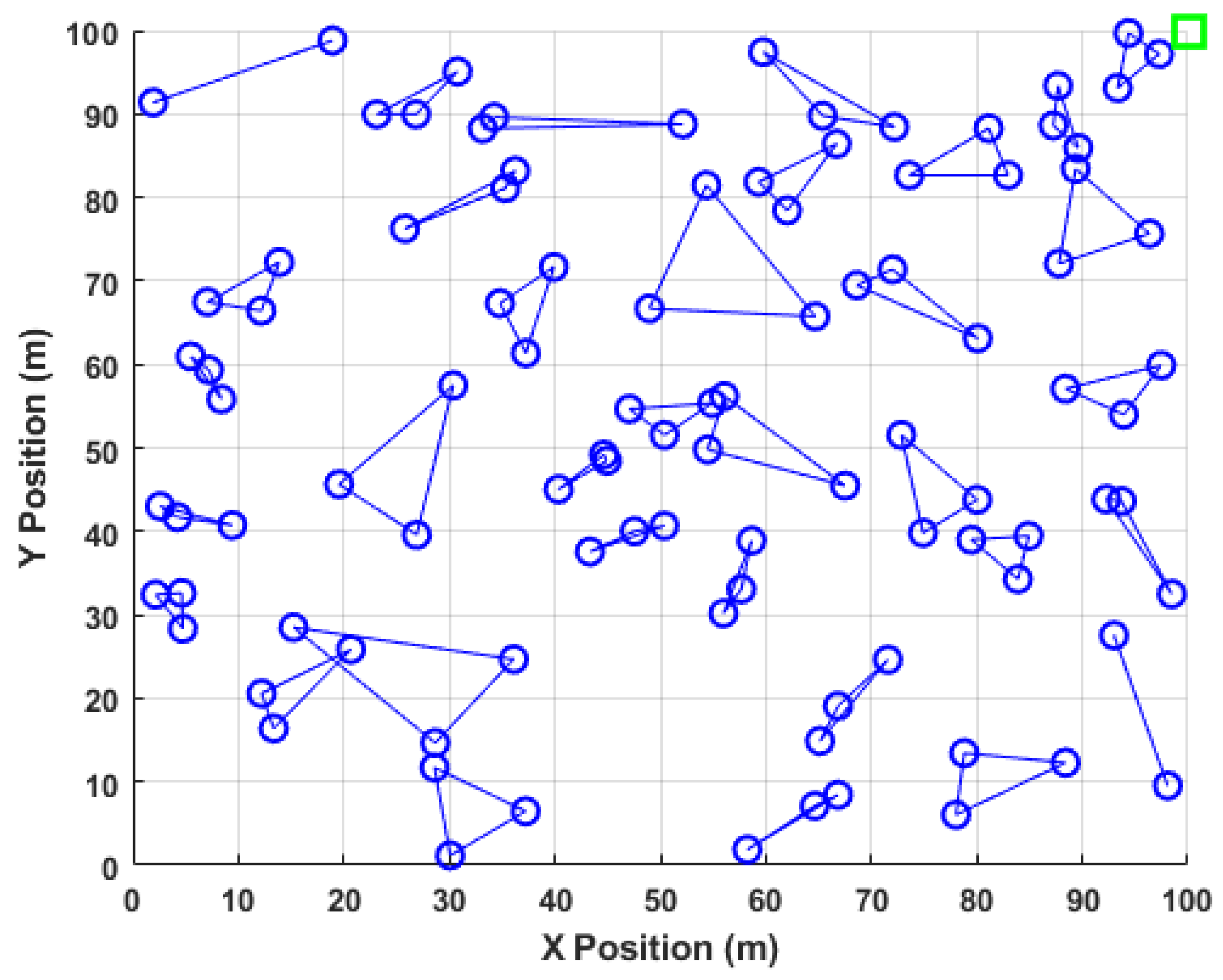
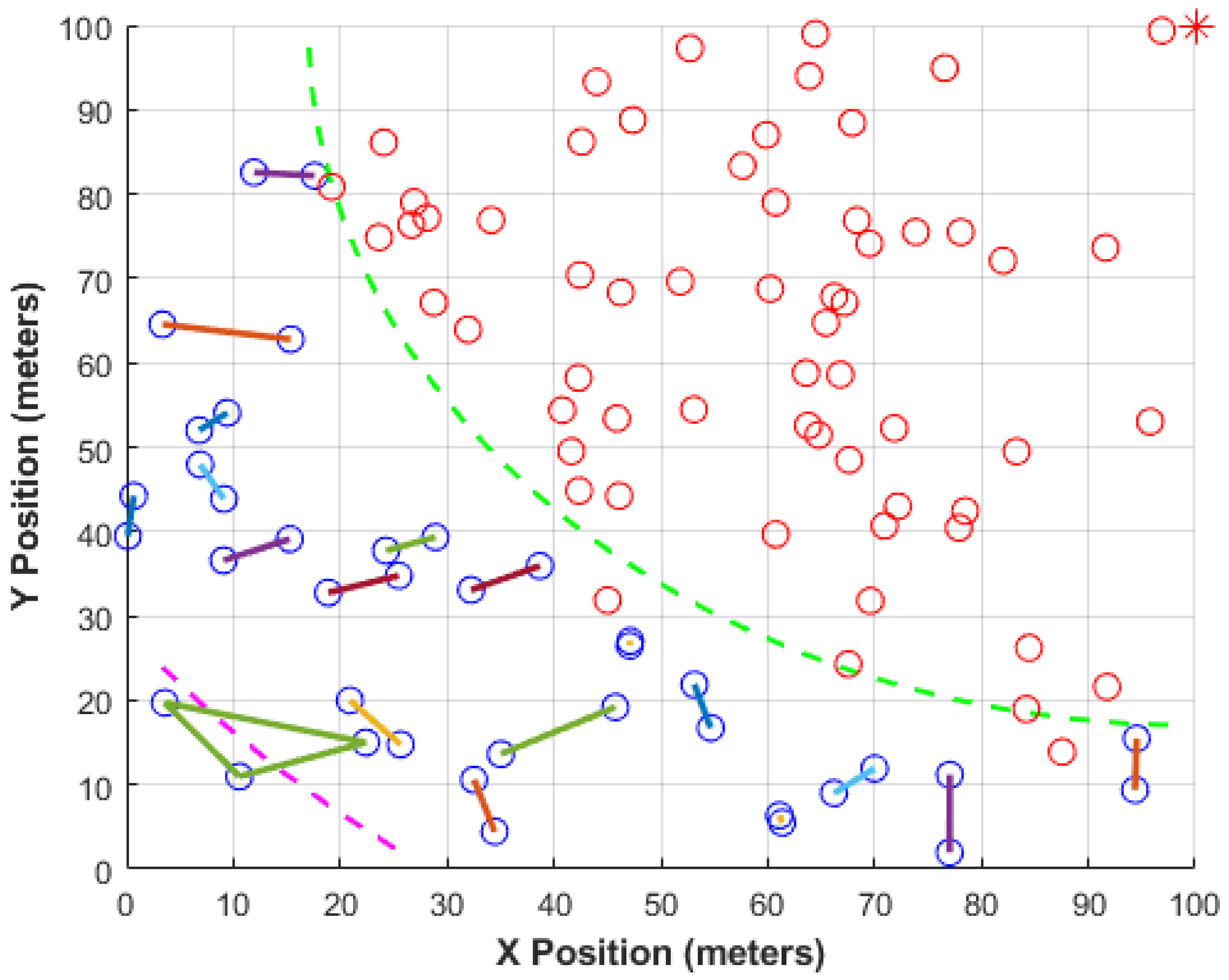
4.2. Second Scenario: The Base Station (BS) Is Located at the Center of the Area (100, 100)
5. Conclusions
Author Contributions
Funding
Data Availability Statement
Conflicts of Interest
References
- Sahoo, L.; Sen, S.; Tiwary, K.S.; Moslem, S.; Senapati, T. Improvement of Wireless Sensor Network Lifetime via Intelligent Clustering Under Uncertainty. IEEE Access 2024, 12, 25018–25033. [Google Scholar] [CrossRef]
- Al-Sulaifanie, A.I.; Al-Sulaifanie, B.K.; Biswas, S. Recent trends in clustering algorithms for wireless sensor networks: A comprehensive review. Comput. Commun. 2022, 191, 395–424. [Google Scholar] [CrossRef]
- Kanchi, S. Clustering Algorithm For Wireless Sensor Networks With Balanced Cluster Size. Procedia Comput. Sci. 2024, 238, 119–126. [Google Scholar] [CrossRef]
- Abose, T.A.; Tekulapally, V.; Megersa, K.T.; Kejela, D.C.; Daka, S.T.; Jember, K.A. Improving wireless sensor network lifespan with optimized clustering probabilities, improved residual energy LEACH and energy efficient LEACH for corner-positioned base stations. Heliyon 2024, 10, e34382. [Google Scholar] [CrossRef]
- Merabtine, N.; Djenouri, D.; Zegour, D.E. Towards energy efficient clustering in wireless sensor networks: A comprehensive review. IEEE Access 2021, 9, 92688–92705. [Google Scholar] [CrossRef]
- Nedham, W.B.; Al-Qurabat, A.K.M. A comprehensive review of clustering approaches for energy efficiency in wireless sensor networks. Int. J. Comput. Appl. Technol. 2023, 72, 139–160. [Google Scholar] [CrossRef]
- Hussain, M.H.A.; Mokhtar, B.; Rizk, M.R. A comparative survey on LEACH successors clustering algorithms for energy-efficient longevity WSNs. Egypt. Inform. J. 2024, 26, 100477. [Google Scholar] [CrossRef]
- Adumbabu, I.; Selvakumar, K. An Improved Lifetime and Energy Consumption with Enhanced Clustering in WSNs. Intell. Autom. Soft Comput. 2023, 35, 1939–1956. [Google Scholar] [CrossRef]
- Kumar, N.; Rani, P.; Kumar, V.; Verma, P.K.; Koundal, D. TEEECH: Three-tier extended energy efficient clustering hierarchy protocol for heterogeneous wireless sensor network. Expert Syst. Appl. 2023, 216, 119448. [Google Scholar] [CrossRef]
- Gupta, A.D.; Rout, R.K. SMEOR: Sink mobility-based energy-optimized routing in energy harvesting-enabled wireless sensor network. Int. J. Commun. Syst. 2023, 37, e5679. [Google Scholar] [CrossRef]
- Heinzelman, W.R.; Chandrakasan, A.; Balakrishnan, H. Energy-efficient communication protocol for wireless microsensor networks. In Proceedings of the 33rd Annual Hawaii International Conference on System Sciences, Maui, HI, USA, 7 January 2000; IEEE: Piscataway, NJ, USA, 2000; pp. 1–10. [Google Scholar]
- Daanoune, I.; Baghdad, A.; Ballouk, A. Improved LEACH protocol for increasing the lifetime of WSNs. Int. J. Electr. Comput. Eng. 2021, 11, 3106–3113. [Google Scholar] [CrossRef]
- Dwivedi, A.K.; Sharma, A.K. EE-LEACH: Energy enhancement in LEACH using fuzzy logic for homogeneous WSN. Wirel. Pers. Commun. 2021, 120, 3035–3055. [Google Scholar] [CrossRef]
- Pour, S.E.; Javidan, R. A new energy aware cluster head selection for LEACH in wireless sensor networks. IET Wirel. Sens. Syst. 2021, 11, 45–53. [Google Scholar] [CrossRef]
- Abdulaal, A.H.; Shah, A.F.M.S.; Pathan, A.K. NM-LEACH: A novel modified LEACH protocol to improve performance in WSN. Int. J. Commun. Netw. Inf. Secur. 2022, 14, 1–10. [Google Scholar] [CrossRef]
- Suleiman, H.; Hamdan, M. Adaptive probabilistic model for energy-efficient distance-based clustering in WSNs (Adapt-P): A LEACH-based analytical study. arXiv 2021, arXiv:2110.13300. [Google Scholar]
- Sennan, S.; Alotaibi, Y.; Pandey, D.; Alghamdi, S. EACR-LEACH: Energy-Aware Cluster-based Routing Protocol for WSN Based IoT. Comput. Mater. Contin. 2022, 72, 2159–2173. [Google Scholar] [CrossRef]
- Shafiq, M.; Ashraf, H.; Ullah, A.; Masud, M.; Azeem, M.; Jhanjhi, N.Z.; Humayun, M. Robust cluster-based routing protocol for IoT-assisted smart devices in WSN. Comput. Mater. Contin. 2021, 67, 3505–3521. [Google Scholar] [CrossRef]
- Suresh, K.; Mole, S.S.S.; Kumar, A.J.S. F2SO: An energy efficient cluster based routing protocol using fuzzy firebug swarm optimization algorithm in WSN. Comput. J. 2023, 66, 1126–1138. [Google Scholar] [CrossRef]
- Djabour, D.; Abidi, W.; Ezzedine, T. Fuzzy independent circular zones protocol for heterogeneous wireless sensor networks. Int. J. Ad Hoc Ubiquitous Comput. 2022, 39, 157–169. [Google Scholar] [CrossRef]
- Wang, H.; Liu, K.; Wang, C.; Hu, H. Energy-Efficient, Cluster-Based Routing Protocol for Wireless Sensor Networks Using Fuzzy Logic and Quantum Annealing Algorithm. Sensors 2024, 24, 4105. [Google Scholar] [CrossRef]
- Alghamdi, T.A. Energy efficient protocol in wireless sensor network: Optimized cluster head selection model. Telecommun. Syst. 2020, 74, 331–345. [Google Scholar] [CrossRef]
- Narayan, V.; Daniel, A.K. RBCHS: Region-based cluster head selection protocol in wireless sensor network. In Proceedings of Integrated Intelligence Enable Networks and Computing: IIENC 2020; Springer: Singapore, 2021; pp. 863–869. [Google Scholar]


| Protocol | Cluster-Based | CH Selection Criteria | Routing Strategy | Key Contribution/Feature |
|---|---|---|---|---|
| LEACH [11] | Yes | Random selection | Single-hop to BS | Foundational protocol, random CH selection |
| Improved LEACH [12] | Yes | Residual energy, density | Single/multi-hop | Balanced CH workload withdensity awareness |
| EE-LEACH [13] | Yes | Residual energy, density, distance to BS (fuzzy logic) | Not specified | Avoids hotspot, fuzzy logic-based ranking |
| Energy-aware LEACH [14] | Yes | Residual energy, position centrality | Not specified | Adaptive CH range based on density |
| NM-LEACH [15] | Yes | Residual energy, distance to BS | Not specified | Even CH distribution, improved stability |
| Adaptive low energy [16] | Yes | Centrality, residual energy | Not specified | Minimizes intra-cluster distance |
| EACR-LEACH [17] | Yes | Residual energy, number of neighbors, CH load history | Not specified | Controls fairness in CH load |
| RCBRP [18] | Yes | Residual energy, distance, energy cost | Clustered routing | Optimized path for energy balance |
| Honey Badger-based [19] | Yes | Distance, residual energy, neighbors’ degree, centrality | Fuzzy swarm optimization | Hybrid metaheuristic CH selection |
| FICZP [20] | Yes | Lifetime of neighbors, residual energy, member lifetime | Fuzzy system | Energy-aware fuzzy zone-based clustering |
| Fuzzy-quantum annealing [21] | Yes | Residual energy, number of neighbors, distance, centrality | Quantum routing | Energy thresholding, hybrid IA |
| Dragonfly–firefly hybrid [22] | Yes | Energy, delay, distance, security | Hybrid metaheuristic | Focus on secure and efficient CHs |
| RBCHS [23] | Yes | Distance to BS, residual energy, number of neighbors | Static clusters + hybrid routing | Heterogeneous networks, zoned CH selection |
| Our approach | Yes | Distance to BS, a controlled density | Static topology, adaptive and zone-based, optimal strategy changes with distance from BS | Mathematically validated, proved that clustering is not always optimal; |
| Parameter | Value |
|---|---|
| Packet length (4000 bits). | |
| Energy dissipated to run the transmitter or receiver circuitry (50 nJ/bit). | |
| Transmitter amplifier, energy-free space model (10 pJ/bit/m2). | |
| Transmitter amplifier, energy multipath model (0.0013 pJ/bit/m4). | |
| Distance (m). | |
| Approximately . | |
| Number of packets. |
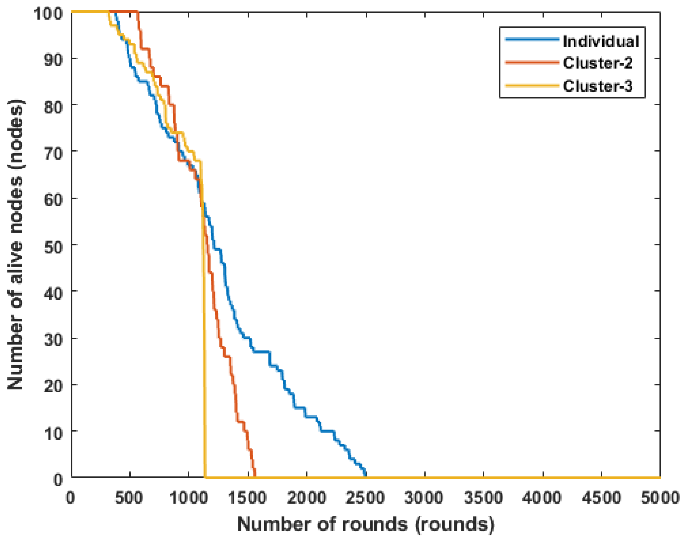
| Topology | FDN | MDN | LDN |
|---|---|---|---|
| Individual | 1340 | 1912 | 2496 |
| Cluster-2 | 1229 | 1361 | 1541 |
| Cluster-3 | 816 | 1118 | 1137 |
| Topology | FDN | MDN | LDN |
|---|---|---|---|
| Individual | 302 | 1056 | 2477 |
| Cluster-2 | 477 | 1084 | 2477 |
| Cluster-3 | 264 | 1121 | 2187 |
| Topology | FDN | MDN | LDN |
|---|---|---|---|
| Individual | 330 | 1142 | 2495 |
| Cluster-2 | 510 | 1113 | 2495 |
| Cluster-3 | 628 | 1140 | 2495 |
Disclaimer/Publisher’s Note: The statements, opinions and data contained in all publications are solely those of the individual author(s) and contributor(s) and not of MDPI and/or the editor(s). MDPI and/or the editor(s) disclaim responsibility for any injury to people or property resulting from any ideas, methods, instructions or products referred to in the content. |
© 2025 by the authors. Licensee MDPI, Basel, Switzerland. This article is an open access article distributed under the terms and conditions of the Creative Commons Attribution (CC BY) license (https://creativecommons.org/licenses/by/4.0/).
Share and Cite
Khedhiri, K.; Ben Omrane, I.; Djabour, D.; Cherif, A. Clustering for Lifetime Enhancement in Wireless Sensor Networks. Telecom 2025, 6, 30. https://doi.org/10.3390/telecom6020030
Khedhiri K, Ben Omrane I, Djabour D, Cherif A. Clustering for Lifetime Enhancement in Wireless Sensor Networks. Telecom. 2025; 6(2):30. https://doi.org/10.3390/telecom6020030
Chicago/Turabian StyleKhedhiri, Kamel, Ines Ben Omrane, Djamal Djabour, and Adnen Cherif. 2025. "Clustering for Lifetime Enhancement in Wireless Sensor Networks" Telecom 6, no. 2: 30. https://doi.org/10.3390/telecom6020030
APA StyleKhedhiri, K., Ben Omrane, I., Djabour, D., & Cherif, A. (2025). Clustering for Lifetime Enhancement in Wireless Sensor Networks. Telecom, 6(2), 30. https://doi.org/10.3390/telecom6020030