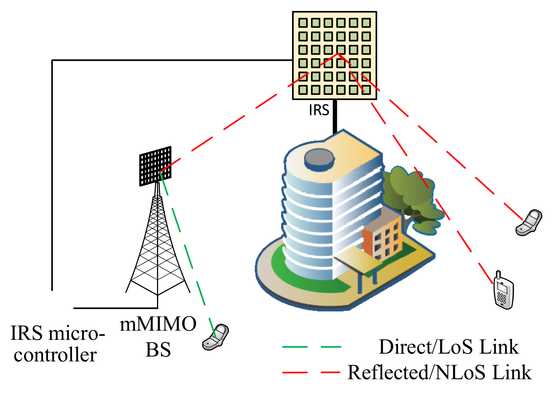
Figure 1.
Illustration of a Reconfigurable Intelligent Surface (RIS)-assisted communication system.
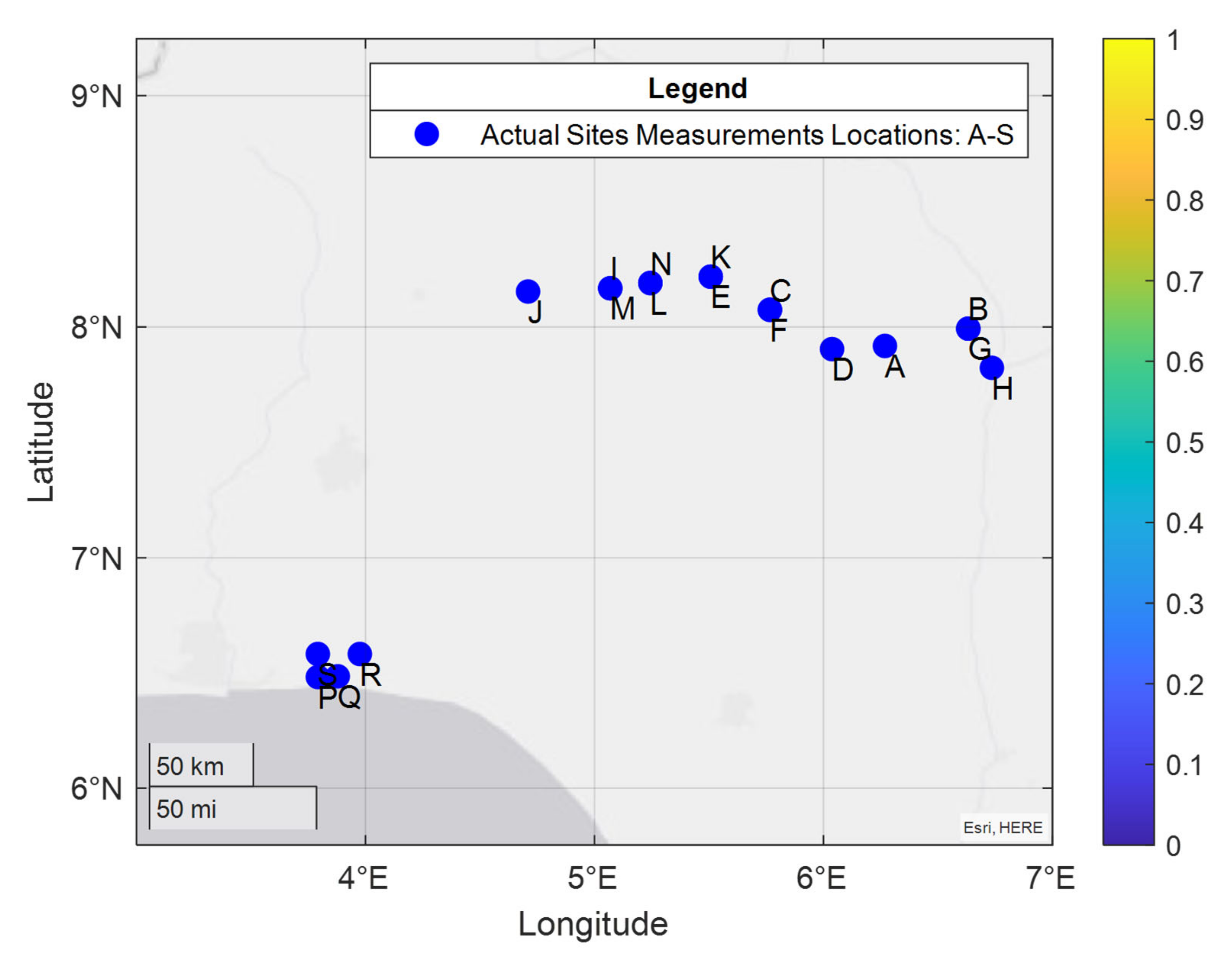
Figure 2.
The geographical coordinates of the measurement environments.
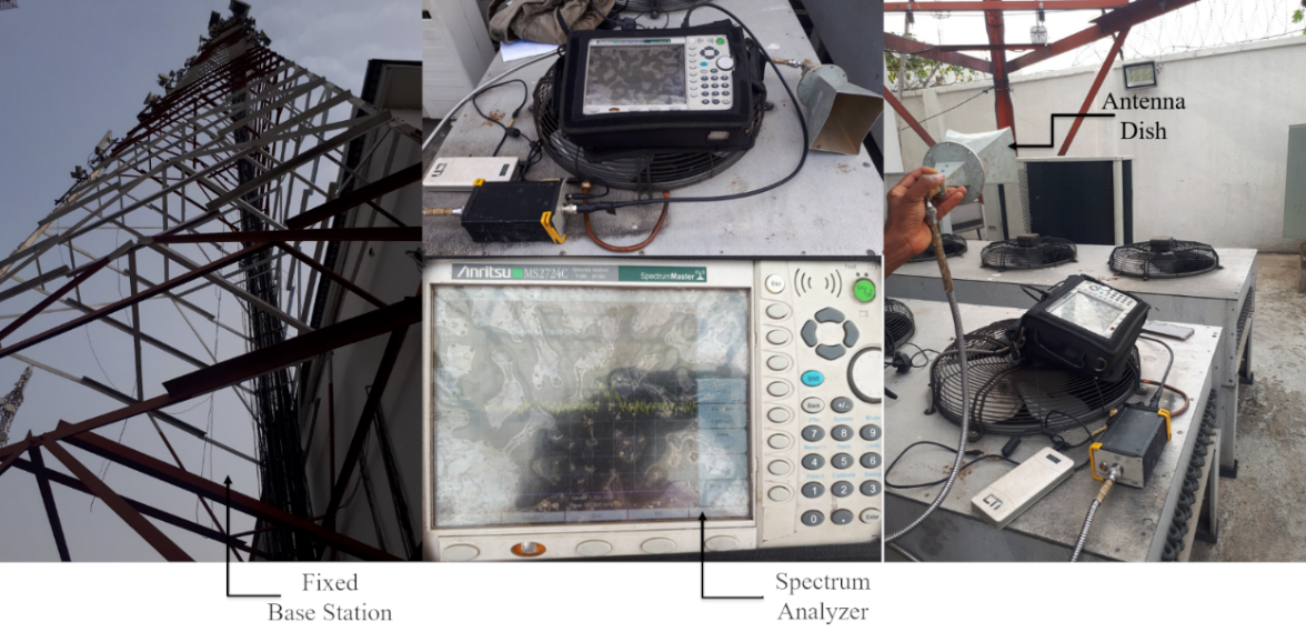
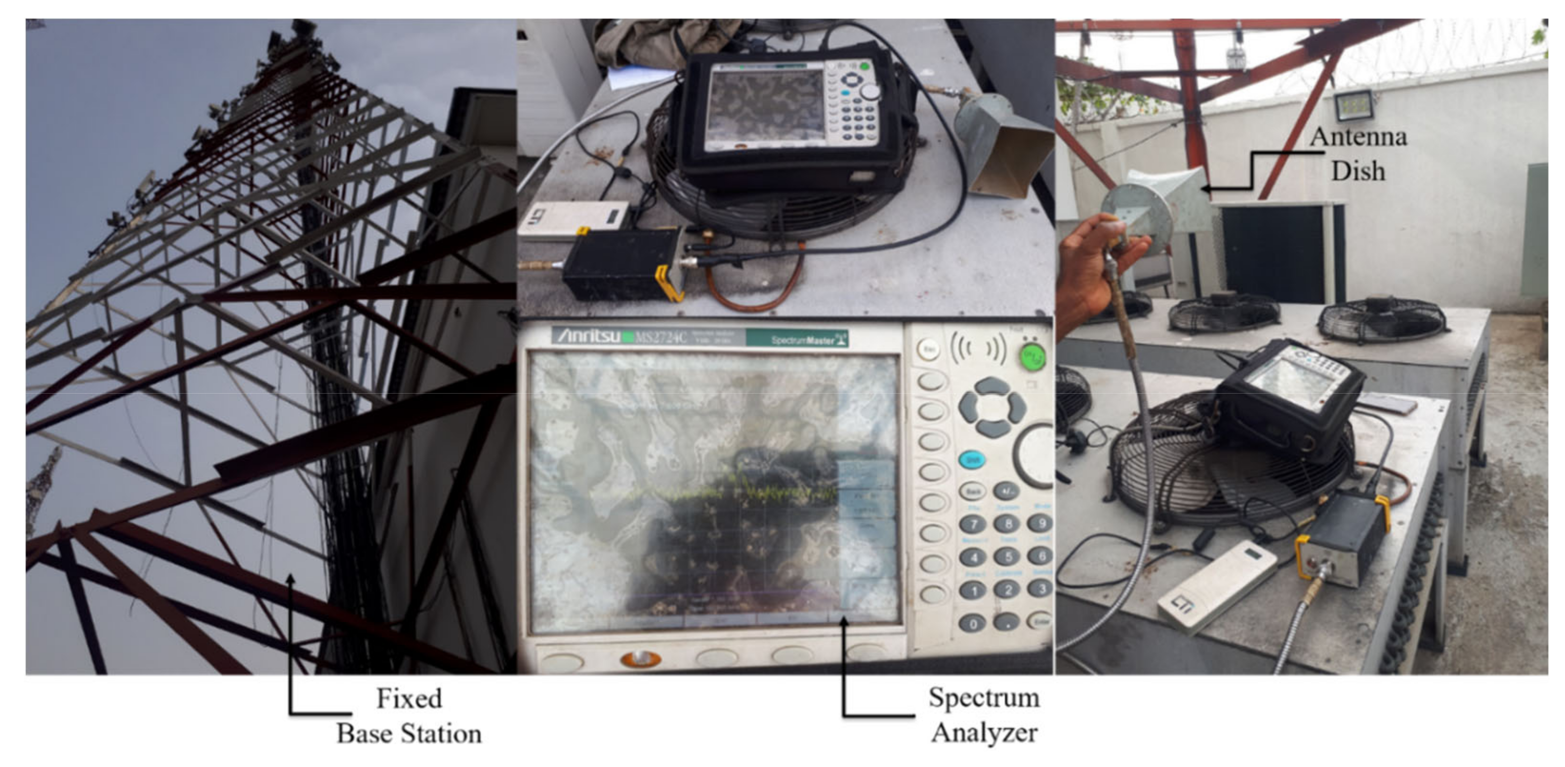
Figure 3.
Experimental setup for the frequency scan measurements.
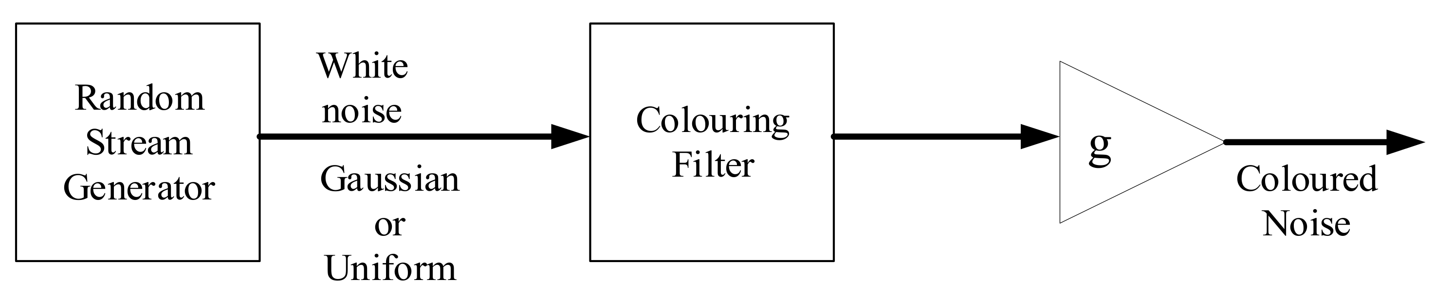
Figure 4.
Process of generating colored noise.
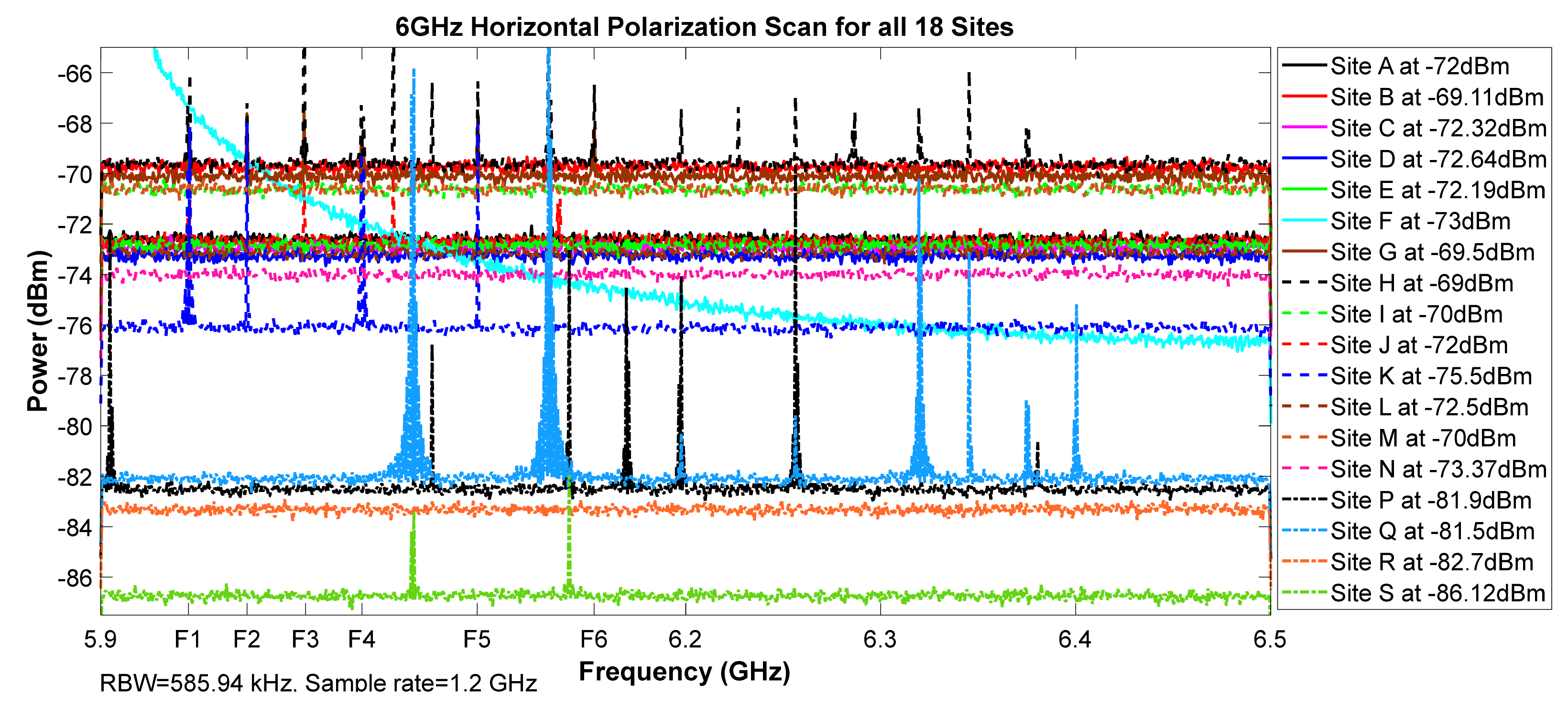
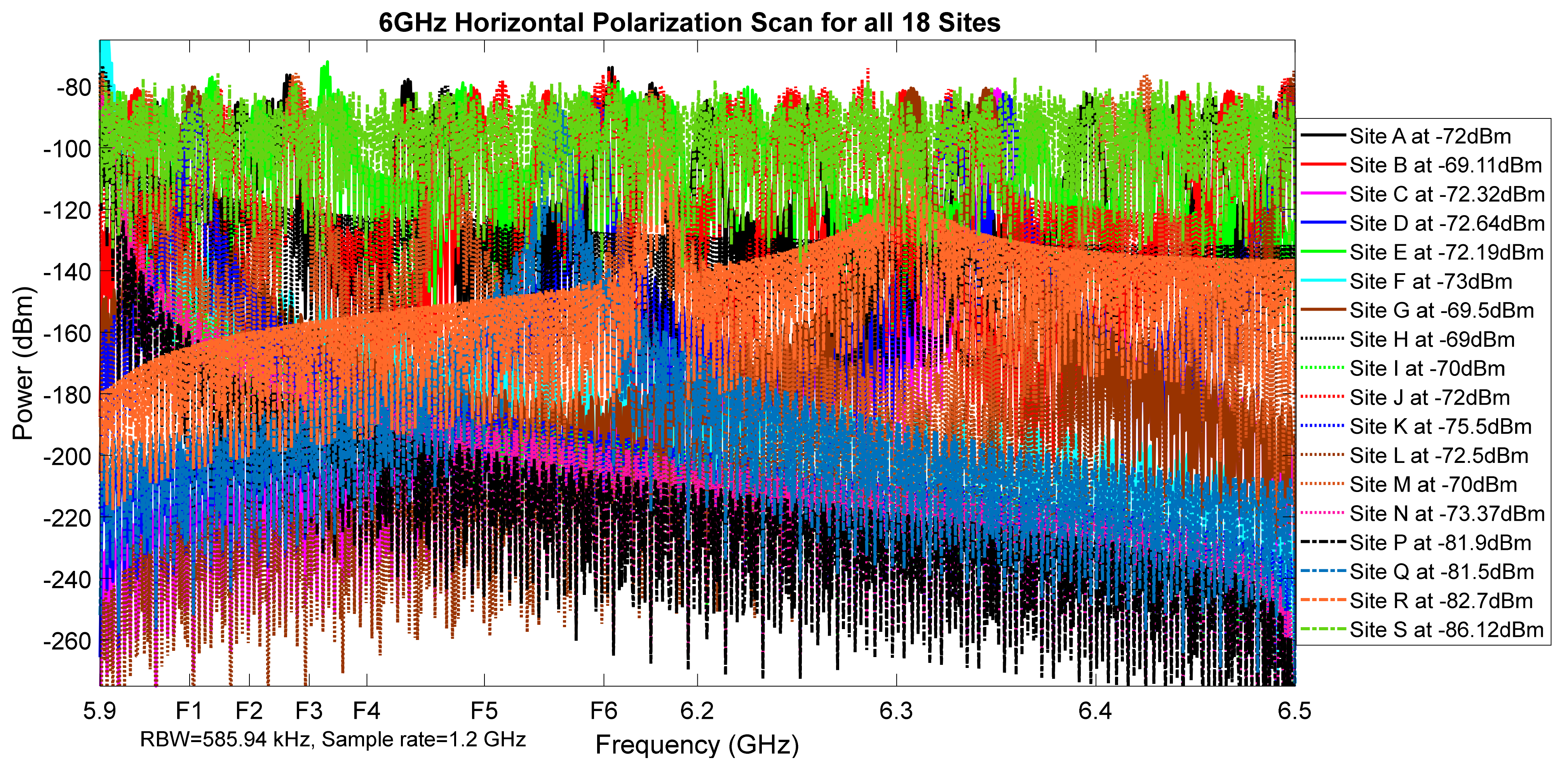
Figure 5.
6 GHz horizontal polarization scan for all 18 sites.
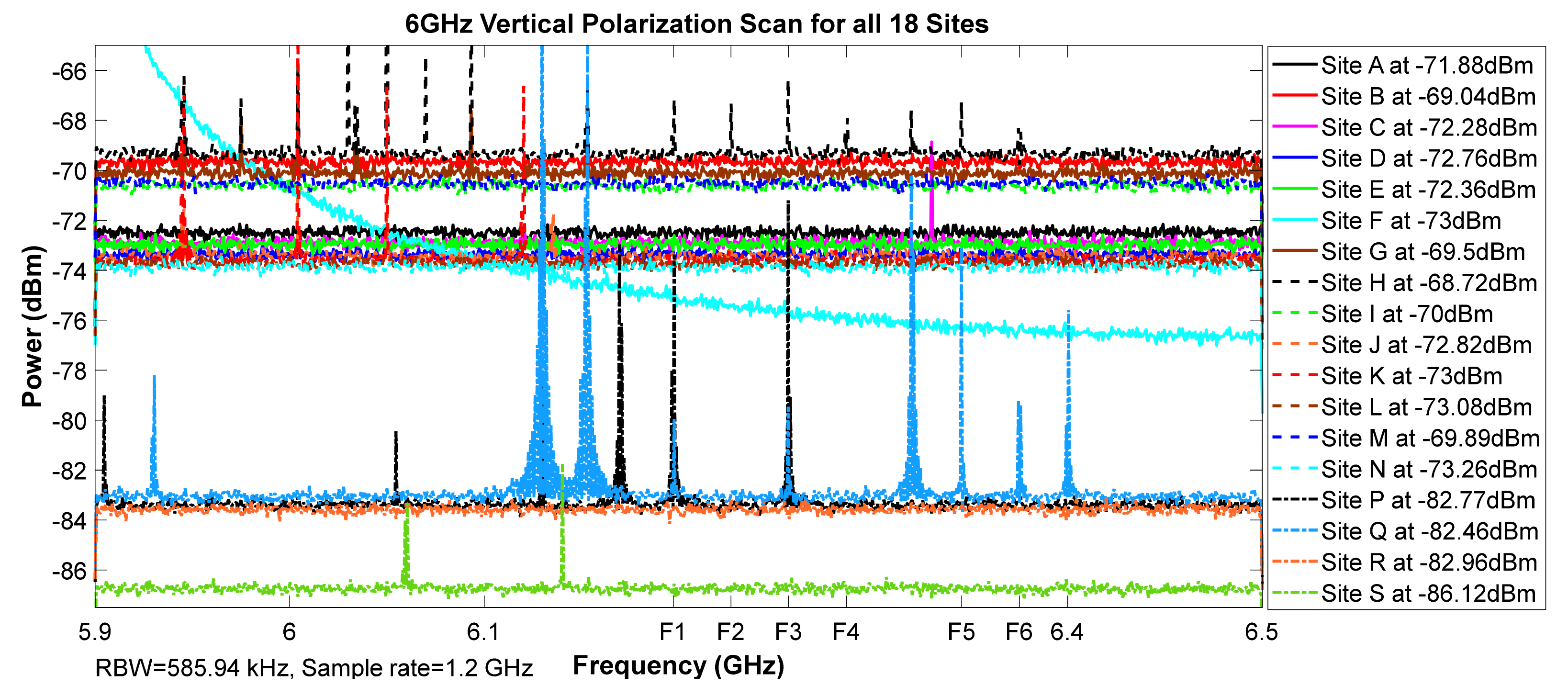
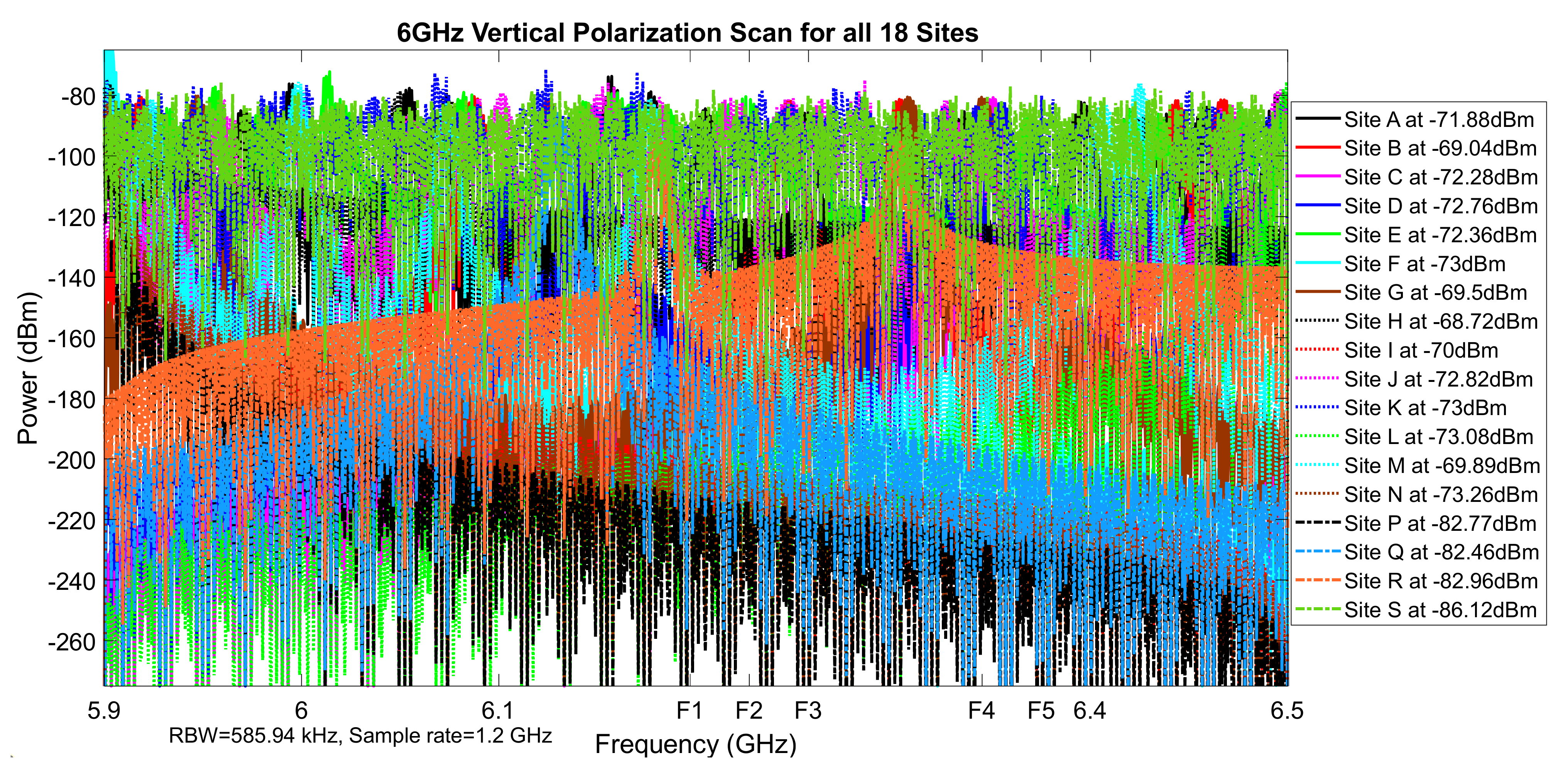
Figure 6.
6 GHz vertical polarization scan for all 18 sites.
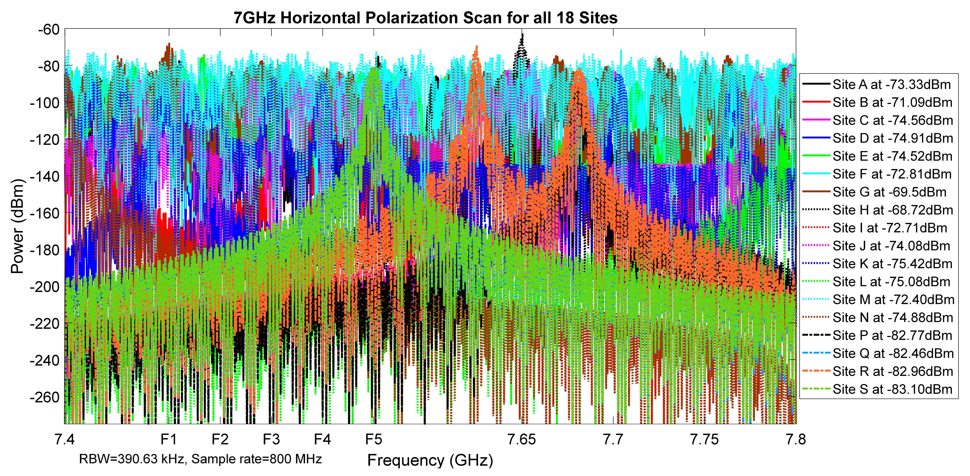
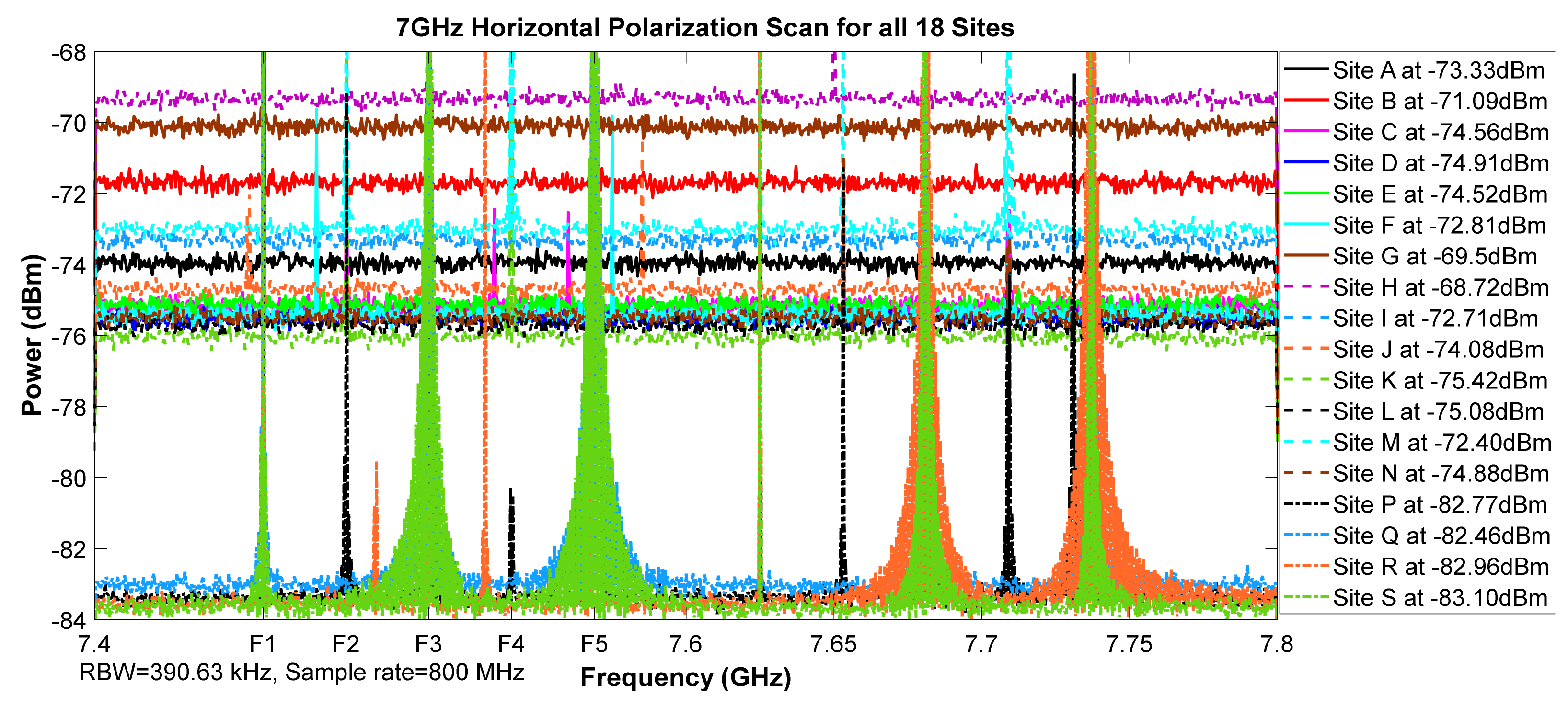
Figure 7.
7 GHz horizontal polarization scan for all 18 sites.
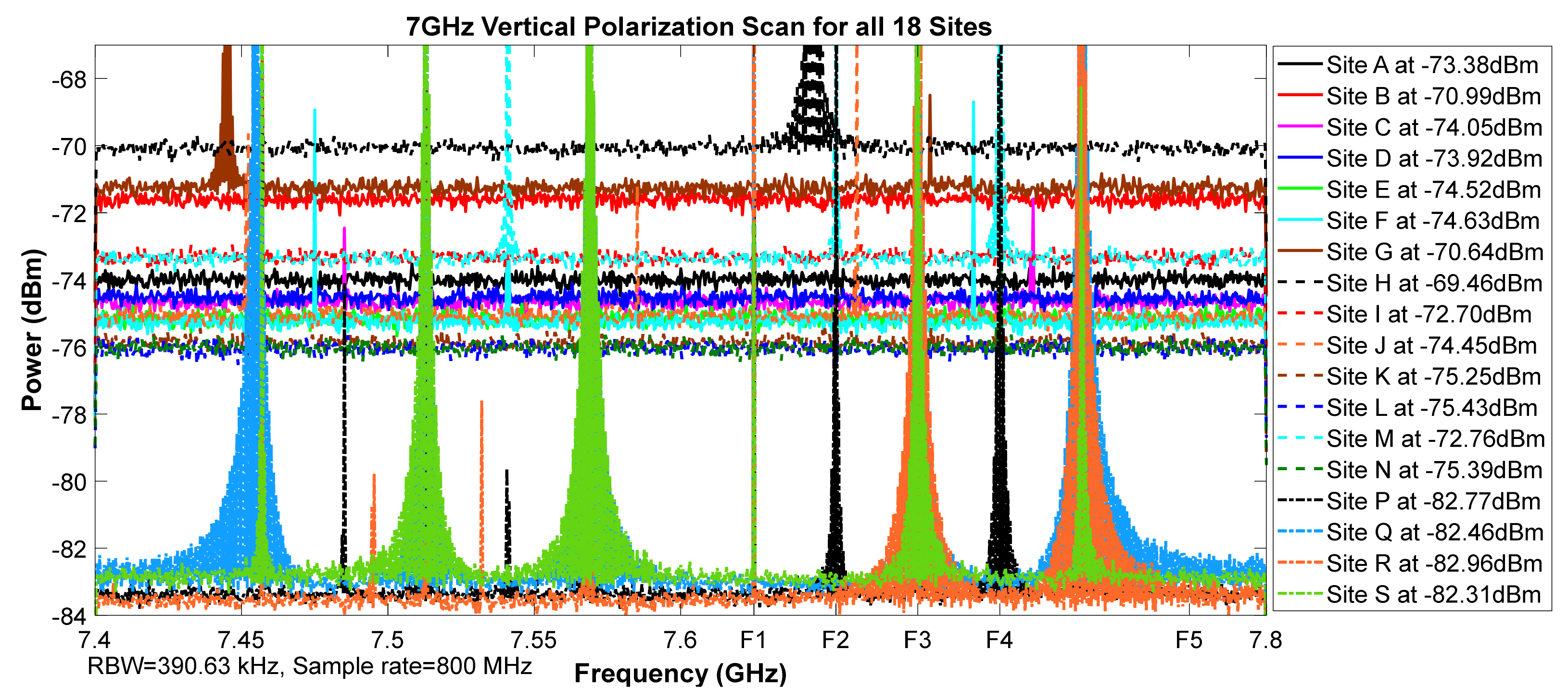
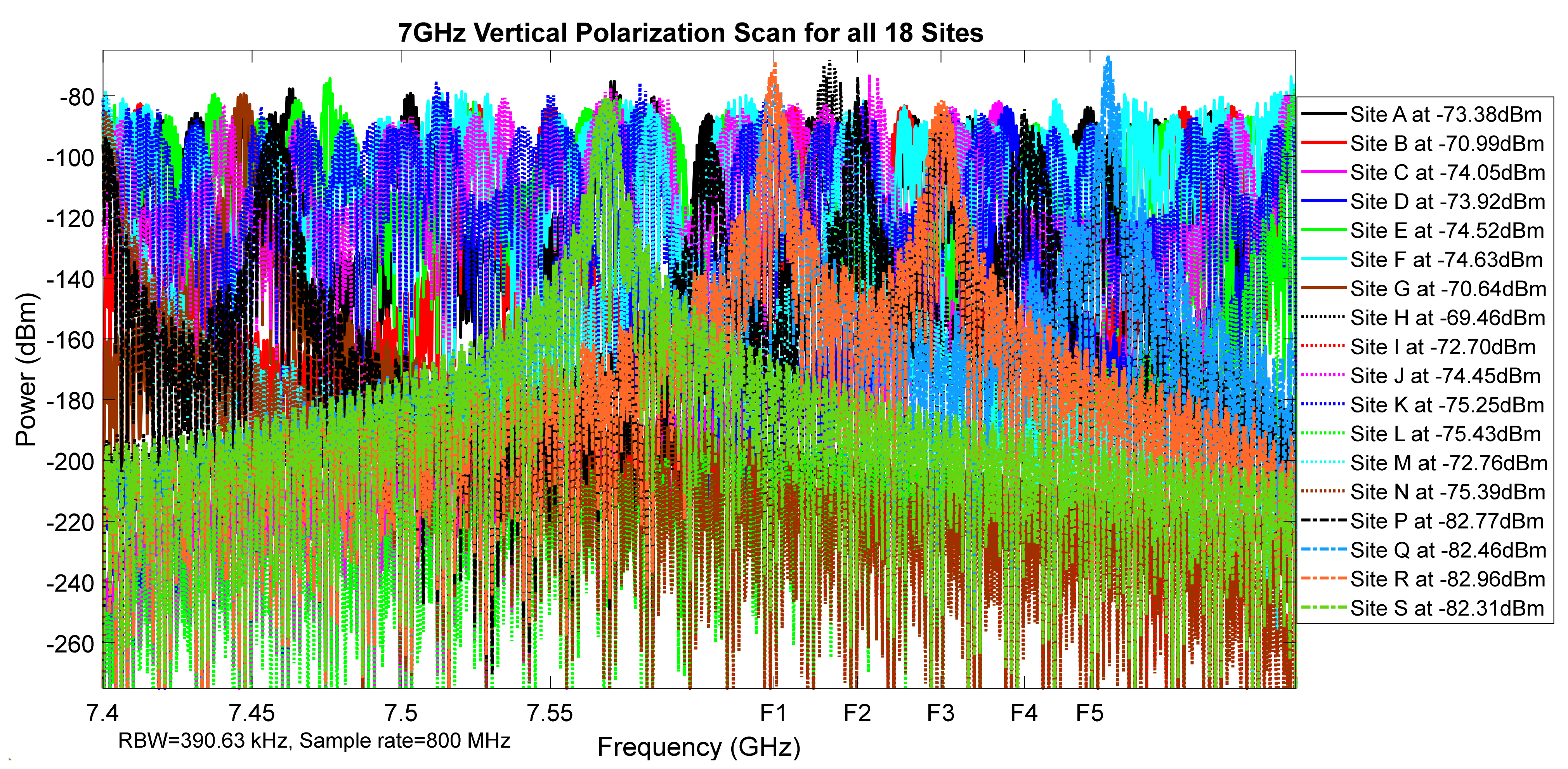
Figure 8.
7 GHz vertical polarization scan for all 18 sites.
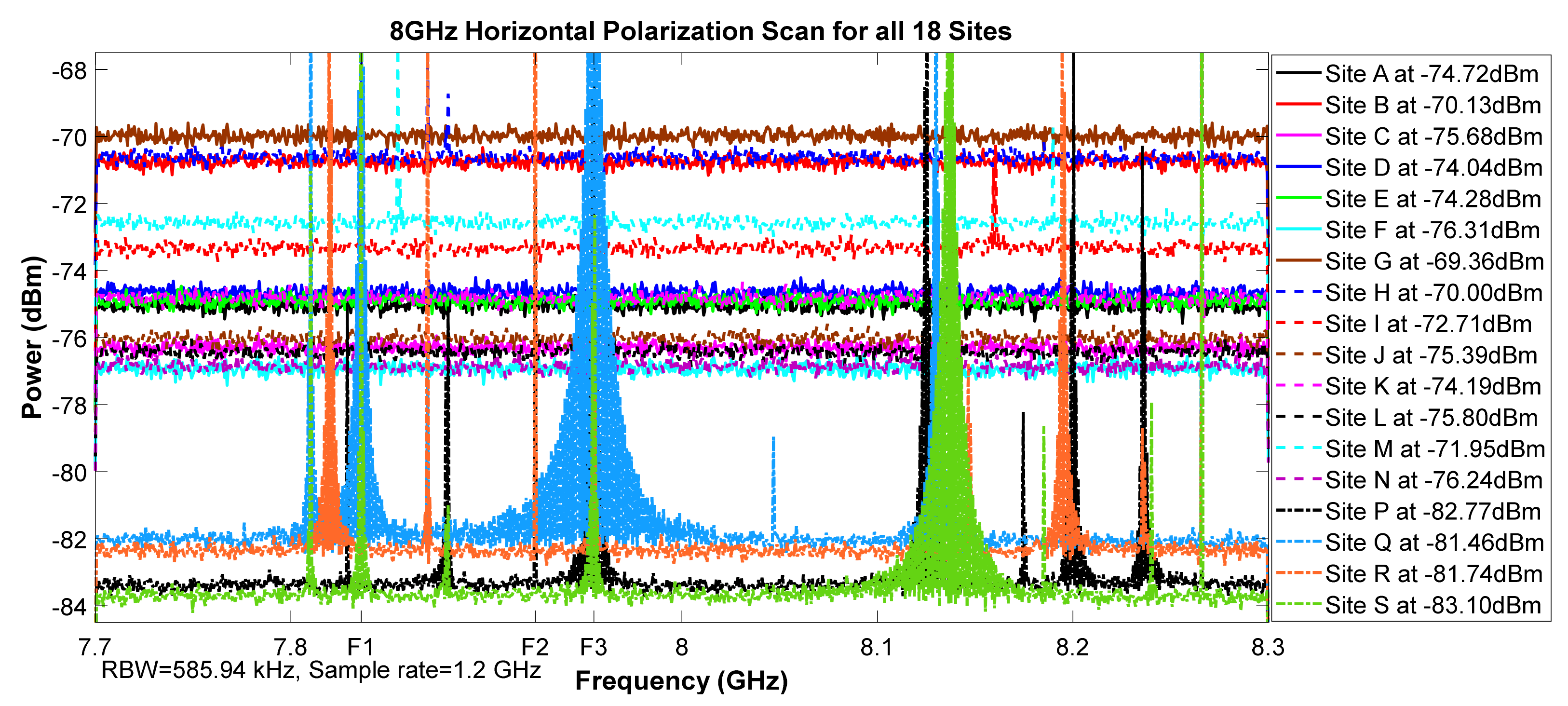
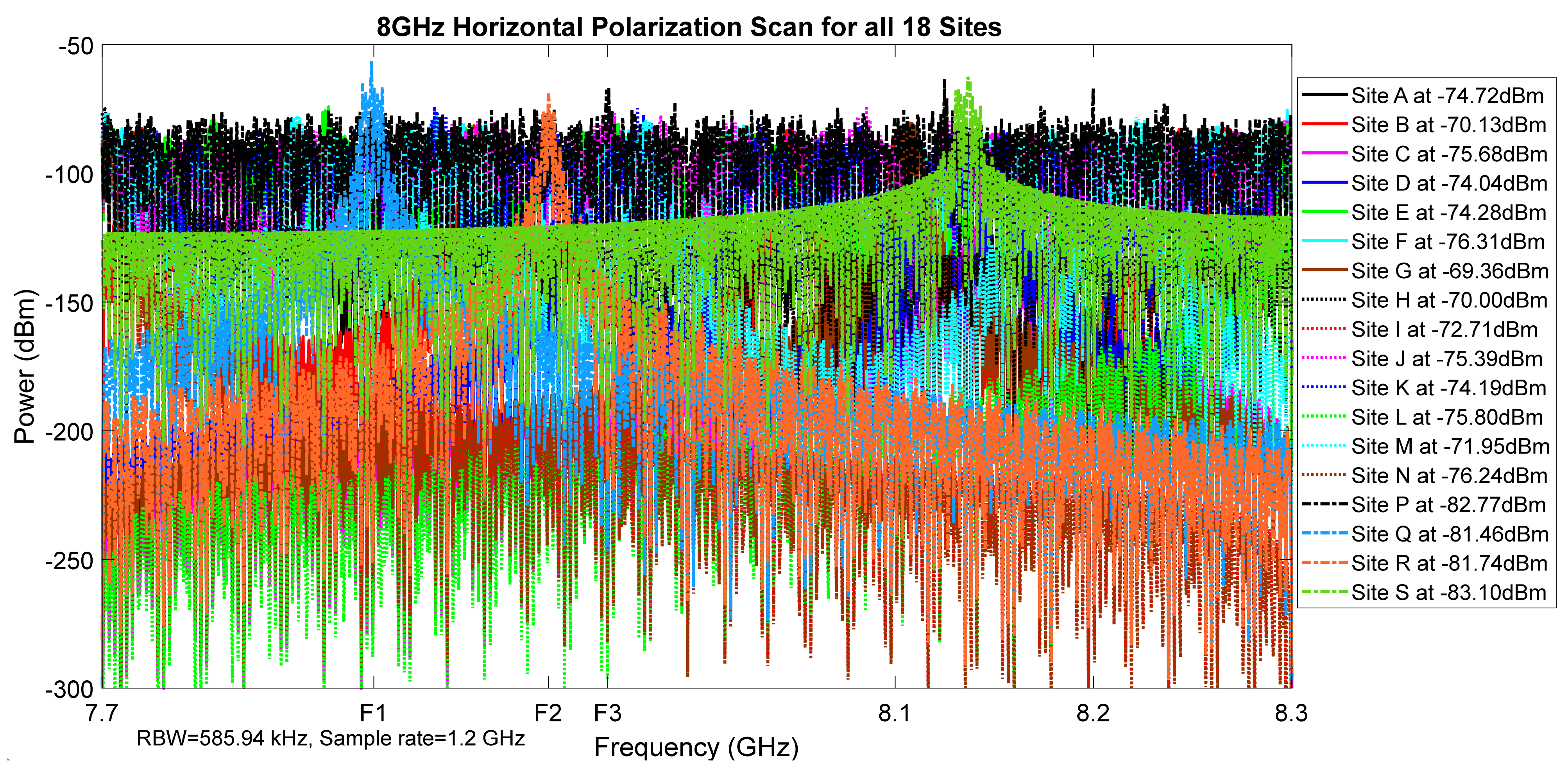
Figure 9.
8 GHz horizontal polarization scan for all 18 sites.
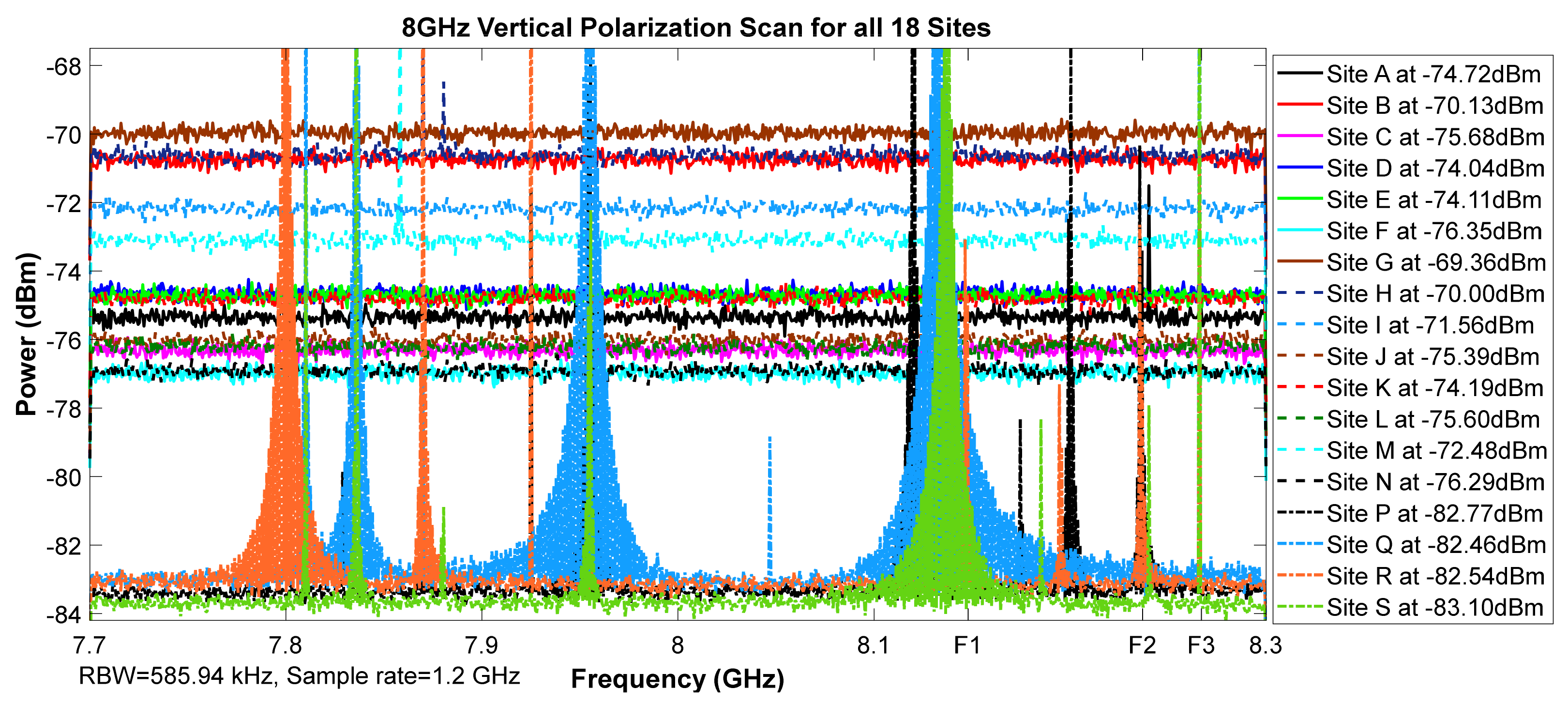
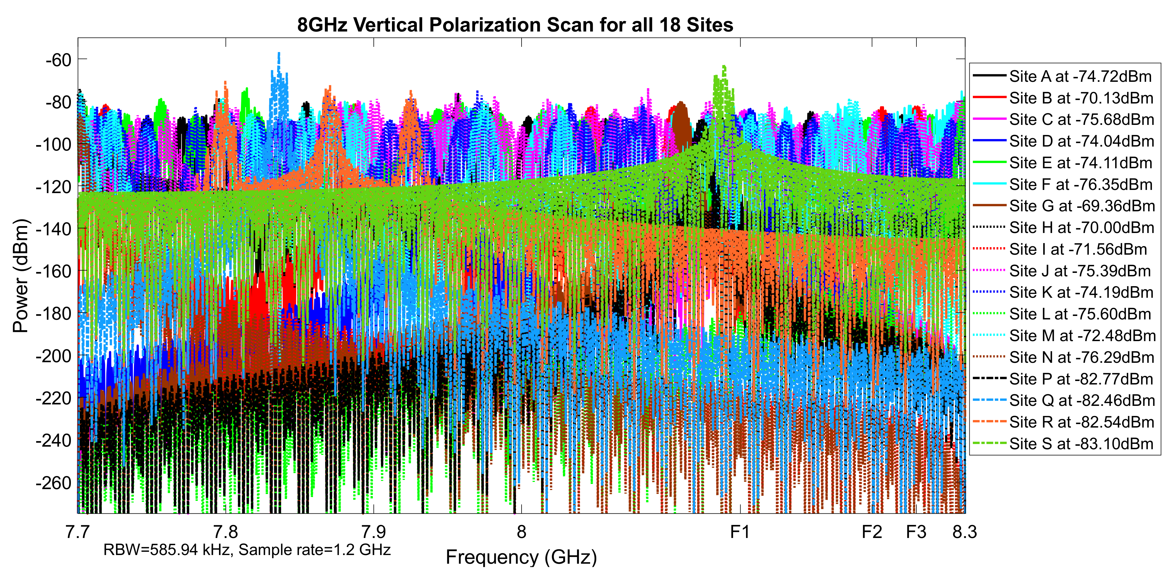
Figure 10.
8 GHz vertical polarization scan for all 18 sites.
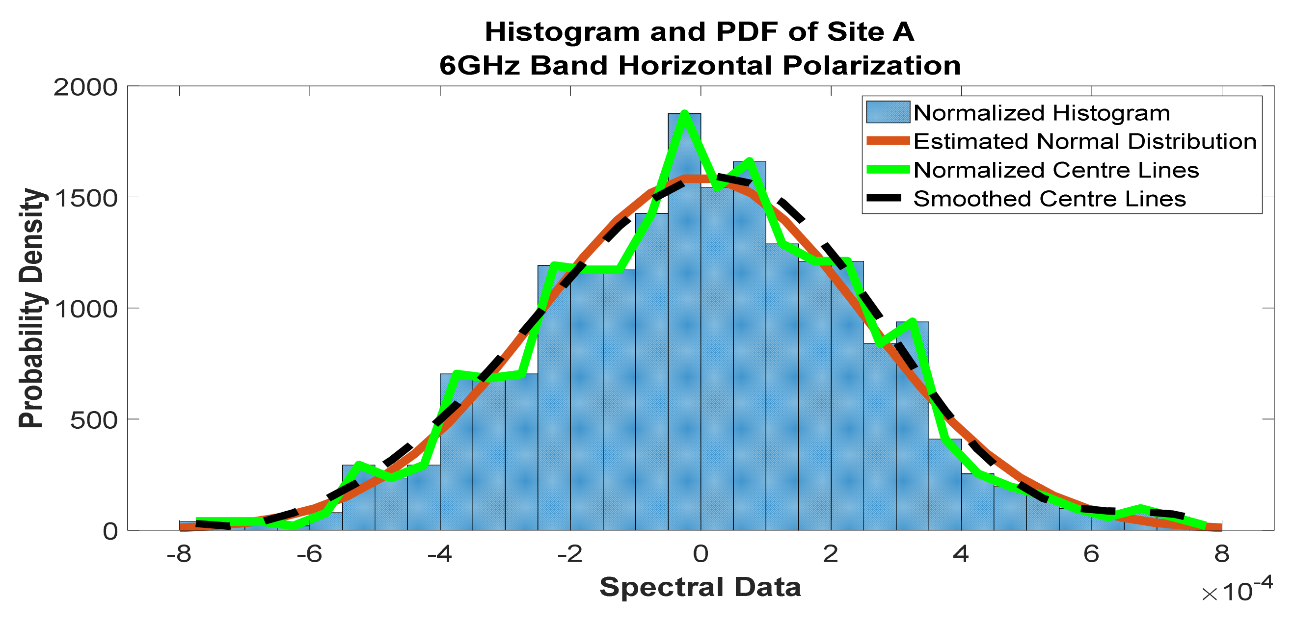
Figure 11.
Histogram and PDF of the frequency scan for site A at 6 GHz horizontal polarization.
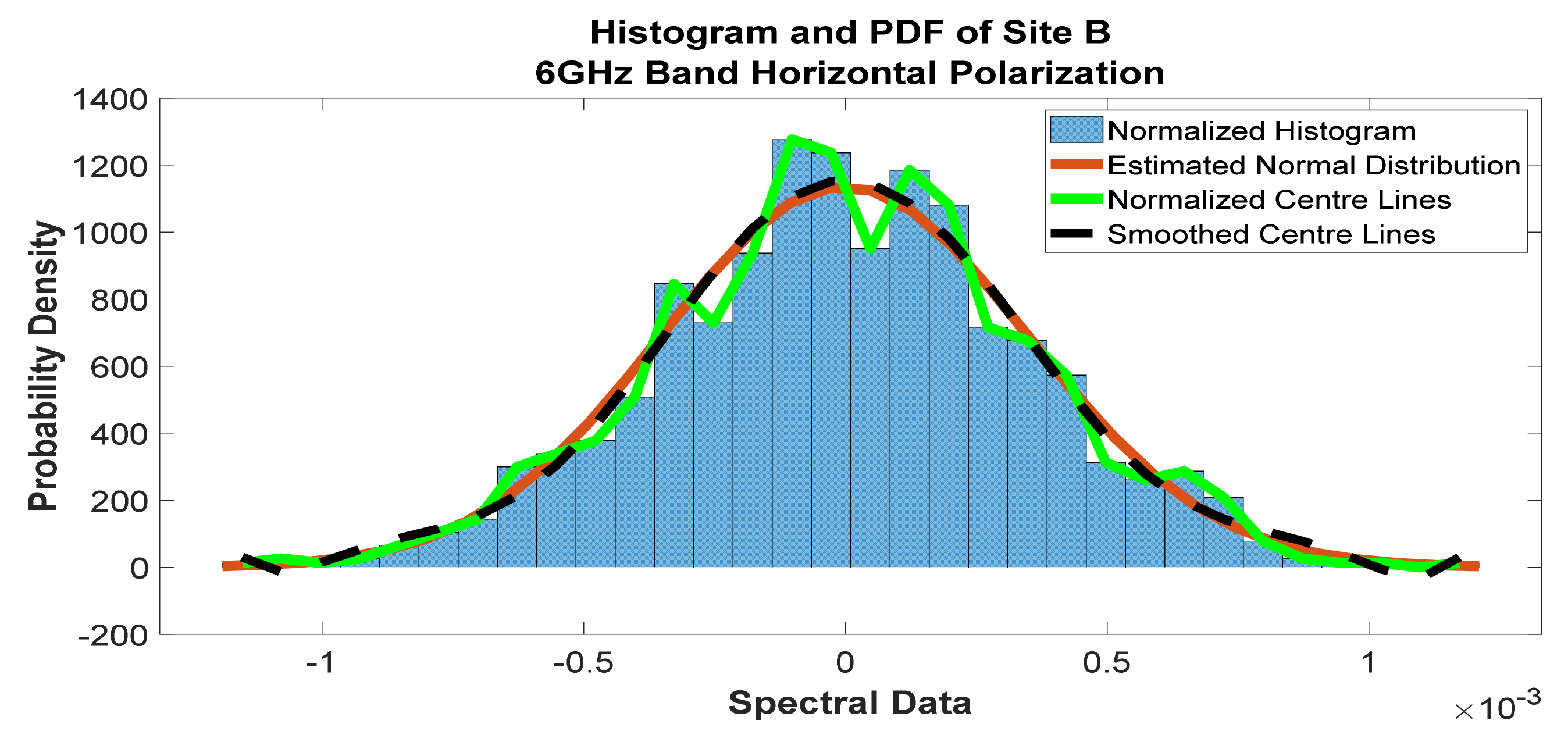
Figure 12.
Histogram and PDF of the frequency scan for site B at 6 GHz horizontal polarization.
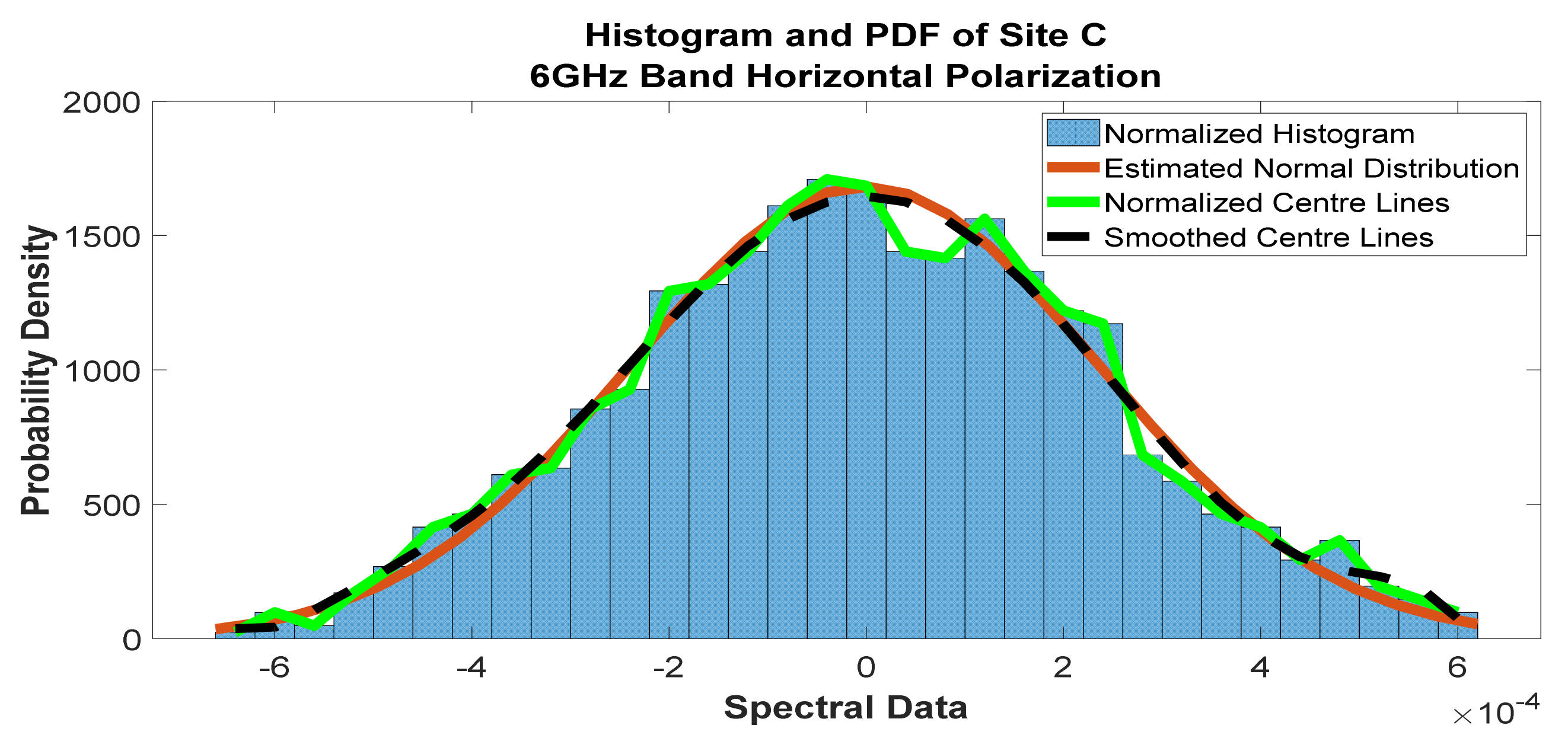
Figure 13.
Histogram and PDF of the frequency scan for site C at 6 GHz horizontal polarization.
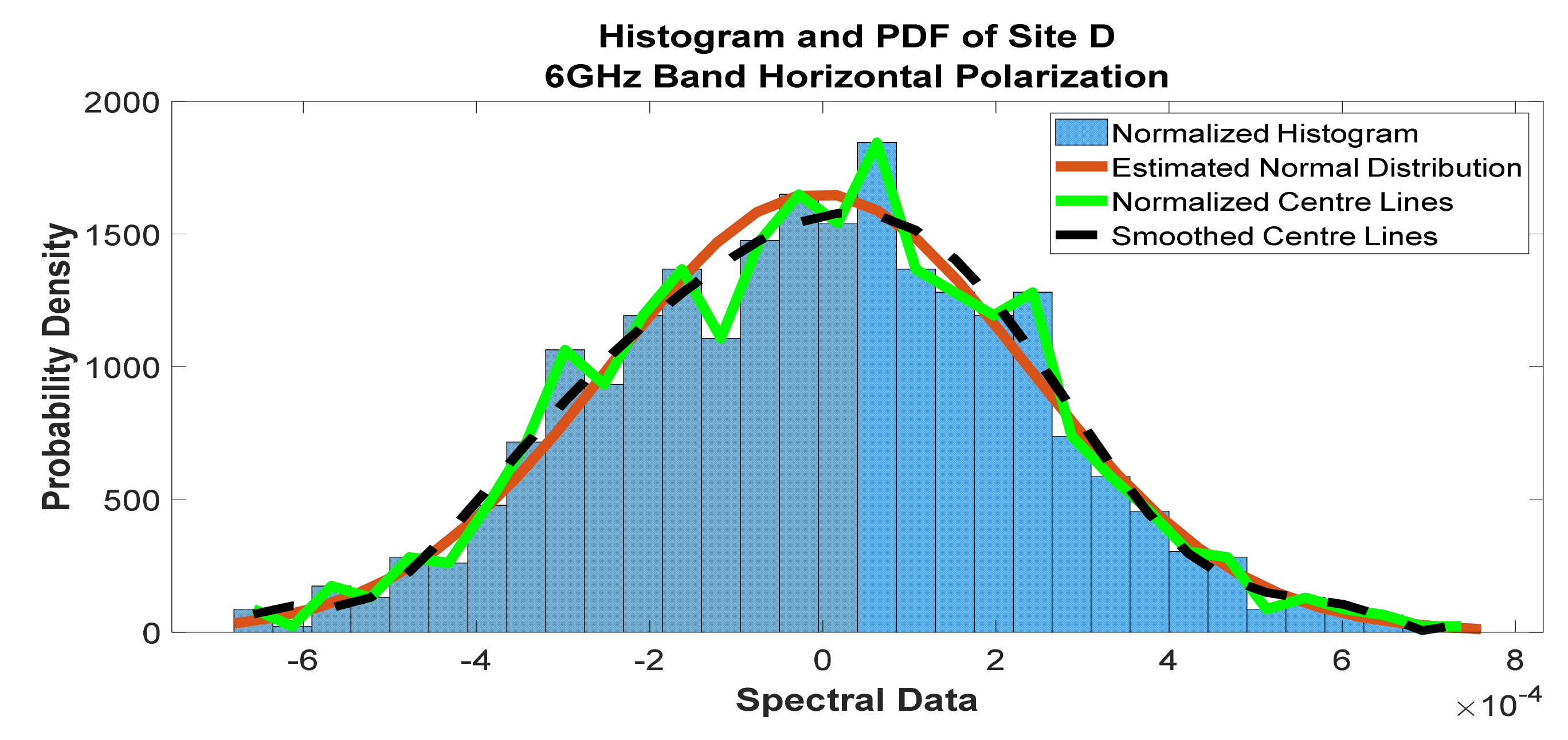
Figure 14.
Histogram and PDF of the frequency scan for site D at 6 GHz horizontal polarization.
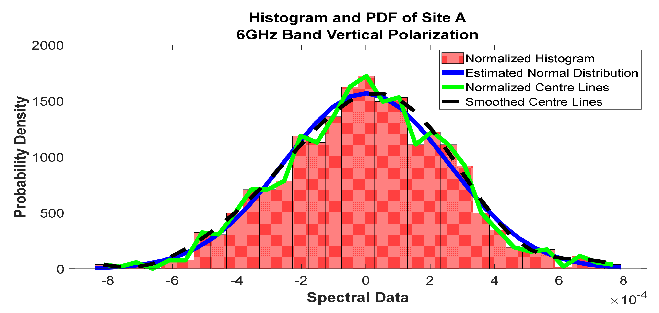
Figure 15.
Histogram and PDF of the frequency scan for site A at 6 GHz vertical polarization.
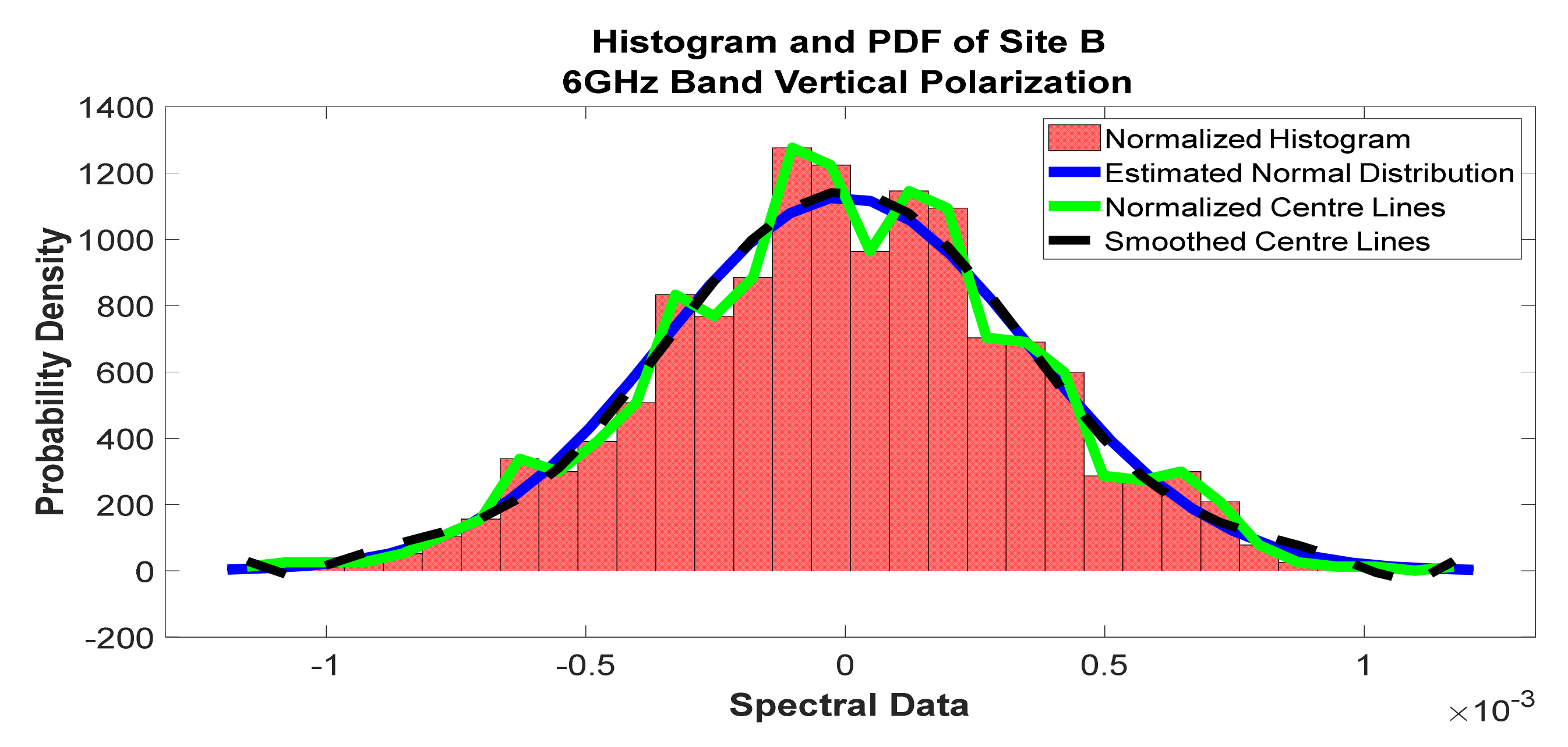
Figure 16.
Histogram and PDF of the frequency scan for site B at 6 GHz vertical polarization.
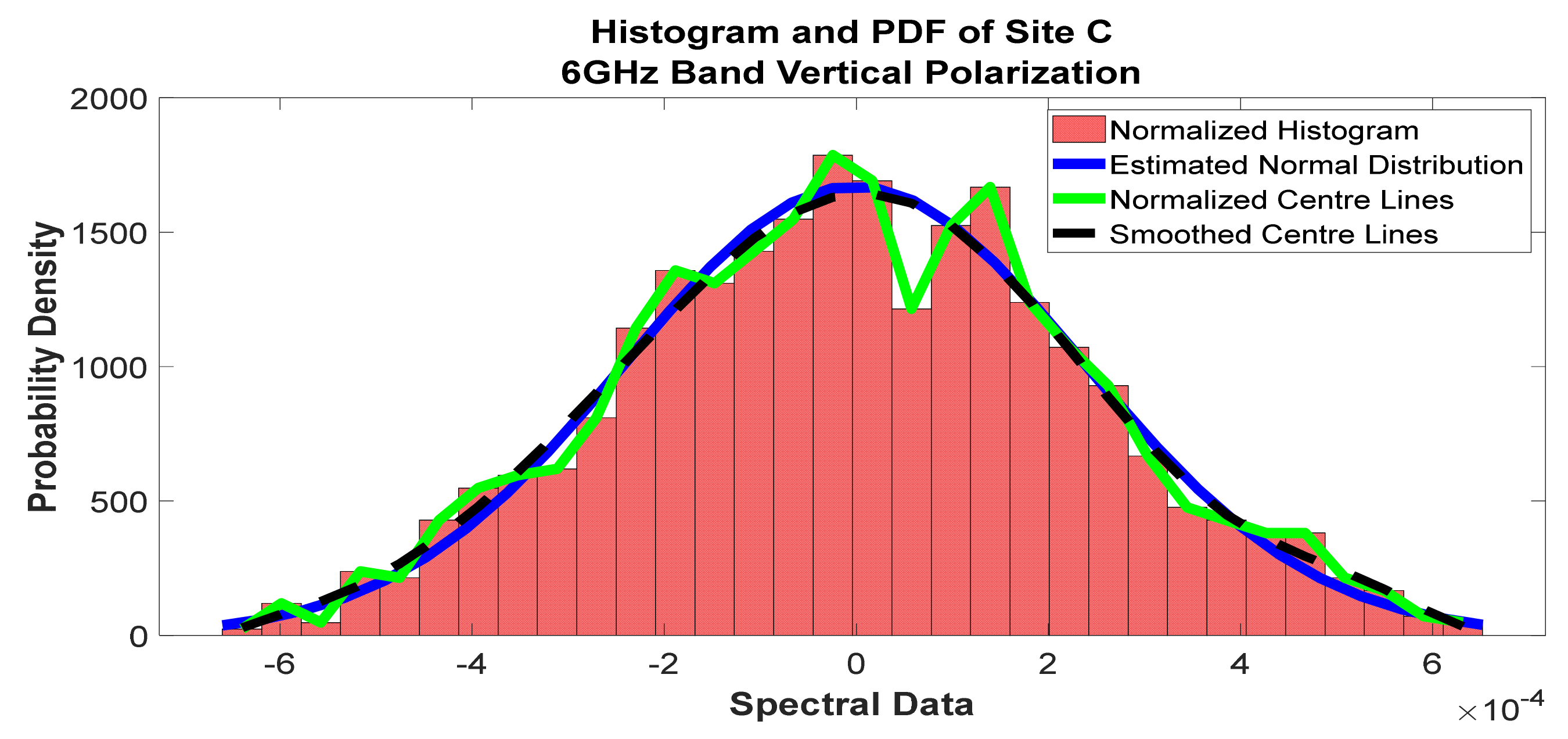
Figure 17.
Histogram and PDF of the frequency scan for site C at 6 GHz vertical polarization.
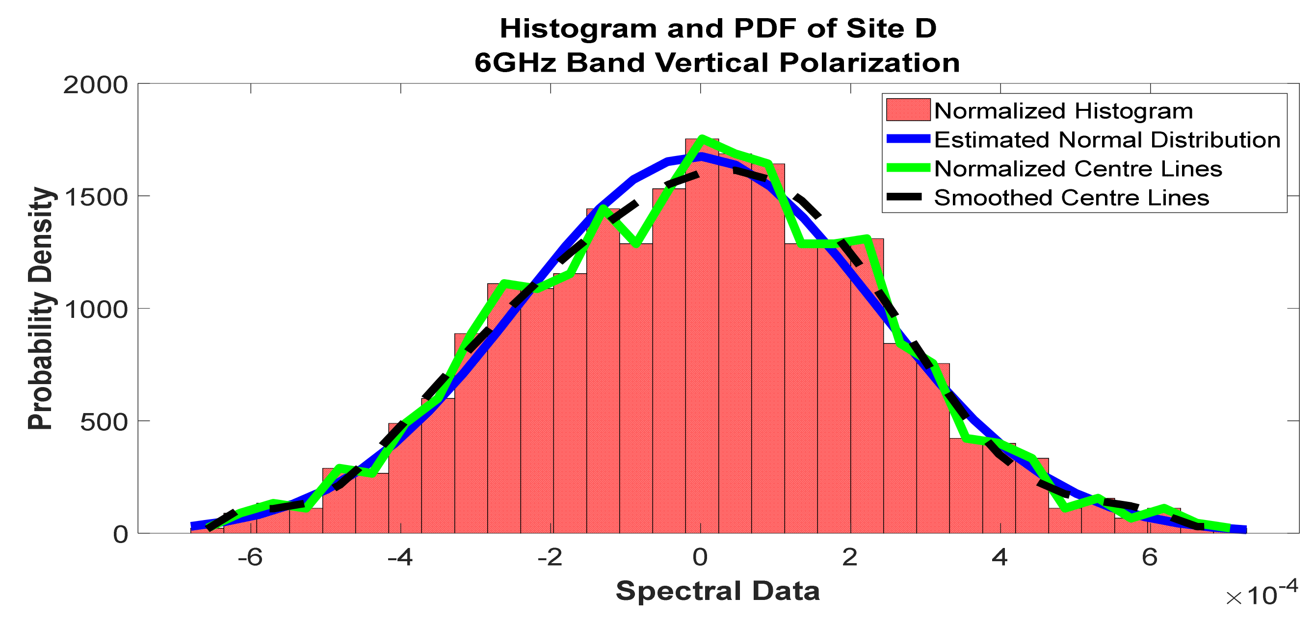
Figure 18.
Histogram and PDF of the frequency scan for site D at 6 GHz vertical polarization.
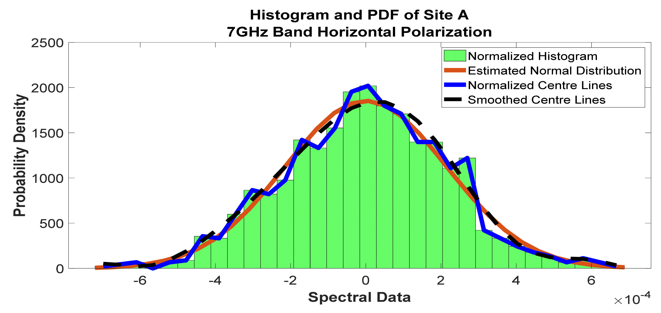
Figure 19.
Histogram and PDF of the frequency scan for site A at 7 GHz horizontal polarization.
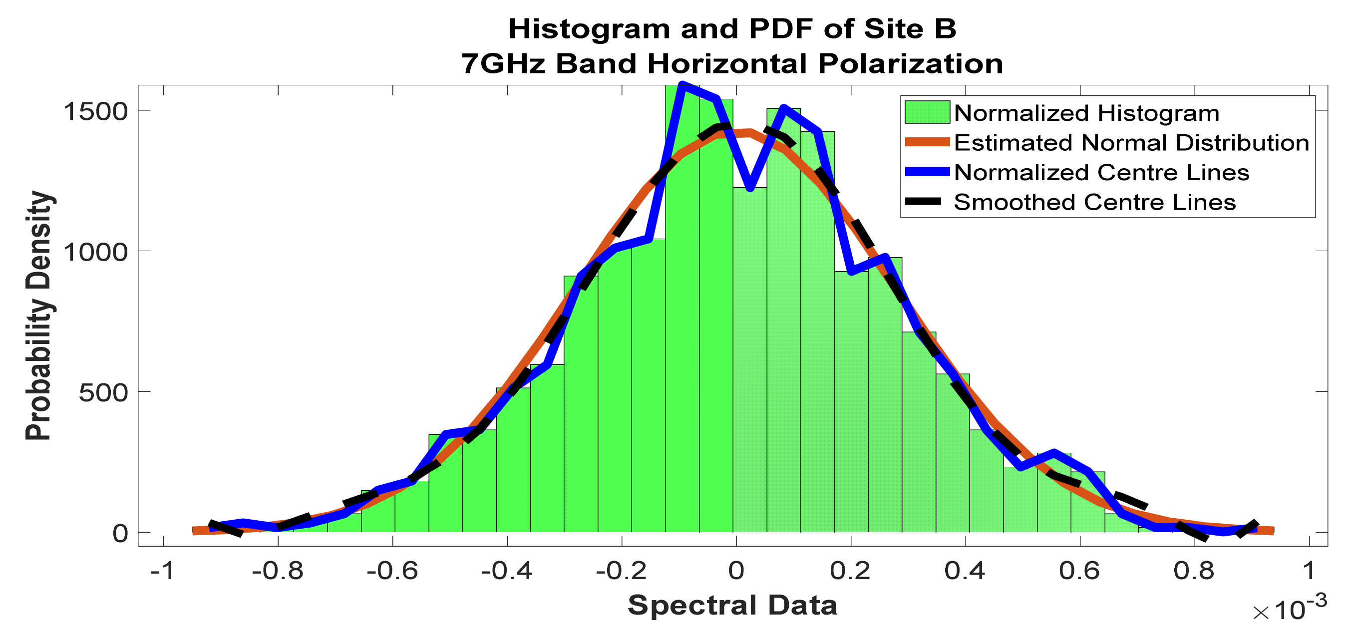
Figure 20.
Histogram and PDF of the frequency scan for site B at 7 GHz horizontal polarization.
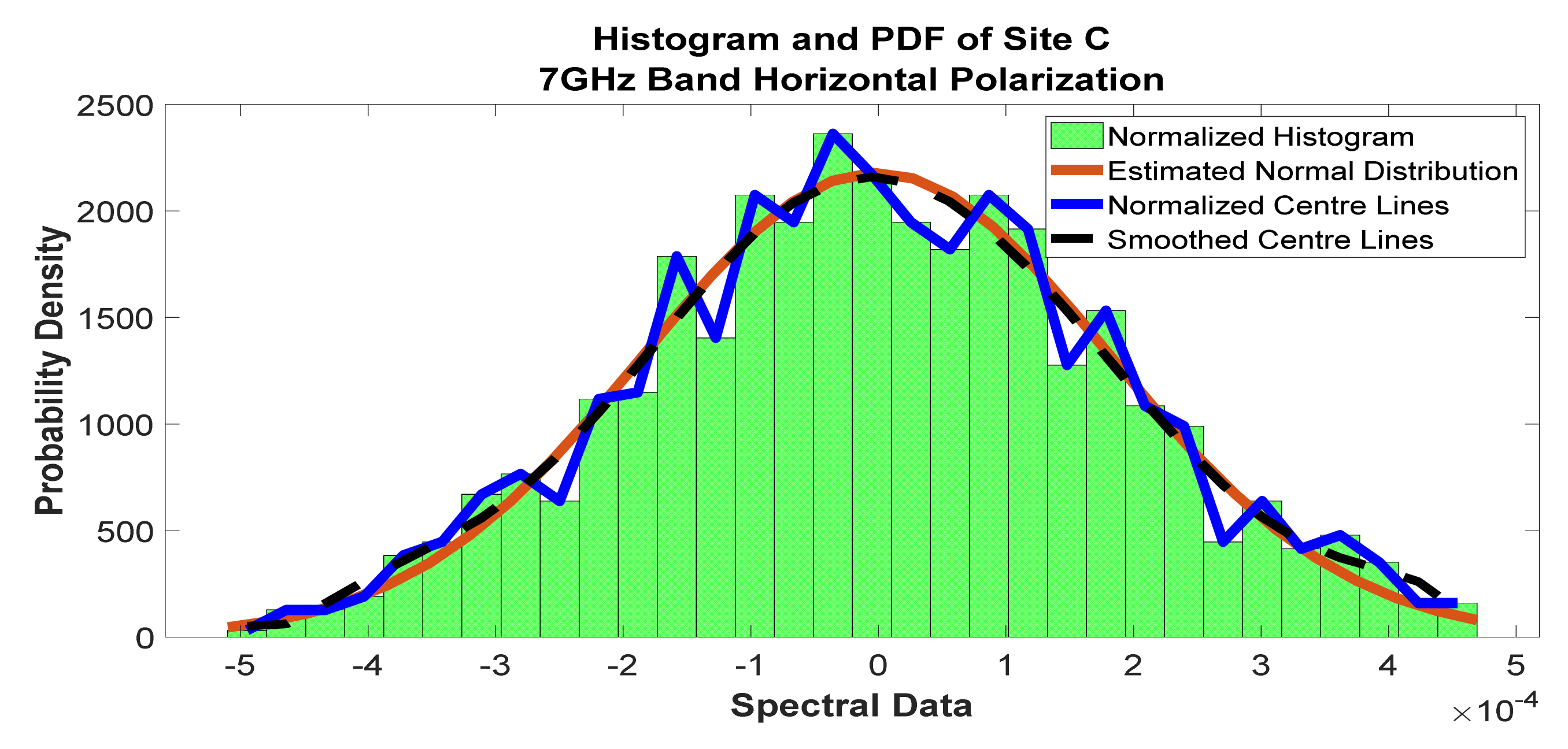
Figure 21.
Histogram and PDF of the frequency scan for site C at 7 GHz horizontal polarization.
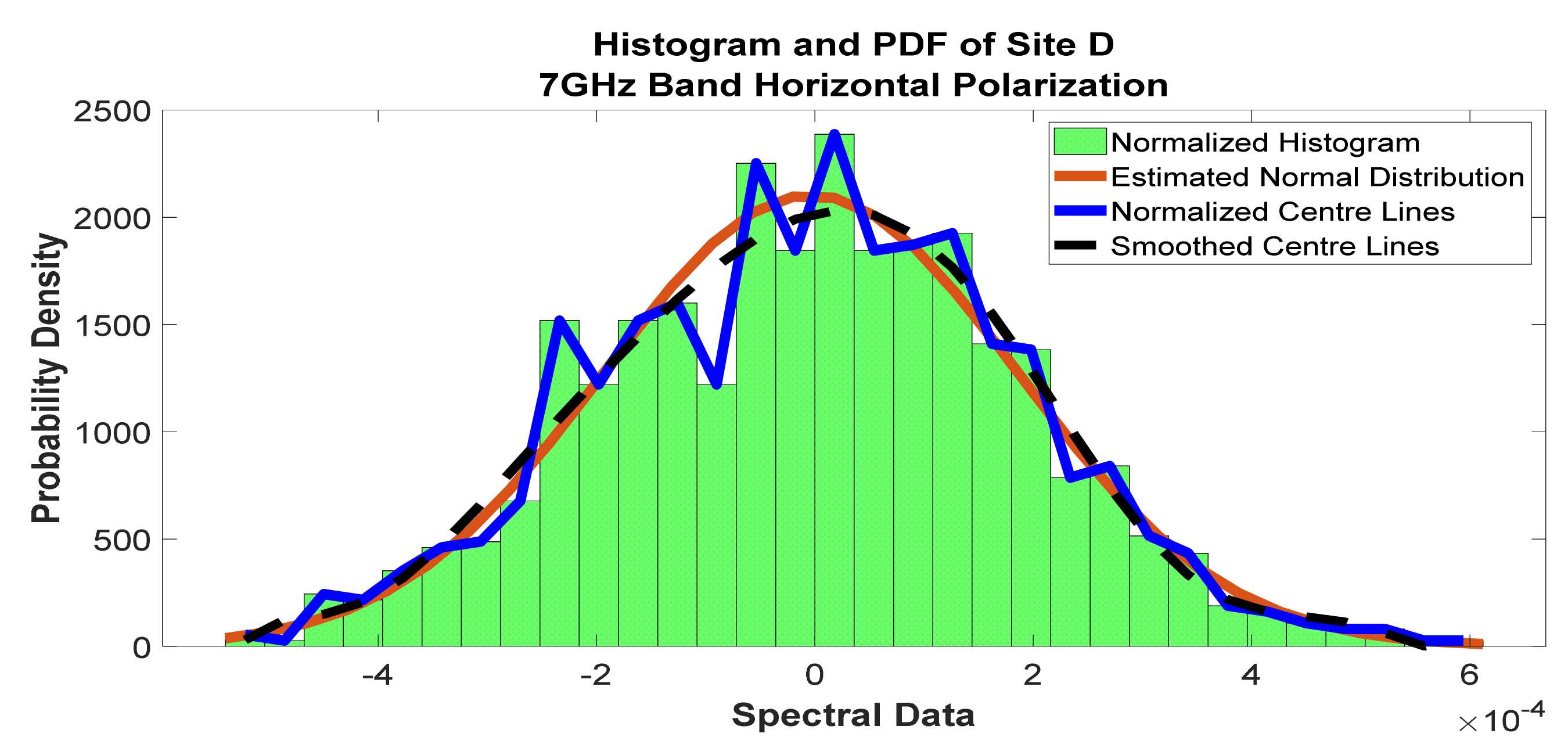
Figure 22.
Histogram and PDF of the frequency scan for site D at 7 GHz horizontal polarization.
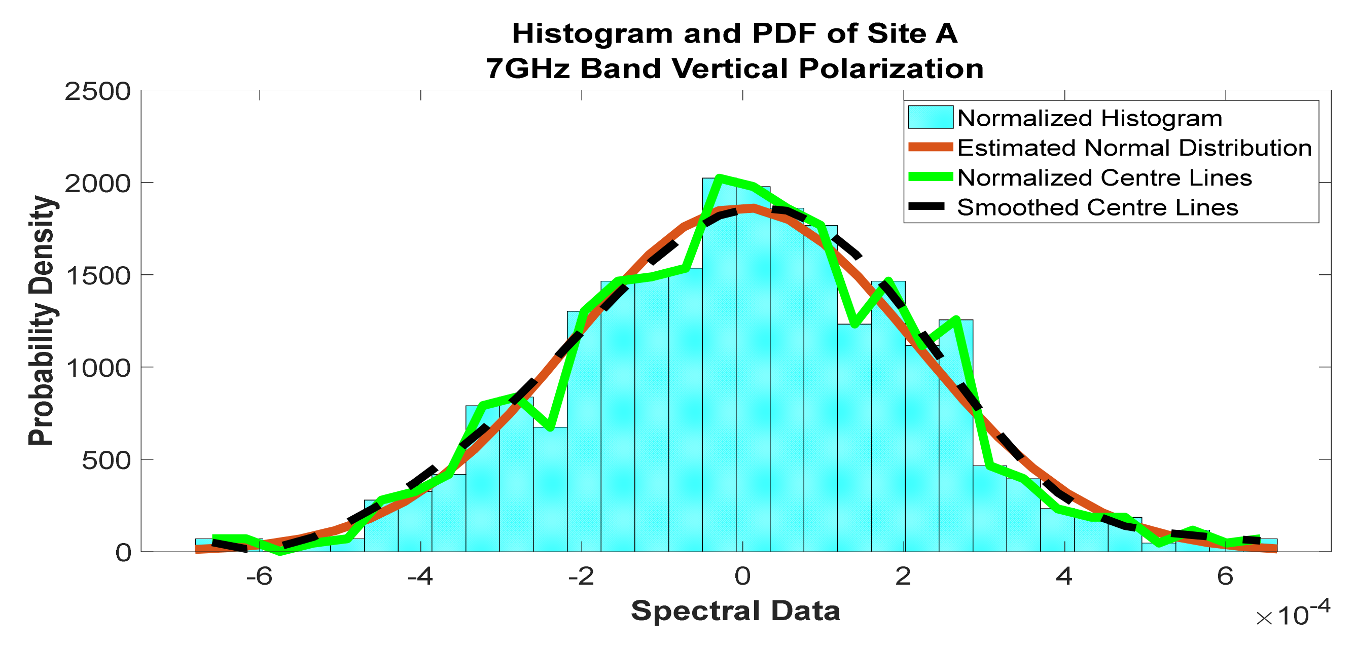
Figure 23.
Histogram and PDF of the frequency scan for site A at 7 GHz vertical polarization.
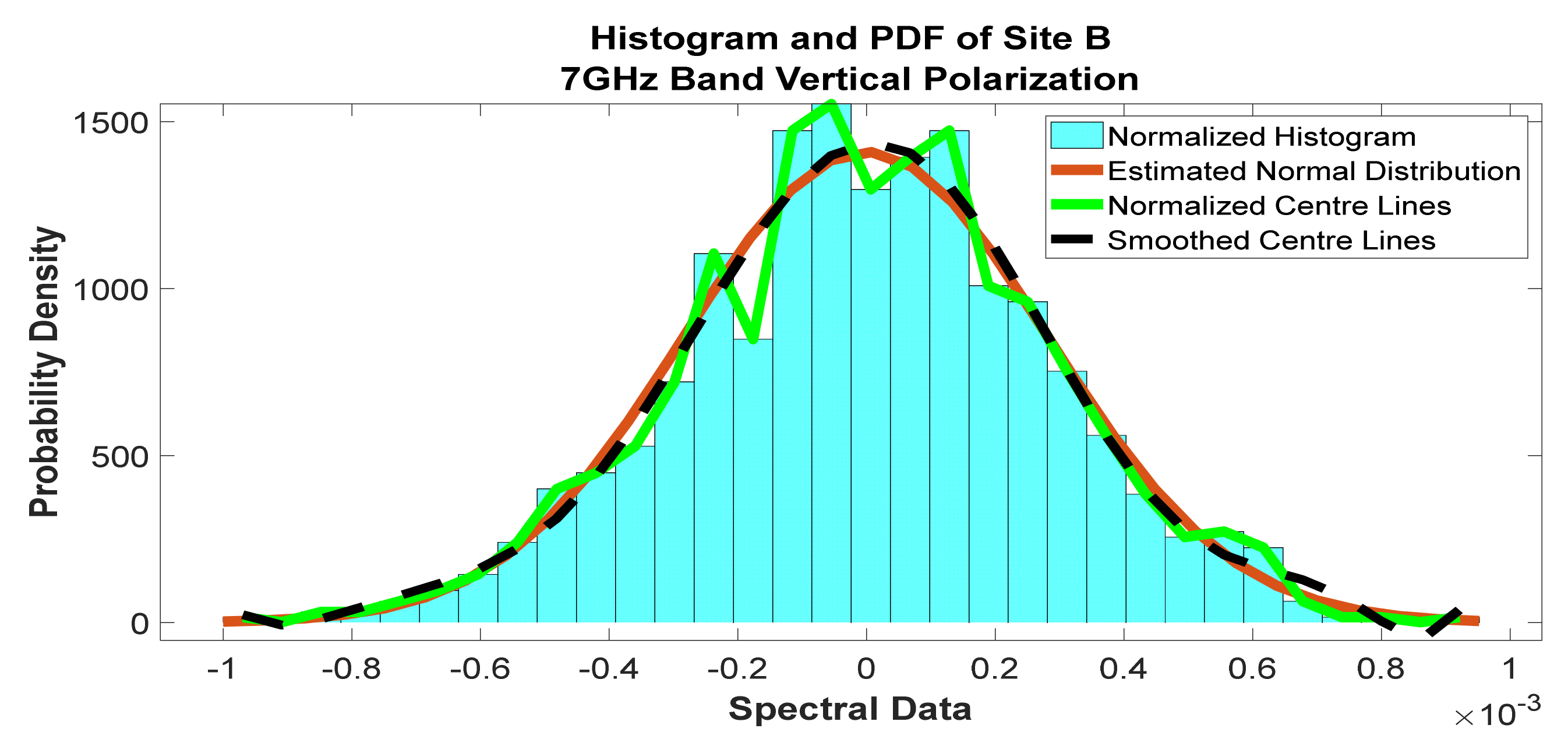
Figure 24.
Histogram and PDF of the frequency scan for site B at 7 GHz vertical polarization.
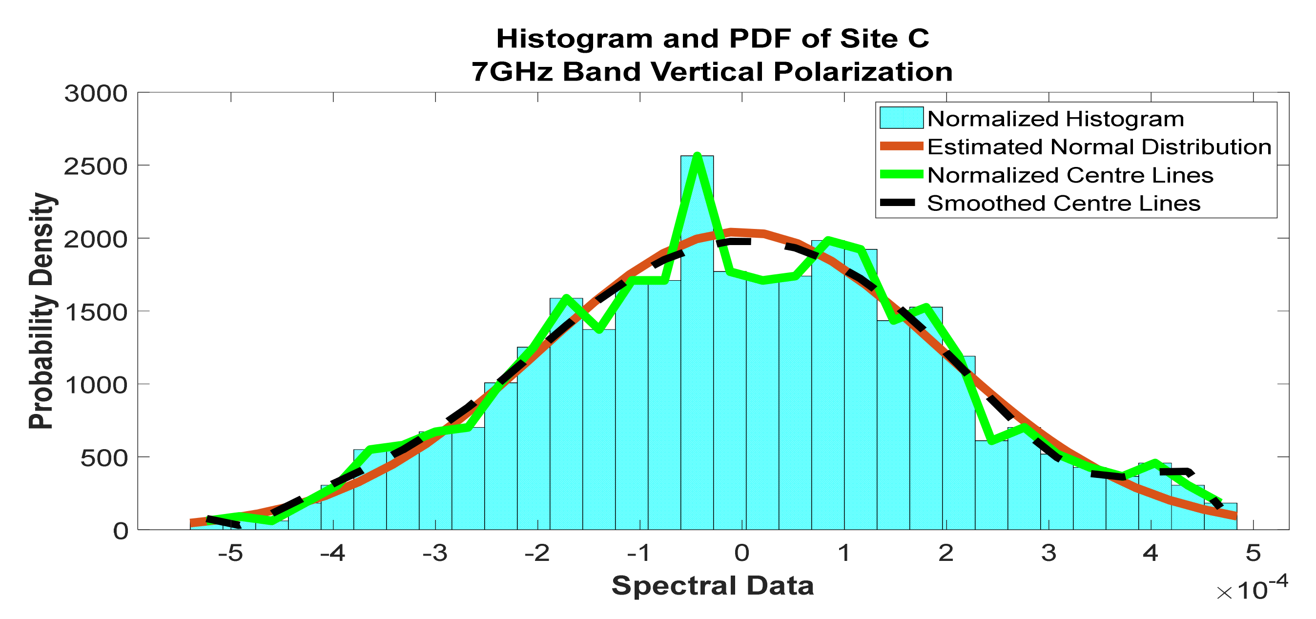
Figure 25.
Histogram and PDF of the frequency scan for site C at 7 GHz vertical polarization.
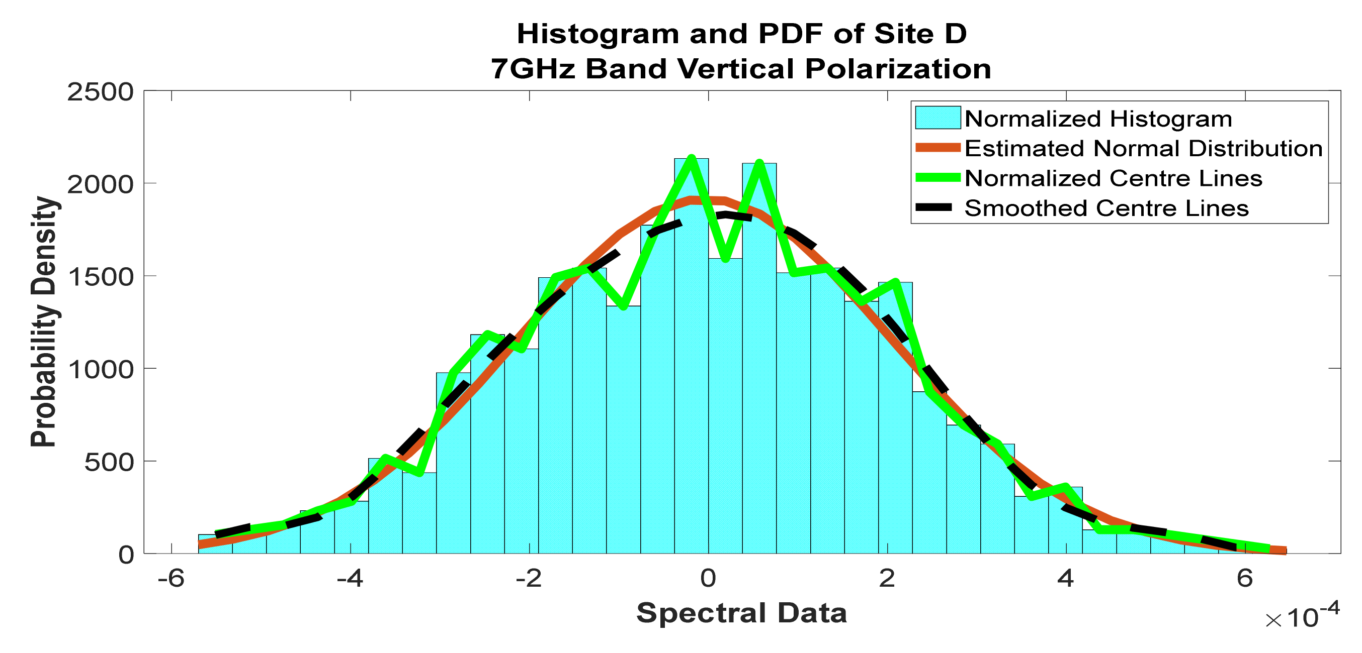
Figure 26.
Histogram and PDF of the frequency scan for site D at 7 GHz vertical polarization.
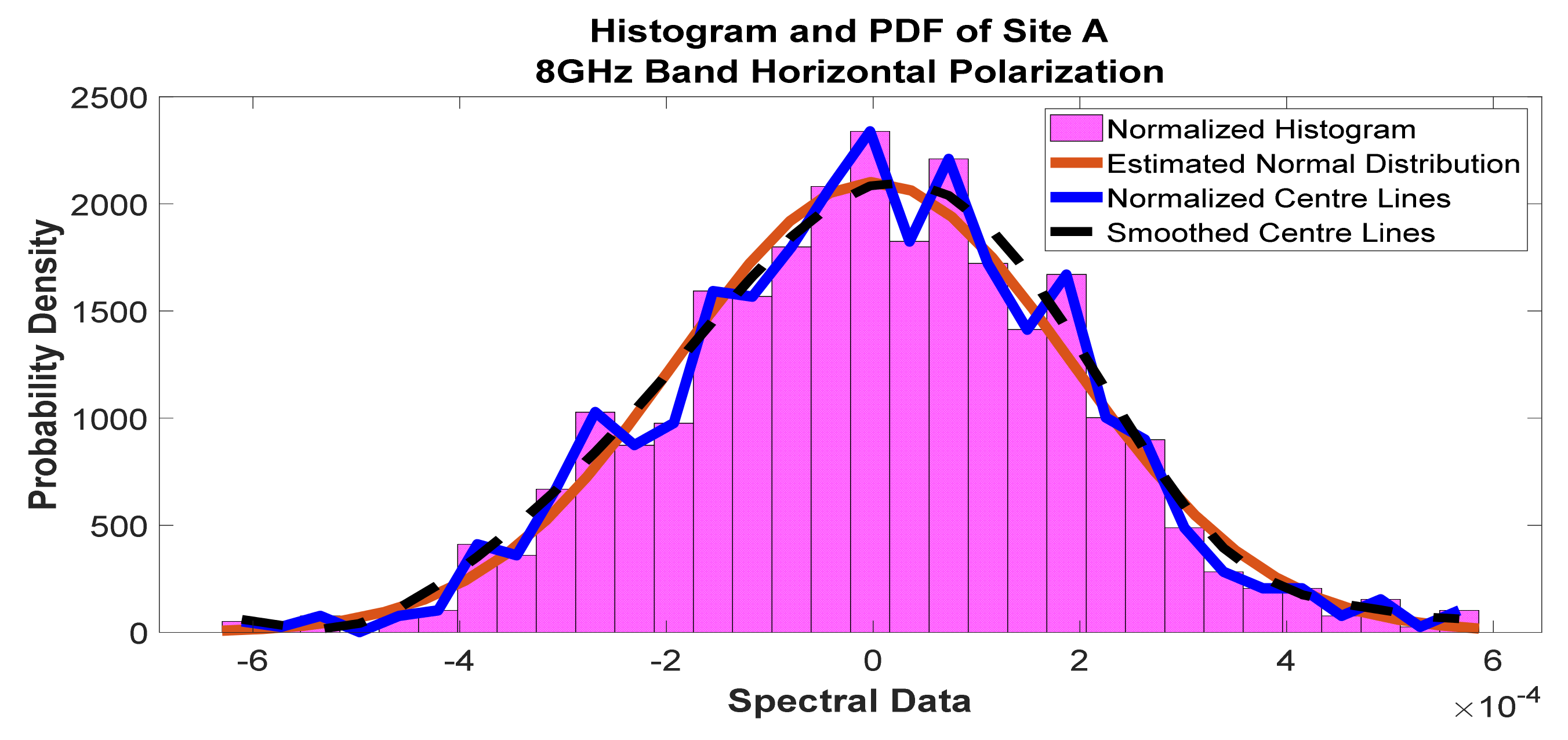
Figure 27.
Histogram and PDF of the frequency scan for site A at 8 GHz horizontal polarization.
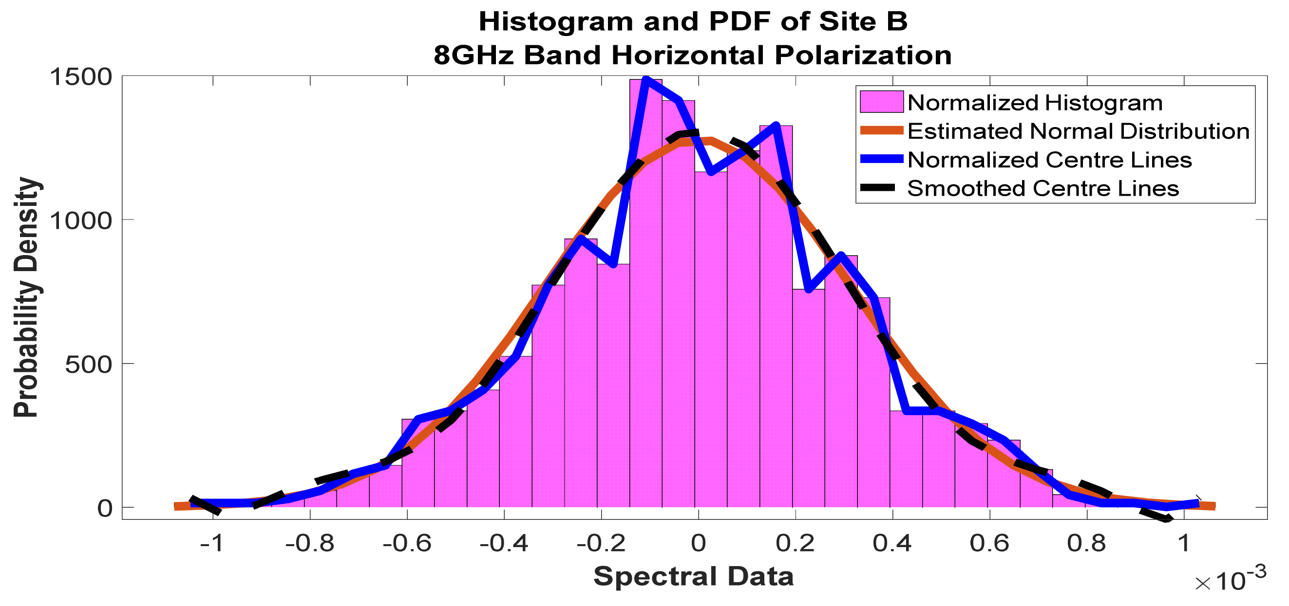
Figure 28.
Histogram and PDF of the frequency scan for site B at 8 GHz horizontal polarization.
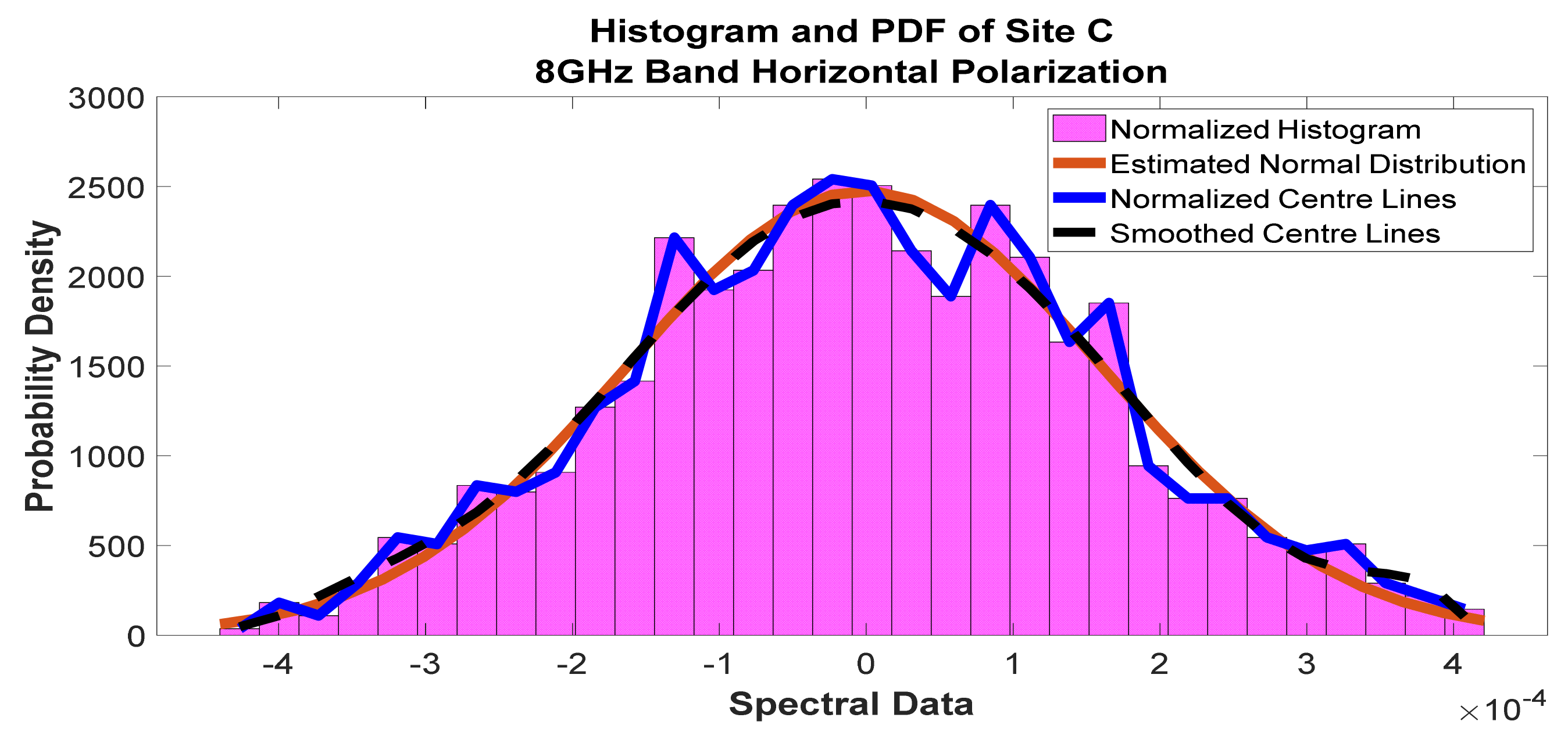
Figure 29.
Histogram and PDF of the frequency scan for site C at 8 GHz horizontal polarization.
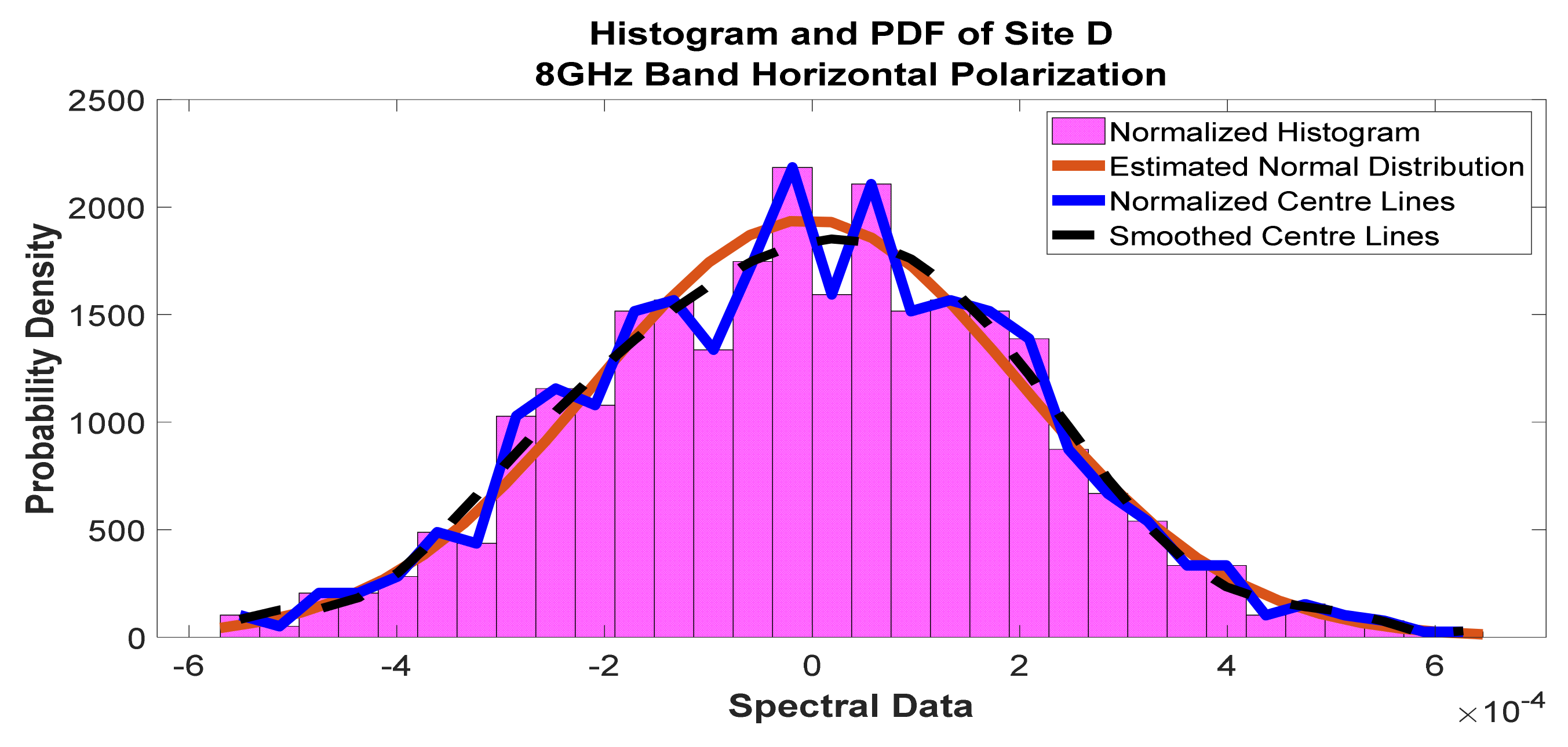
Figure 30.
Histogram and PDF of the frequency scan for site D at 8 GHz horizontal polarization.
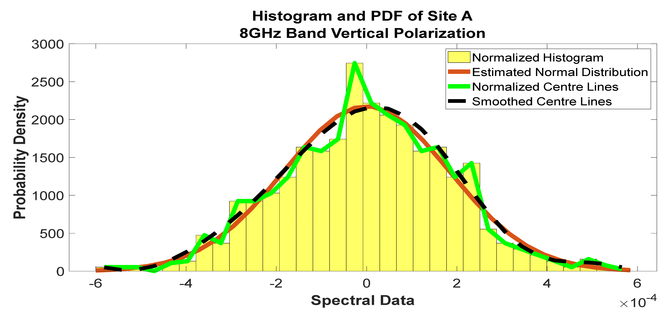
Figure 31.
Histogram and PDF of the frequency scan for site A at 8 GHz vertical polarization.
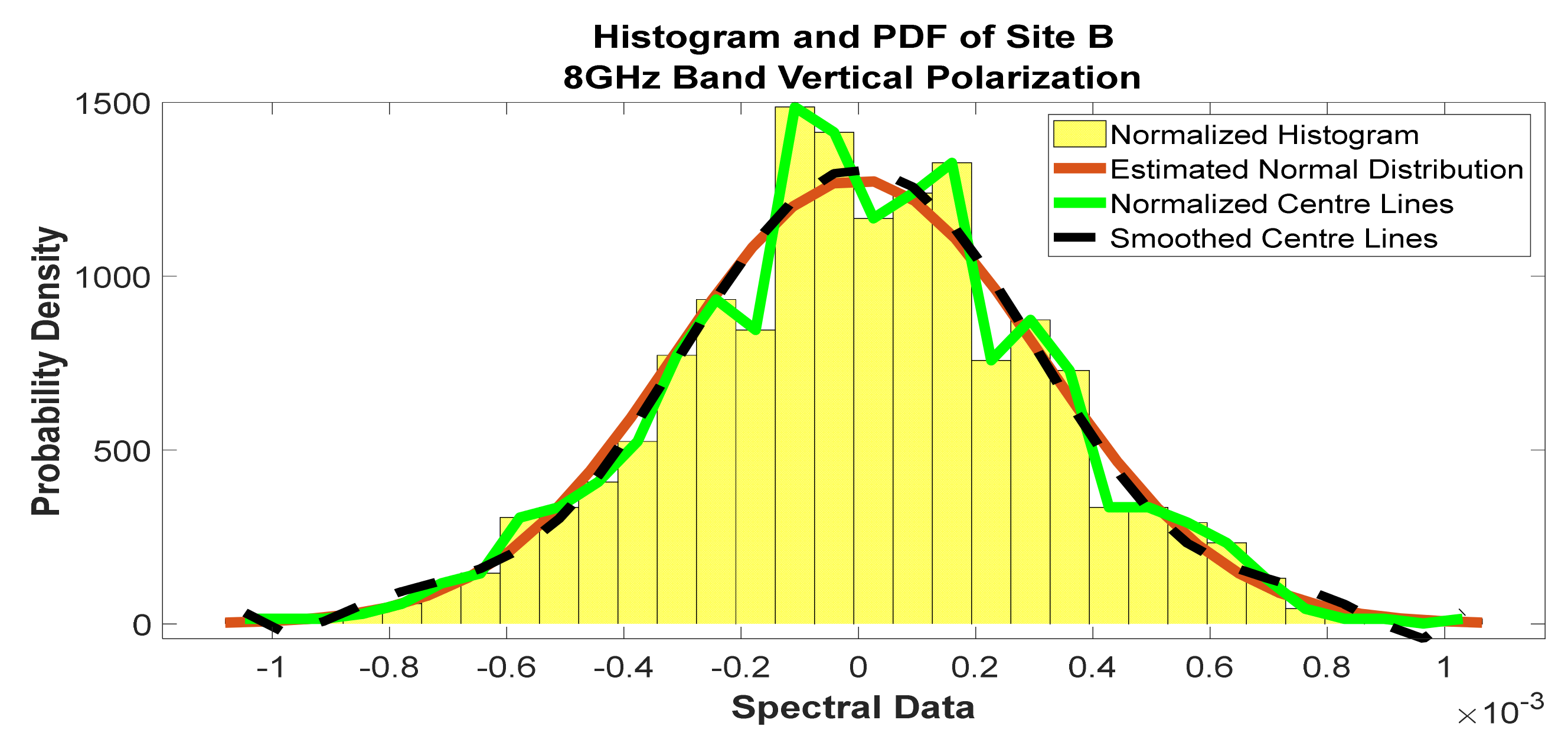
Figure 32.
Histogram and PDF of the frequency scan for site B at 8 GHz vertical polarization.
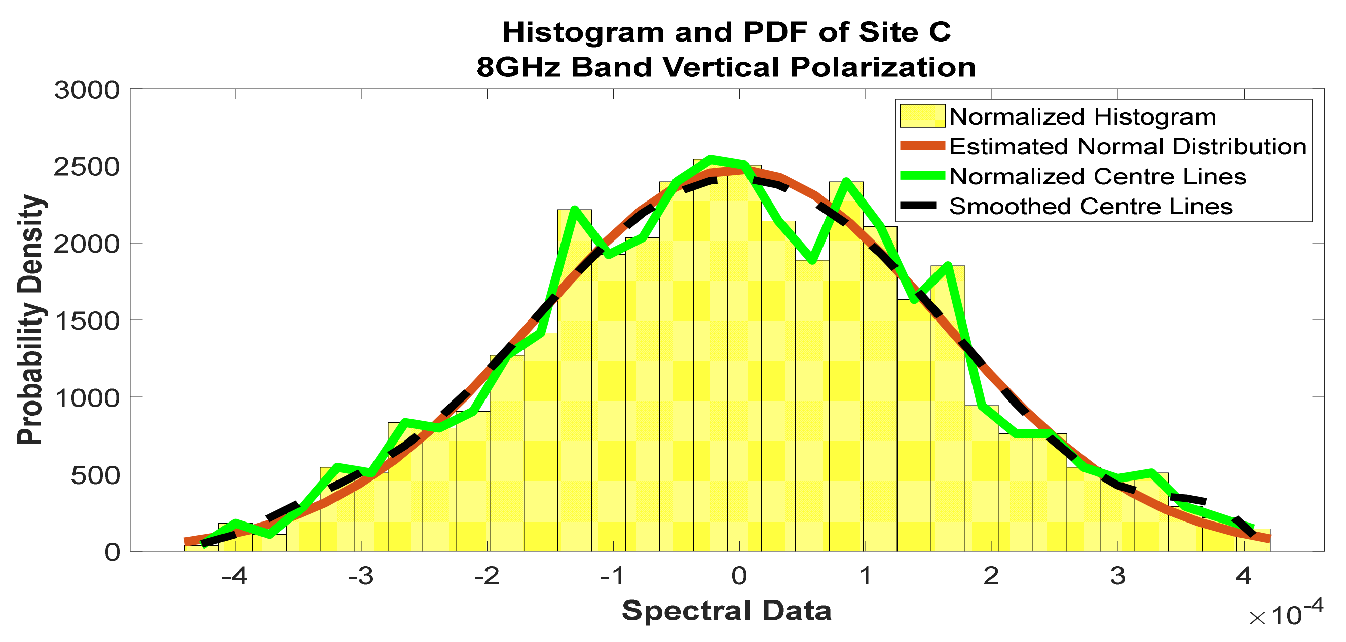
Figure 33.
Histogram and PDF of the frequency scan for site C at 8 GHz vertical polarization.
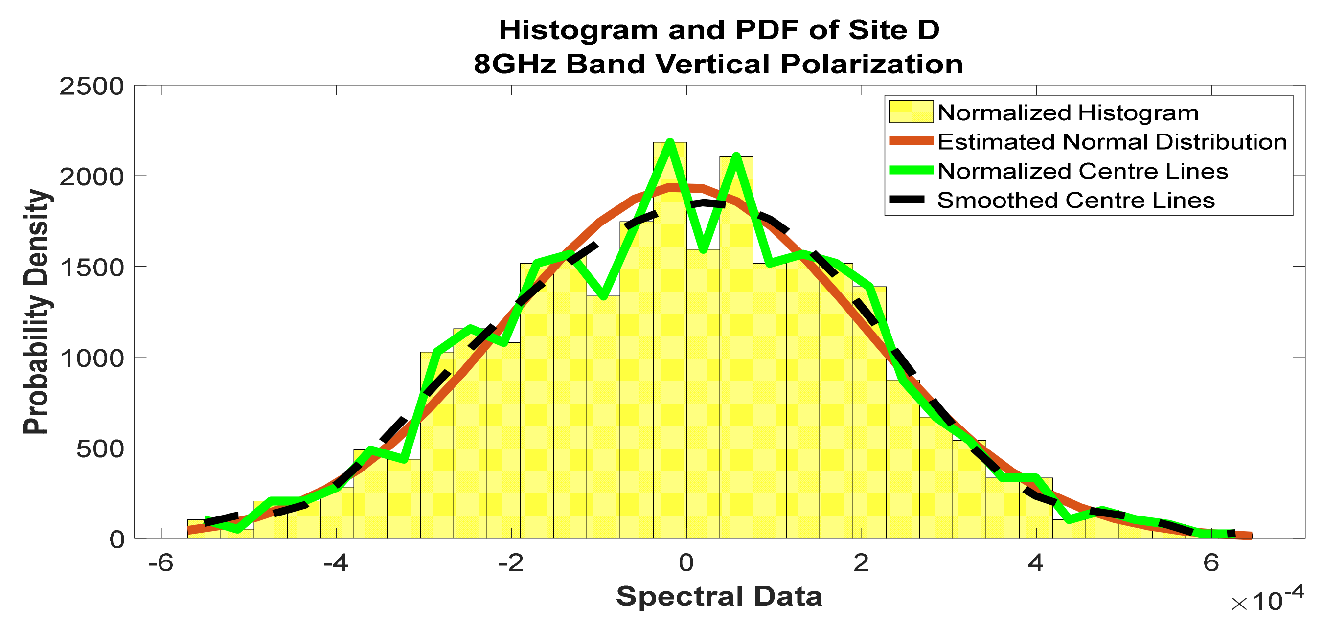
Figure 34.
Histogram and PDF of the frequency scan for site D at 8 GHz vertical polarization.
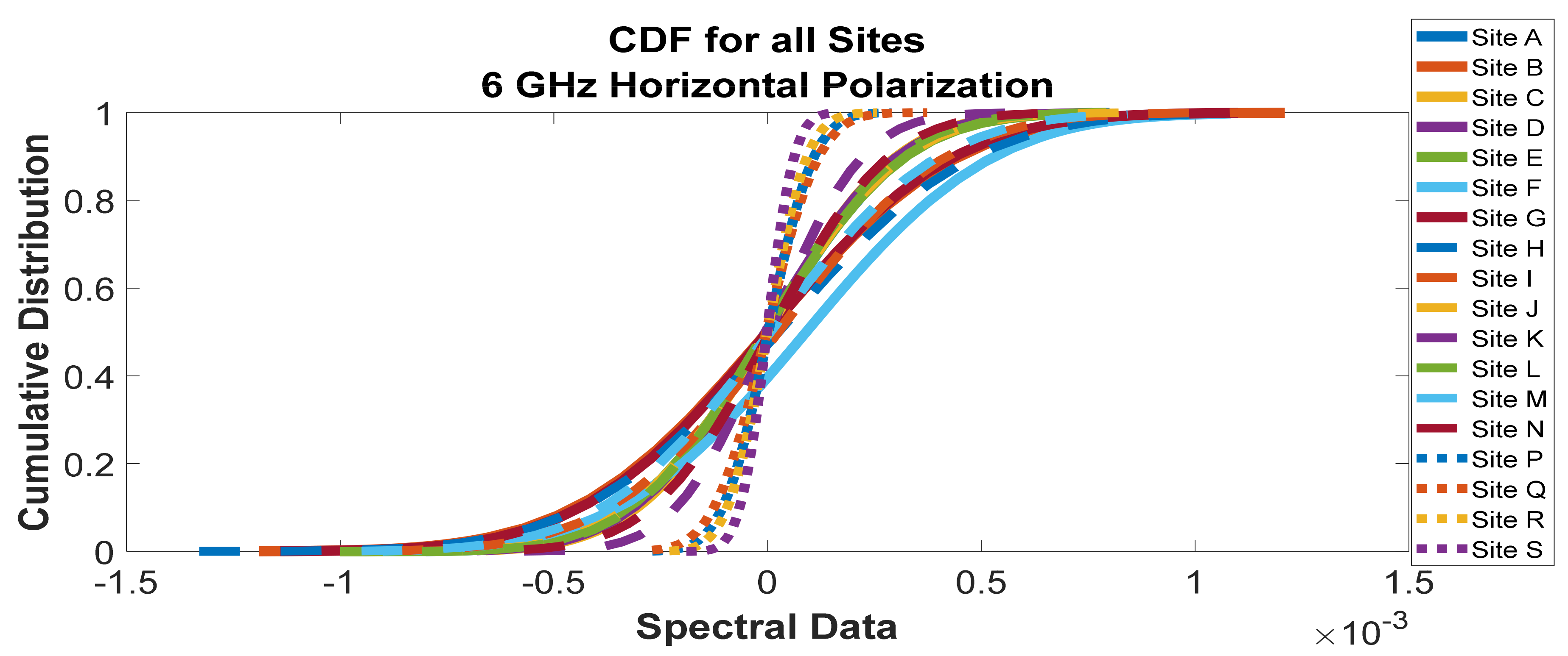
Figure 35.
Cumulative distribution functions of frequency scan for all sites at 6 GHz horizontal polarization.
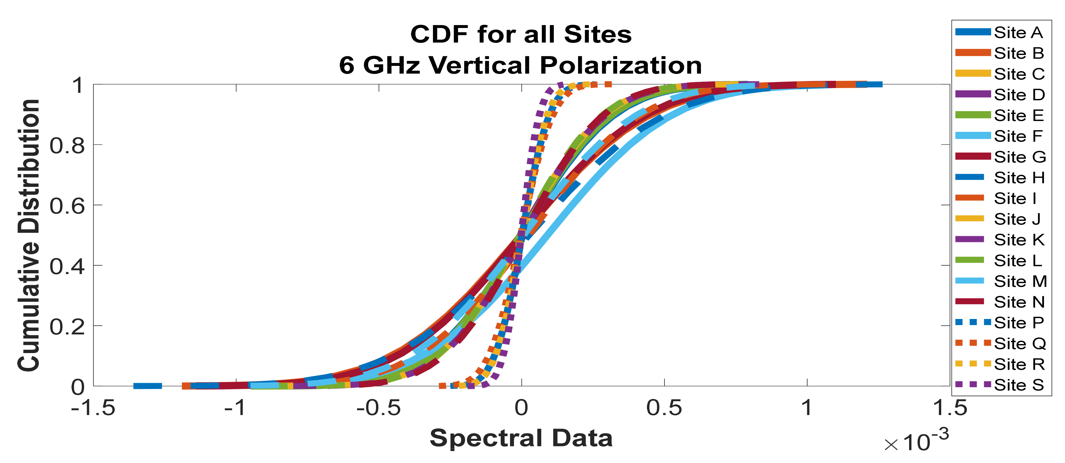
Figure 36.
Cumulative distribution functions of frequency scan for all sites at 6 GHz vertical polarization.
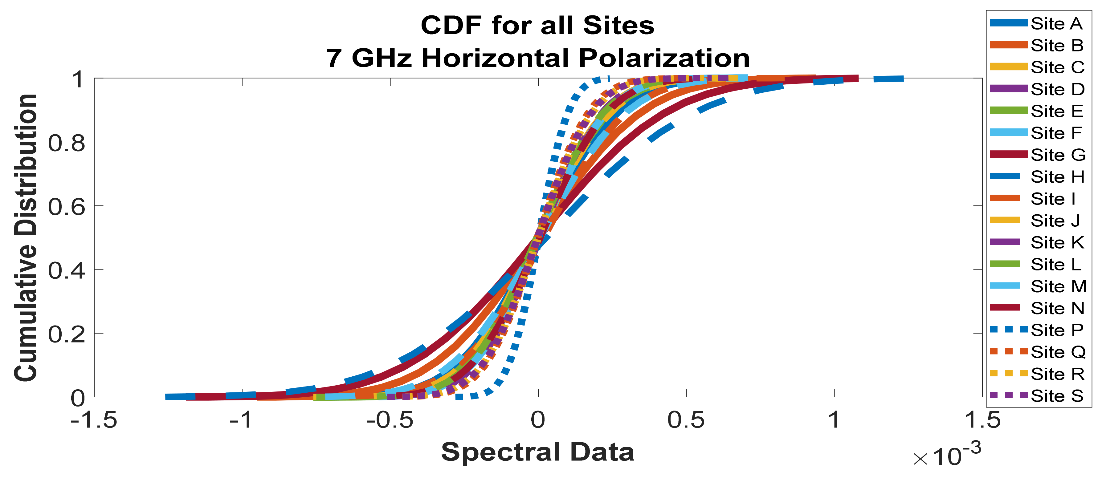
Figure 37.
Cumulative distribution functions of frequency scan for all sites at 7 GHz horizontal polarization.
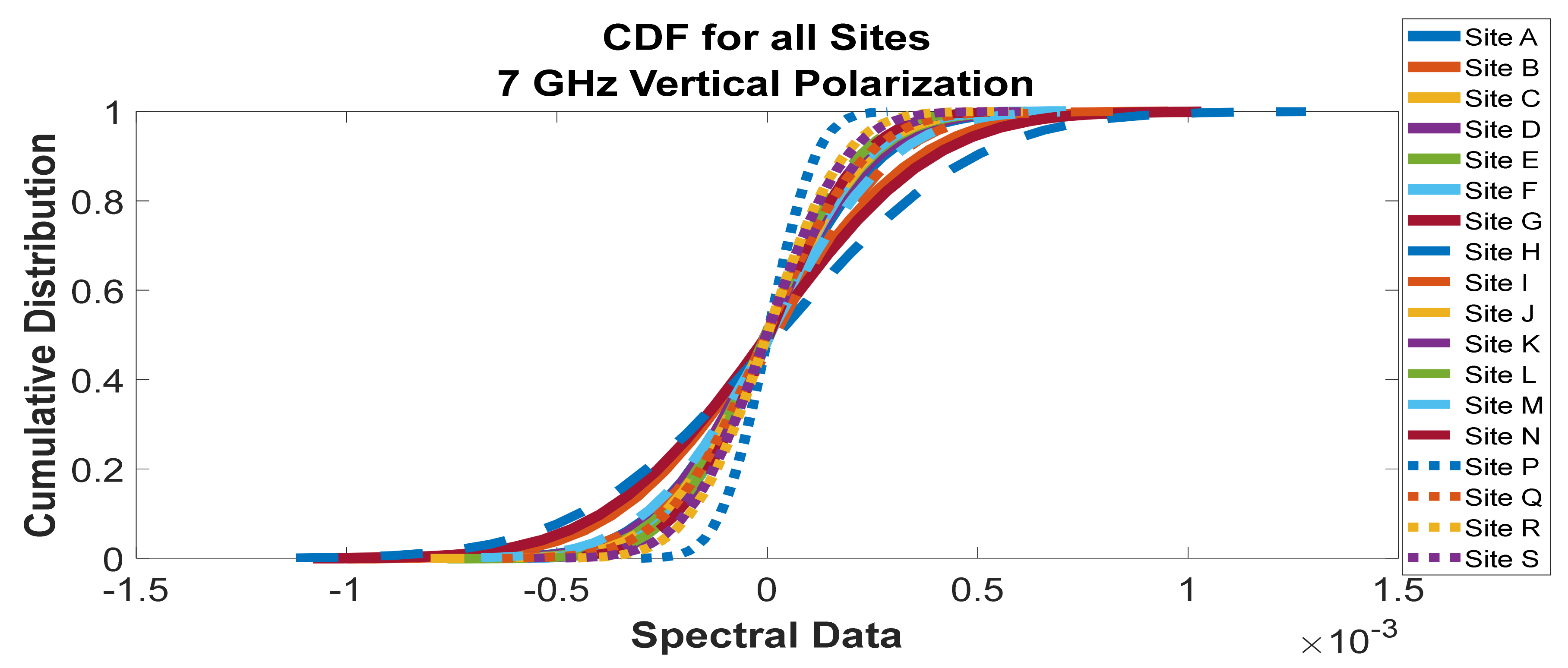
Figure 38.
Cumulative distribution functions of frequency scan for all sites at 7 GHz vertical polarization.
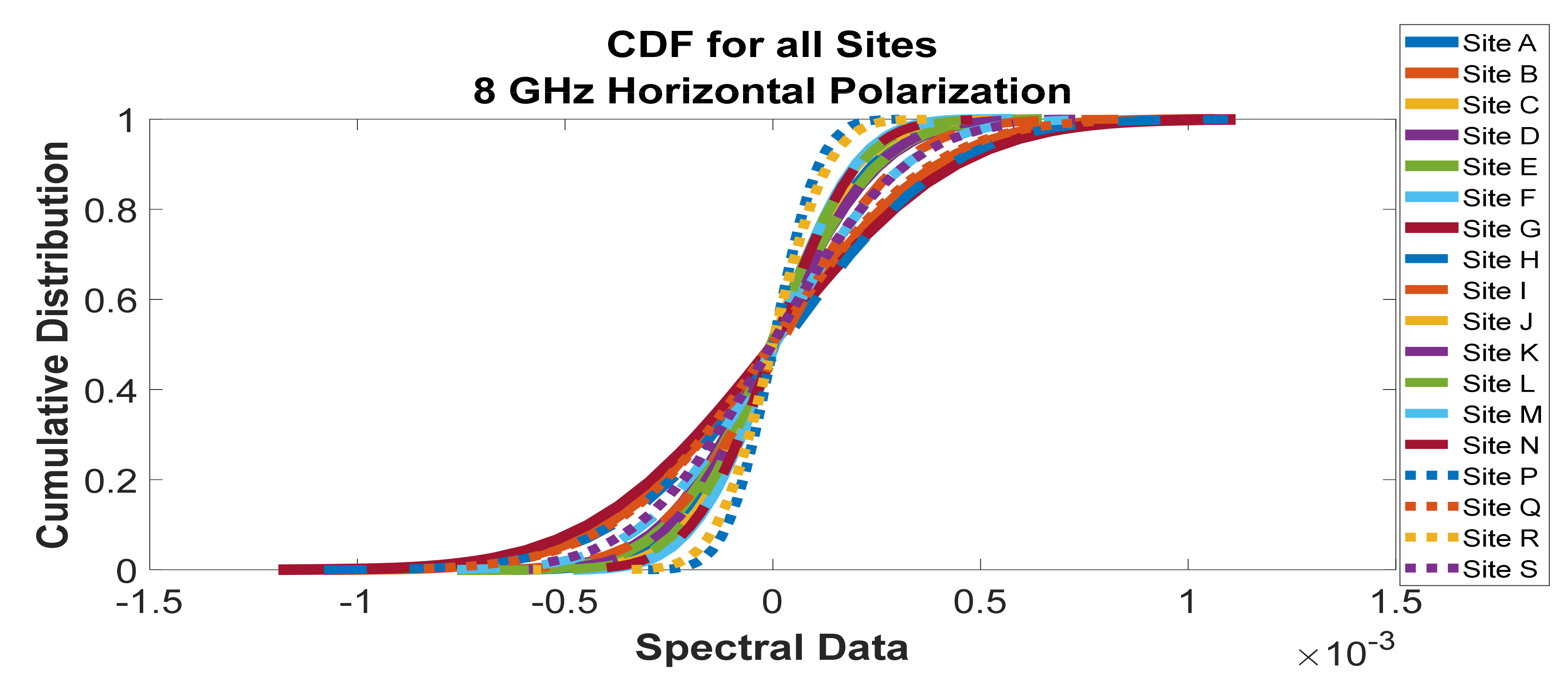
Figure 39.
Cumulative distribution functions of frequency scan for all sites at 8 GHz horizontal polarization.
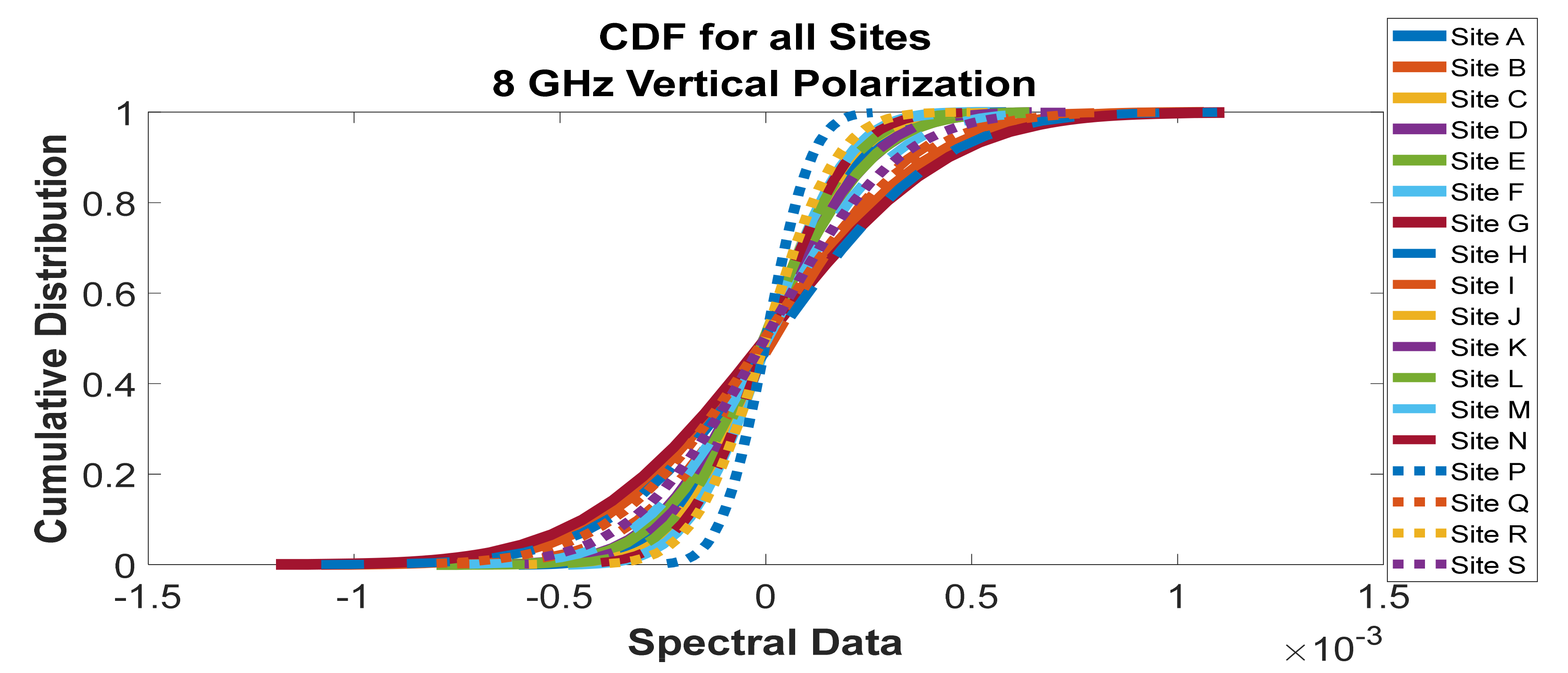
Figure 40.
Cumulative distribution functions of frequency scan for all sites at 8 GHz vertical polarization.
Figure 41.
The 6 GHz horizontal polarization scan for all sites after denoising and applying the algorithm to all sites, including those without the potential to cause interference.
Figure 42.
The 6 GHz vertical polarization scan for all sites after denoising and applying the algorithm to all sites, including those without the potential to cause interference.
Figure 43.
The 7 GHz horizontal polarization scan for all sites after denoising and applying the algorithm to all sites, including those without the potential to cause interference.
Figure 44.
The 7 GHz vertical polarization scan for all sites after denoising and applying the algorithm to all sites, including those without the potential to cause interference.
Figure 45.
The 8 GHz horizontal polarization scan for all sites after denoising and applying the algorithm to all sites, including those without the potential to cause interference.
Figure 46.
The 8 GHz vertical polarization scan for all sites after denoising and applying the algorithm to all sites, including those without the potential to cause interference.
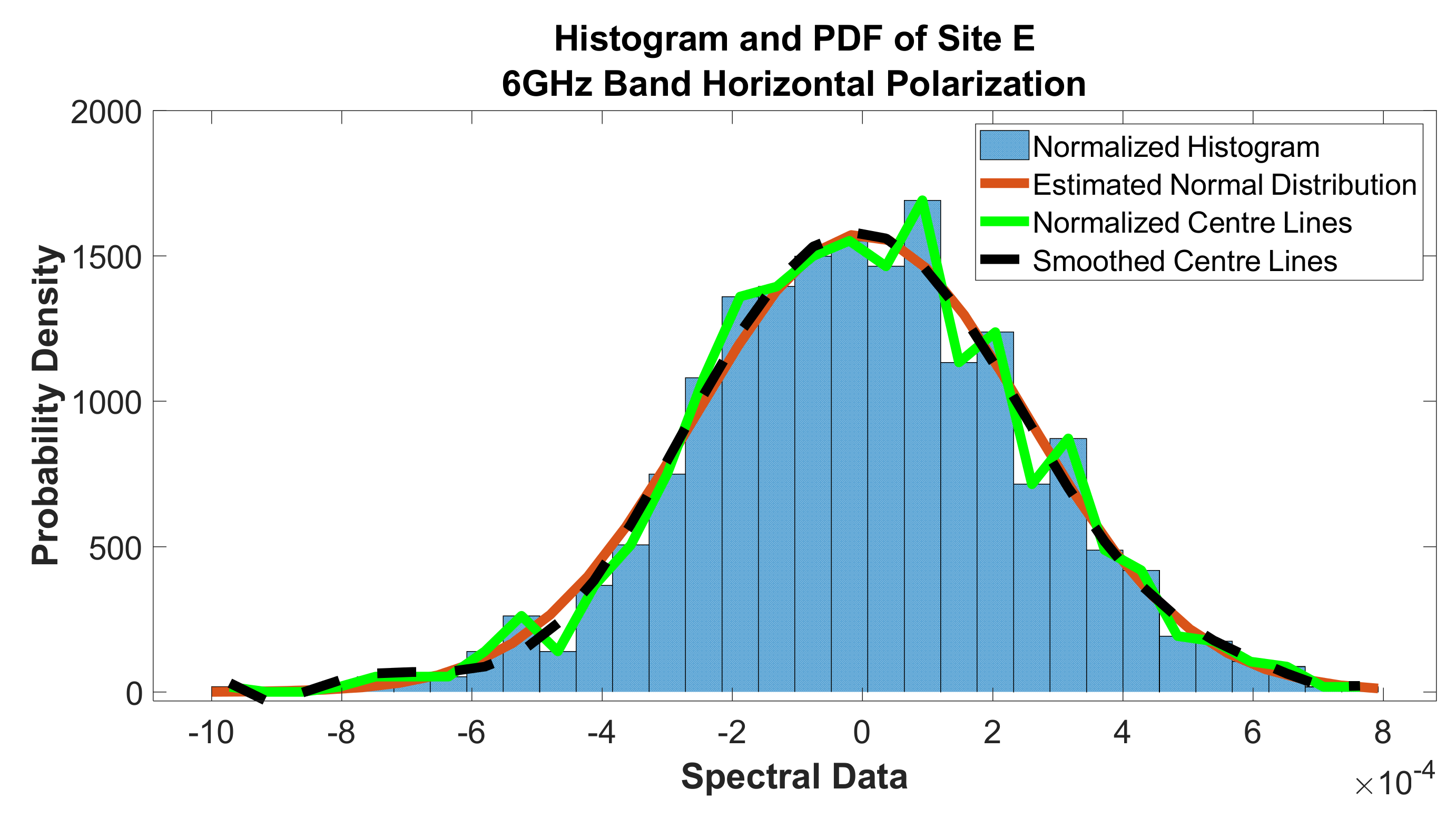
Figure 47.
Histogram and PDF of site E at 6 GHz band horizontal polarization.
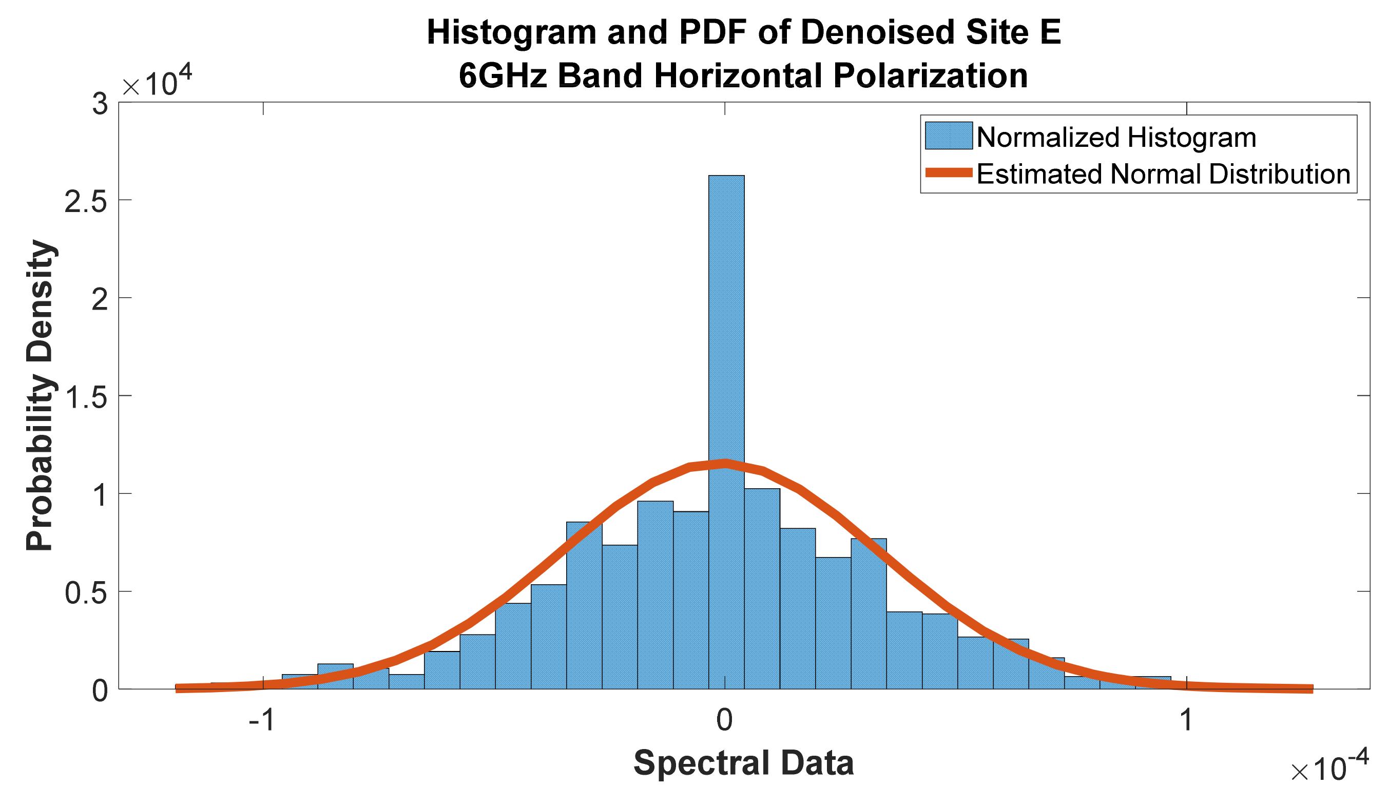
Figure 48.
Histogram and PDF of Denoised Site E at 6 GHz band horizontal polarization.
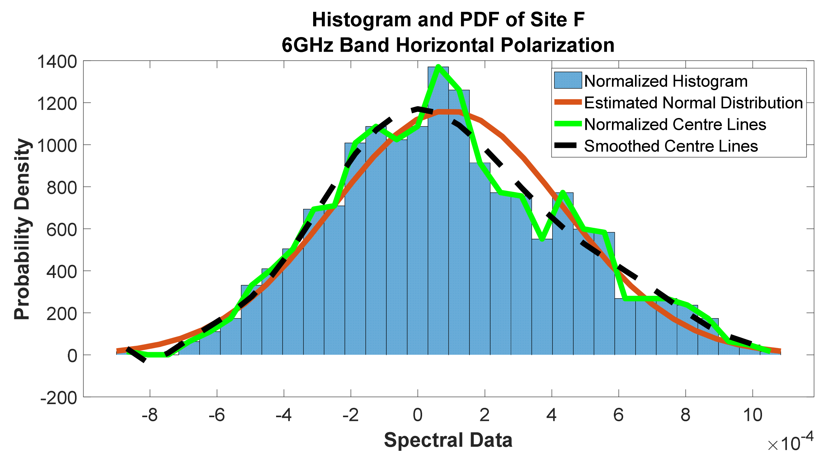
Figure 49.
Histogram and PDF of site F at 6 GHz band horizontal polarization.
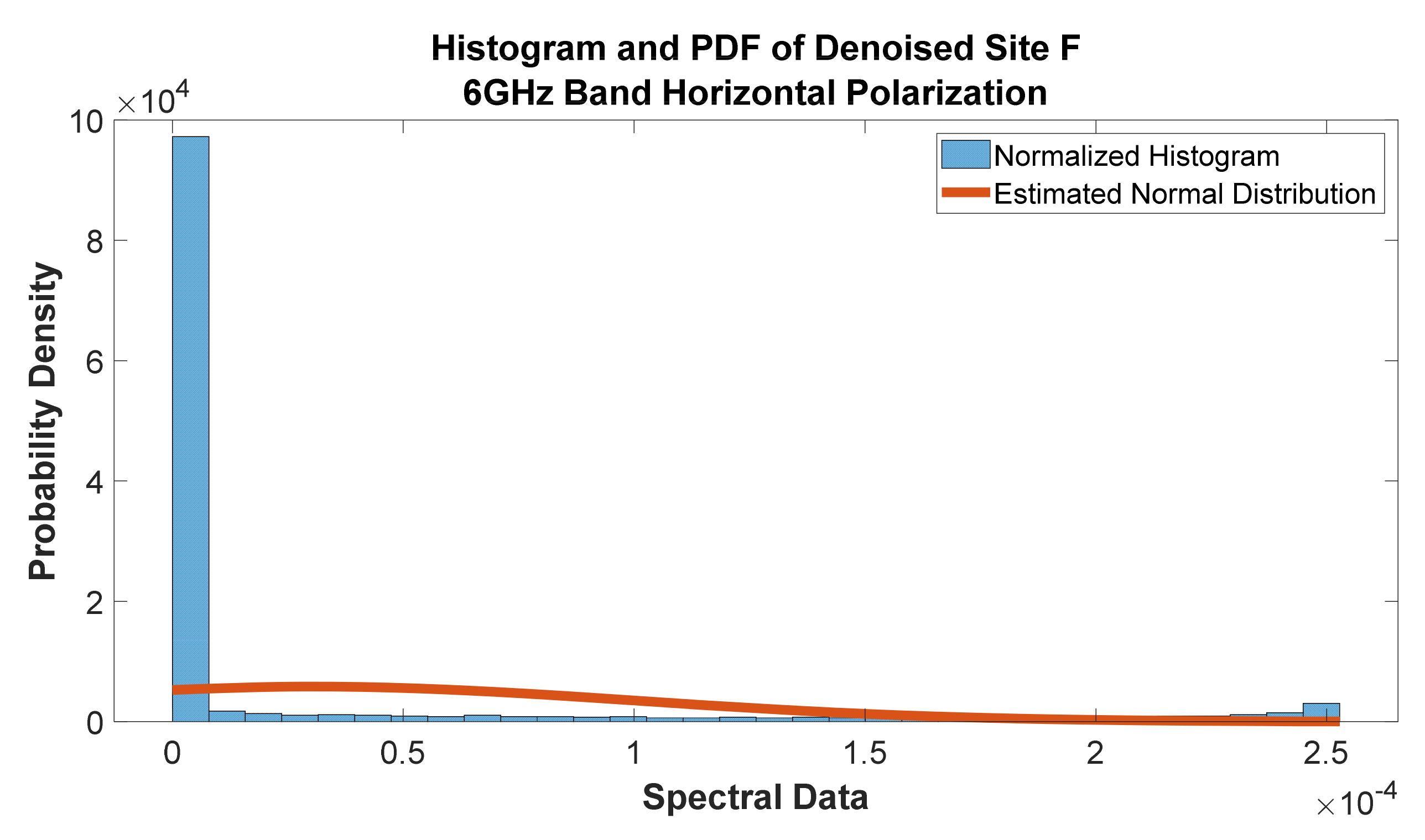
Figure 50.
Histogram and PDF of Denoised Site F at 6 GHz band horizontal polarization.
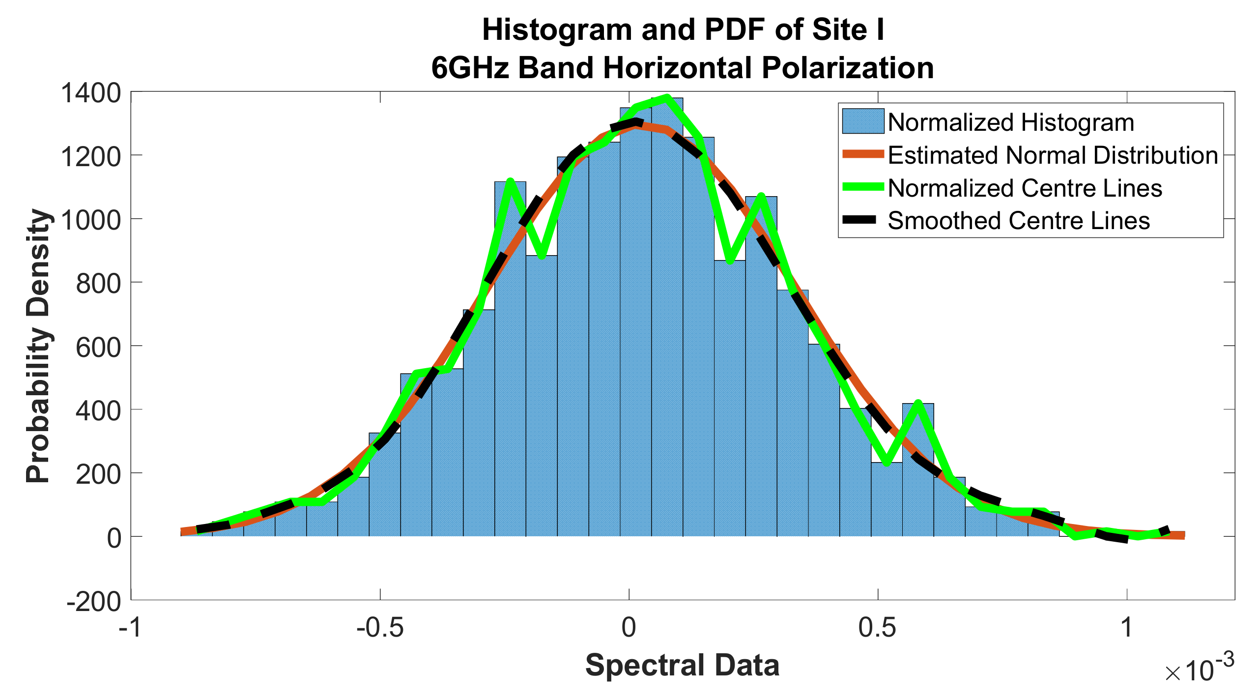
Figure 51.
Histogram and PDF of site I at 6 GHz band horizontal polarization.
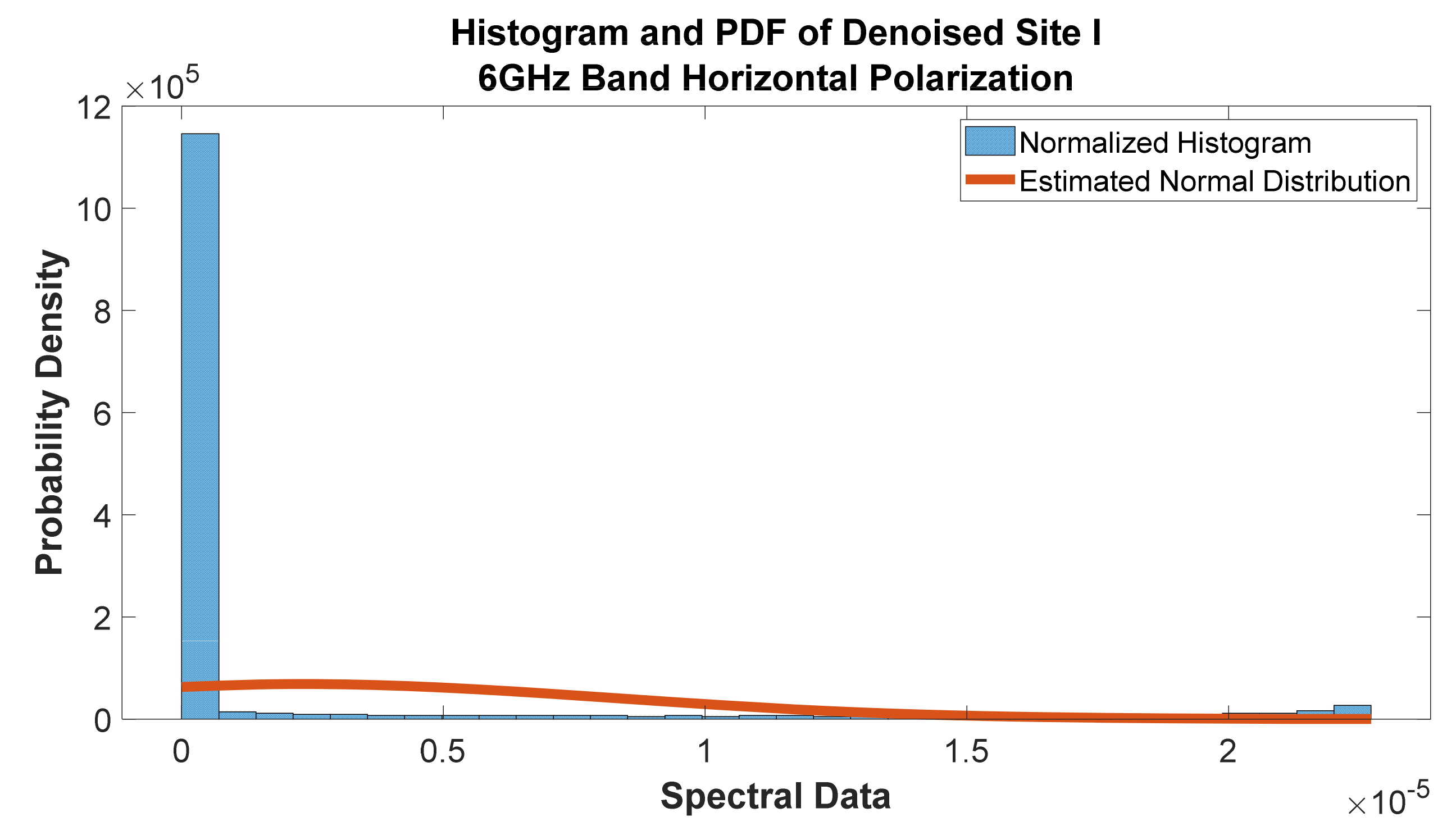
Figure 52.
Histogram and PDF of Denoised Site I at 6 GHz band horizontal polarization.
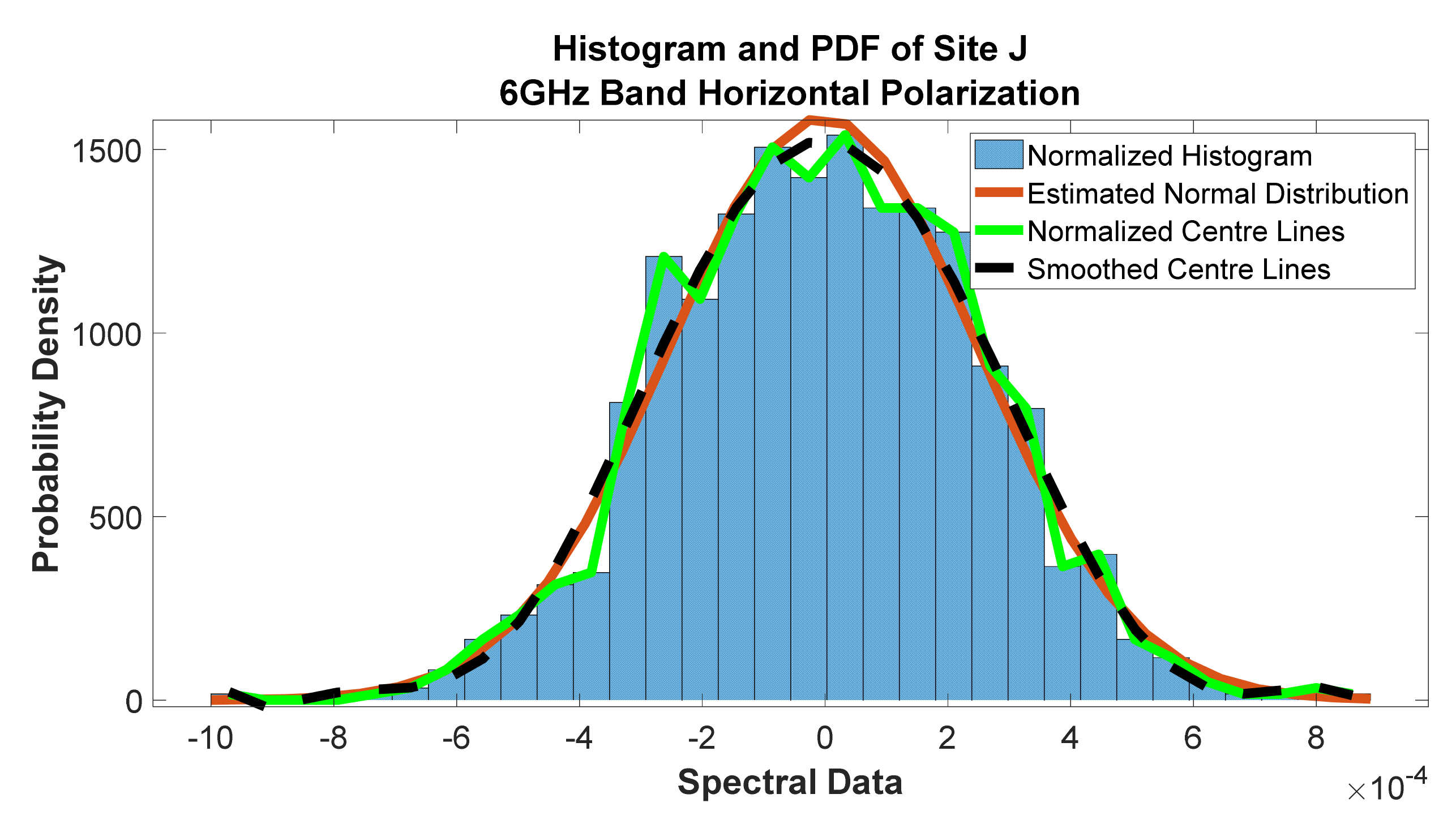
Figure 53.
Histogram and PDF of site J at 6 GHz band horizontal polarization.
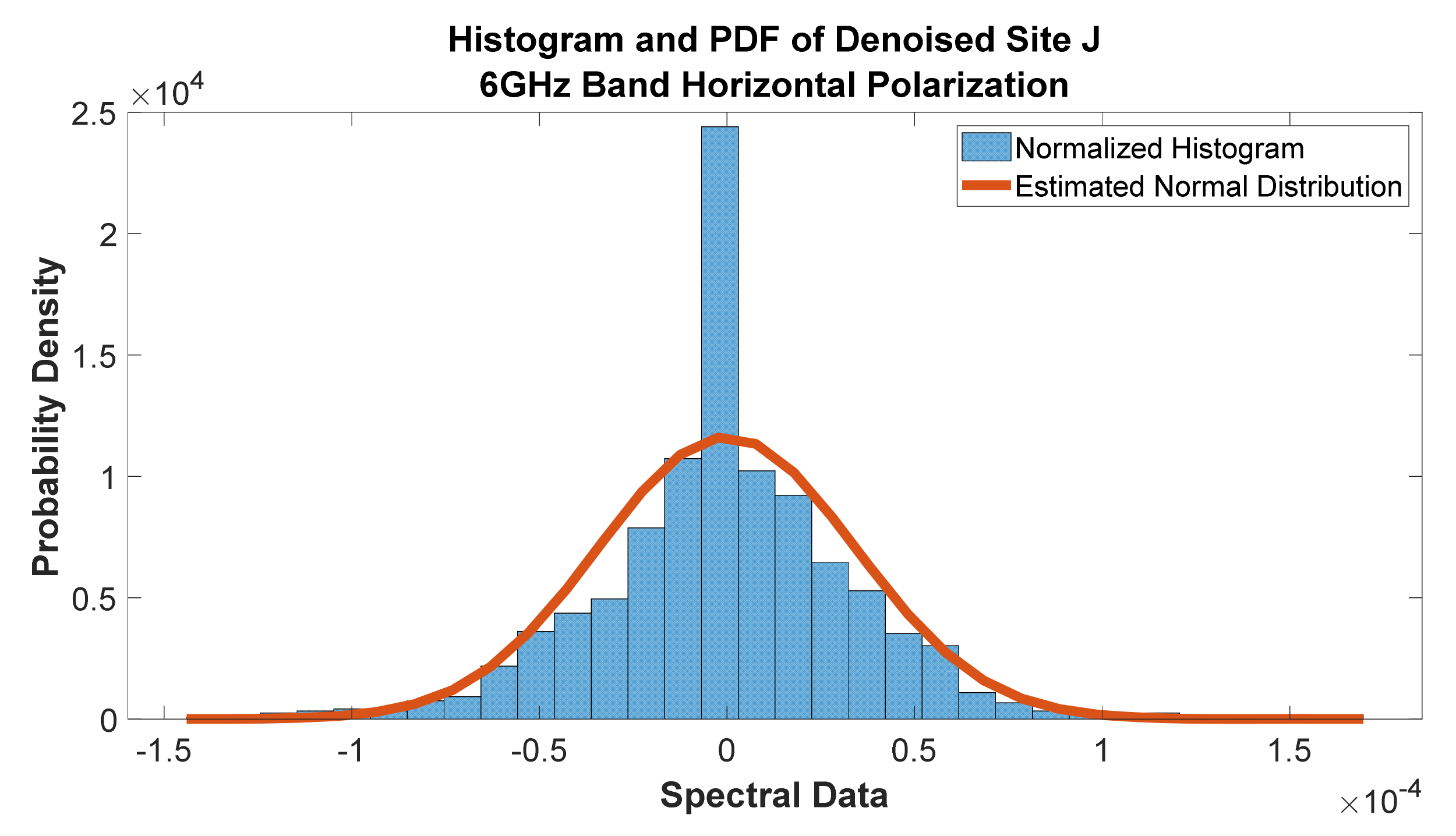
Figure 54.
Histogram and PDF of Denoised Site J at 6 GHz band horizontal polarization.
Table 1.
A comparative analysis of RIS features with other relay systems.
| Features | Reconfigurable Intelligent Surfaces (RIS) | Active, Intelligent Surface-Based Massive MIMO | Backscatter Communication | Amplify and Forward Relay |
|---|
| Hardware architecture | Passive elements | Active elements | Active elements | Active elements |
| Power consumption | Low | High | High | High |
| Environment propagation control | Adjusts the phase shift through intelligent controllers. | - | Reflects received signals from external sources like TV. | - |
| Noise effect | Only reflects the received signal | The use of artificial noise is helpful to the system [40]. | The backscatter signals are weak and with a low signal-to-noise ratio. | Amplifies received signal and receiver noise |
| The unit cost of deployment | Low | High | Low | Low |
Table 2.
Summary of related works, including contributions, key findings and limitations.
| Refs. | Scope and Focus | Contributions | Limitations |
|---|
| [1] | Radio frequency interference measurements. Several measurements and testing equipment were deployed. | Sporadic, continual, and equipment-related signals causing interference were identified during the extensive RFI measurements. | Though grounding systems were installed to mitigate the impact of sporadic emissions, those linked to wind blowing remain. |
| [4] | Radio frequency interference detection and mitigation algorithms. | Several RFI detection and mitigation algorithms by two-dimensional filtering were derived, leveraging spectrogram analysis. | The algorithms were only tested with sinusoidal, chirp, PRN, and OFDM-like signals. The need to test other types of RFI signals with these algorithms remains. |
| [5] | Radio frequency interference detection and mitigation | Compressive statistical sensing (CSS) was introduced to detect and mitigate radio frequency interference. | Further analysis to determine the actual performance of the algorithm under a hardware-based implementation is required. |
| [7] | Radio frequency interference detection on satellite observations. | A factor analysis-based method was proposed for radio frequency interference detection on satellite observations. | RFI detection uncertainties associated with the proposed method remain due to the lack of independent validation datasets. |
| [8] | Radio frequency interference measurement experimentation | A new proposition on using a geostationary satellite with a high gain, steerable antenna to survey the Earth for sources of potential RFI was reported. | Further data analysis is required to determine the relative accuracy of predictions for RFI power flux density. |
| [9] | Systems and methods for determining radio frequency interference | A new technique involves pointing a narrow beam antenna on the satellite at the terrestrial region to determine the presence, frequency, and amplitude of radio frequency interference superimposed on communication. | The systems and methods described appear quite complex and may pose huge design costs. |
| [15] | A review of RFI mitigation techniques in microwave radiometry, including real aperture and aperture synthesis techniques, was covered. | Discussion and assessment of the application of RFI mitigation techniques were presented.
The feasibility of RFI detection and mitigation at one bit and level two is restated. | The findings from the survey would require further experimentation for results validation. |
| [17] | L-Band radio frequency interference environment | Characterization of the L-Band radio frequency interference environment using SMAP radiometer observations | Further analysis of the L-band RFI characteristics based on their temporal and spatial distributions is required. |
| [19] | Radio frequency interference site survey for radio telescopes in Thailand. | The variability of the signal intensity according to the presence of the neighboring population and topography is investigated. | More intensive RFI measurements at some of the sites are required to validate the results. |
| [22] | Transfer function-based calculation method for radio frequency interference. | A transfer function-based calculation method is proposed to estimate RFI problems.
Closed-form equations are analytically derived from Maxwell’s equations and the reciprocity theorem. | Though numeric simulations and real cellphone experiments have been reported, further insights are required to ease the practical implementation of the equations. |
| [23] | Radio frequency interference suppression in NQR experiments | A decision tree pattern recognition model was developed for radio frequency interference suppression in NQR experiments. | Sensitivity is not assessed because the ROC curves do not discriminate the data as a function of the sample mass. |
| [24] | Power control for physical-layer broadcasting using intelligent reflecting surface aided network | A joint design of the transmit beamforming at the BS and the phase shifts of the RIS units. Derivation of the lower bound of the minimum transmits power for the broadcast setting. | Only analytical and simulation results are reported. Experimental implementation remains. |
| [25] | Intelligent Reflecting Surface-Enhanced Wireless Network via Joint Active and Passive Beamforming | Joint optimization of the (active) transmit beamforming at the AP and (passive) reflect beamforming by the phase shifters at the IRS to minimize the total transmit power at the AP under a given set of signal-to-interference-plus-noise ratio (SINR) constraints at the user receivers | Effective self-interference cancellation (SIC), which incurs more energy consumption, would be required to achieve spectrum efficiency |
| [28] | Smart and reconfigurable environment: intelligent reflecting surface aided wireless network | An overview of the promising RIS technology for achieving a smart and reconfigurable environment in future wireless networks. | Practical deployment of the RIS is not covered in work. |
| [30] | Passive beamforming and information transfer via large, intelligent surface | A PBIT-enhanced wireless system, in which a LIS simultaneously enhances the user-BS communication and transmits information to the receiver, is proposed. | The numerical results show that the proposed PBIT system is superior to the preliminaries. However, practical implementation of the LIS-enabled system remains. |
| [43] | Intelligent reflecting surface assisted wireless communication: modeling and channel estimation | A minimum means squared error-based channel estimation protocol for the design and analysis of IRS-assisted systems was proposed. | Experimentally validated channel models that provide pathloss and fast fading parameters for IRS-assisted links under different implementations are required. |
Table 3.
Frequency usage plan for the three different frequency bands tested.
| Frequency Band | Start Frequency | Stop Frequency | Frequency Span |
|---|
| 6 GHz | 5.9 GHz | 6.5 GHz | 600 MHz |
| 7 GHz | 7.4 GHz | 7.8 GHz | 400 MHz |
| 8 GHz | 7.7 GHz | 8.3 GHz | 600 MHz |
Table 4.
Step-by-step procedure for measured data processing and analysis.
| S/N. | Procedure | Specific Task |
|---|
| 1. | Replicating the spectrum analyzer frequency scans | - (a)
Specify the sample rate frequency; - (b)
Specify the offset frequency; - (c)
Specify the number of averages; - (d)
Determine the type of noise at the site; - (e)
Specify the power of the noise; - (f)
Generate signals at specified frequencies, as shown in the scans.; - (g)
For multiple scan results on a graph, specify the number of input ports.
|
| 2. | Statistical characteristics | - (a)
Generate the histogram of the site scan data; - (b)
Observe the distribution of the generated histogram and then generate an approximate distribution for the data; - (c)
For the site data, obtain the mean, median, standard deviation, variance, interquartile range, skewness, and Kurtosis; - (d)
For the estimated distribution, obtain the negative loglikelihood, lower and upper confidence intervals for the standard deviation; - (e)
Generate a line graph connecting the centers of the histograms; - (f)
Generate a smooth line approximating the generated line graph using 9th order polynomial.
|
| 3. | Error Analysis for each of the approximated distributions and generated smoothed line | - (a)
Obtain the following statistical parameters between the actual site data and each of the estimated distribution and generated smoothed lines:
Mean Absolute Error (MAE); Root Mean Square Error (RMSE); Mean Absolute Percentage Error (MAPE); Mean Squared Error (MSE); Relative Absolute Error (RAE).
- (b)
Generate the probability distribution function and the cumulative distribution functions.
|
| 4. | Signal denoising process | The step-by-step process of the signal denoising is described as follows:- (1)
Using a suitable window, obtain the short-time Fourier transform (STFT) of the noisy signal; - (2)
Square the absolute values of the results obtained in (1); - (3)
Sort the results obtained in (2) in descending order; - (4)
Obtain the cumulative sum of the results obtained in (3); - (5)
Identify the values of (4) that have more than 30% of the power. Set this as the threshold value; - (6)
Find the values of (2) that are greater than the threshold value; - (7)
The next step is the denoising of the signal through multiplying (1) by (6); - (8)
Recover the signal without noise through inverse short-time Fourier transform (ISTFT).
|
Table 5.
The desired frequencies for the 18 channels at 6 GHz: Available (A); Not Available (NA).
| Freq. | A | B | C | D | E | F | G | H | I | J | K | L | M | N | P | Q | R | S |
|---|
| 5.945 | A | A | A | A | A | NA | NA | NA | A | NA | NA | A | A | A | A | A | A | A |
| 5.975 | A | A | A | A | A | NA | NA | NA | A | A | NA | A | NA | A | A | A | A | A |
| 6.005 | A | A | A | A | A | NA | NA | NA | A | NA | A | A | A | A | A | A | A | A |
| 6.034 | A | NA | A | NA | A | NA | NA | NA | A | NA | NA | A | A | A | NA | NA | A | A |
| 6.093 | A | A | A | NA | A | NA | NA | NA | A | A | NA | A | A | A | A | A | A | A |
| 6.153 | A | A | A | A | A | NA | NA | NA | A | A | A | A | A | A | NA | NA | A | NA |
Table 6.
Error analysis for the estimated normal distribution (Y) and the estimated fitness curve (F), where the first five columns describe the error in the PDF and the last five columns describe the errors in the fitness curve for the 6 GHz horizontal polarization.
| Sites | MAE_Y | RMSE_Y | MAPE_Y | RAE_Y | | MAE_F | RMSE_F | MAPE_F | RAE_F | |
|---|
| A | 81.14 | 115.97 | 0.2716 | 0.1367 | 1.3450 | 85.64 | 111.81 | 0.3255 | 0.1318 | 1.2501 |
| B | 57.19 | 79.04 | 0.3929 | 0.1348 | 0.6246 | 61.30 | 78.57 | 1.5153 | 0.1340 | 0.6174 |
| C | 73.02 | 92.22 | 0.1887 | 0.0961 | 0.8505 | 60.48 | 77.62 | 0.1590 | 0.0809 | 0.6025 |
| D | 80.60 | 125.03 | 0.2365 | 0.1387 | 1.5633 | 75.92 | 107.03 | 0.2787 | 0.1187 | 1.1455 |
| E | 62.79 | 90.56 | 0.3388 | 0.1137 | 0.8201 | 61.05 | 86.49 | 1.2433 | 0.1086 | 0.7480 |
| F | 87.88 | 116.69 | 2.6438 | 0.1806 | 1.3612 | 65.16 | 86.52 | 1.6073 | 0.1339 | 0.7486 |
| G | 51.97 | 78.61 | 1.0338 | 0.1295 | 0.6177 | 46.00 | 59.56 | 2.4757 | 0.0981 | 0.3547 |
| H | 44.44 | 62.00 | 0.5683 | 0.1076 | 0.3844 | 41.97 | 59.37 | 0.4917 | 0.1031 | 0.3525 |
| I | 55.38 | 85.19 | 0.8604 | 0.1252 | 0.7257 | 55.44 | 82.70 | 1.6589 | 0.1215 | 0.6840 |
| J | 56.83 | 91.09 | 0.5348 | 0.1180 | 0.8296 | 50.58 | 76.64 | 1.4309 | 0.0993 | 0.5874 |
| K | 101.26 | 144.58 | 1.2996 | 0.1212 | 2.0902 | 87.15 | 134.37 | 0.9198 | 0.1126 | 1.8055 |
| L | 61.00 | 86.01 | 0.5199 | 0.1020 | 0.7398 | 56.78 | 80.17 | 1.4000 | 0.0951 | 0.6427 |
| M | 72.58 | 99.47 | 1.2024 | 0.1390 | 0.9892 | 61.46 | 89.07 | 1.7965 | 0.1245 | 0.7934 |
| N | 111.13 | 145.61 | 1.6398 | 0.1422 | 2.1200 | 100.35 | 135.57 | 2.3125 | 0.1324 | 1.8378 |
| P | 199.62 | 280.51 | 3.7499 | 0.1131 | 7.8677 | 180.88 | 248.04 | 3.5667 | 0.1000 | 6.1521 |
| Q | 146.20 | 201.68 | 1.6824 | 0.0941 | 4.0673 | 127.28 | 174.96 | 1.9093 | 0.0816 | 3.0610 |
| R | 253.38 | 410.28 | 0.9086 | 0.1446 | 16.8327 | 252.58 | 381.94 | 0.7003 | 0.1346 | 14.5876 |
| S | 372.28 | 568.43 | 13.6276 | 0.1373 | 32.3082 | 331.23 | 539.07 | 17.4459 | 0.1302 | 29.0599 |
Table 7.
Error analysis for the estimated normal distribution (Y) and the estimated fitness curve (F), where the first five columns describe the error in the PDF and the last five columns describe the errors in the fitness curve for the 6 GHz vertical polarization.
| Sites | MAE_Y | RMSE_Y | MAPE_Y | RAE_Y | | MAE_F | RMSE_F | MAPE_F | RAE_F | |
|---|
| A | 80.63 | 98.93 | 1.6353 | 0.1190 | 0.9784 | 69.27 | 91.10 | 1.6878 | 0.1096 | 0.8300 |
| B | 58.34 | 80.19 | 0.4142 | 0.1373 | 0.6431 | 62.16 | 79.74 | 1.5288 | 0.1365 | 0.6359 |
| C | 81.31 | 115.62 | 0.1963 | 0.1221 | 1.3369 | 68.73 | 105.55 | 0.1750 | 0.1114 | 1.1140 |
| D | 76.52 | 105.09 | 0.1930 | 0.1148 | 1.1045 | 66.75 | 83.65 | 0.1789 | 0.0913 | 0.6996 |
| E | 80.32 | 123.98 | 1.0729 | 0.1500 | 1.5372 | 79.08 | 120.37 | 3.9053 | 0.1457 | 1.4489 |
| F | 87.82 | 116.67 | 2.6438 | 0.1806 | 1.3612 | 65.16 | 86.52 | 1.6073 | 0.1339 | 0.7486 |
| G | 51.91 | 78.59 | 1.0338 | 0.1295 | 0.6177 | 46.00 | 59.56 | 2.4757 | 0.0981 | 0.3547 |
| H | 44.46 | 66.01 | 0.9776 | 0.1222 | 0.4358 | 45.74 | 64.17 | 2.4783 | 0.1188 | 0.4118 |
| I | 55.32 | 85.19 | 0.8604 | 0.1252 | 0.7257 | 55.44 | 82.70 | 1.6589 | 0.1215 | 0.6840 |
| J | 58.53 | 99.68 | 0.6650 | 0.1168 | 0.9936 | 48.73 | 81.89 | 1.6793 | 0.0959 | 0.6706 |
| K | 58.61 | 97.20 | 0.4869 | 0.1106 | 0.9447 | 57.23 | 85.82 | 1.3762 | 0.0977 | 0.7365 |
| L | 62.25 | 89.44 | 0.5839 | 0.0996 | 0.7999 | 54.84 | 85.03 | 1.3270 | 0.0947 | 0.7229 |
| M | 68.71 | 91.35 | 0.2786 | 0.1297 | 0.8345 | 57.31 | 81.01 | 0.2522 | 0.1150 | 0.6562 |
| N | 103.15 | 139.66 | 0.2687 | 0.1373 | 1.9505 | 98.50 | 129.72 | 0.2840 | 0.1276 | 1.6828 |
| P | 247.14 | 313.64 | 8.2762 | 0.1143 | 9.8368 | 212.26 | 288.36 | 6.4423 | 0.1050 | 8.3149 |
| Q | 168.73 | 240.67 | 1.8458 | 0.1038 | 5.7923 | 165.49 | 232.12 | 3.5493 | 0.1001 | 5.3881 |
| R | 266.11 | 395.94 | 3.4193 | 0.1353 | 15.6767 | 252.96 | 361.40 | 5.1626 | 0.1235 | 13.0610 |
| S | 372.16 | 568.40 | 13.6276 | 0.1373 | 32.3082 | 331.23 | 539.07 | 17.4459 | 0.1302 | 29.0599 |
Table 8.
Error analysis for the estimated normal distribution (Y) and the estimated fitness curve (F), where the first five columns describe the error in the PDF and the last five columns describe the errors in the fitness curve for the 7 GHz horizontal polarization.
| Sites | MAE_Y | RMSE_Y | MAPE_Y | RAE_Y | | MAE_F | RMSE_F | MAPE_F | RAE_F | |
|---|
| A | 88.86 | 123.88 | 1.6733 | 0.1273 | 1.5343 | 84.91 | 114.43 | 1.3897 | 0.1176 | 1.3094 |
| B | 63.50 | 93.42 | 0.5082 | 0.1263 | 0.8728 | 64.23 | 90.55 | 1.9711 | 0.1224 | 0.8199 |
| C | 139.01 | 163.20 | 0.2052 | 0.1301 | 2.6635 | 121.88 | 151.59 | 0.1871 | 0.1208 | 2.2981 |
| D | 121.05 | 194.92 | 0.2324 | 0.1704 | 3.7995 | 119.11 | 179.78 | 0.3105 | 0.1572 | 3.2320 |
| E | 83.62 | 129.86 | 0.3822 | 0.1245 | 1.6864 | 80.01 | 124.56 | 1.3817 | 0.1194 | 1.5516 |
| F | 88.76 | 126.17 | 2.1202 | 0.1125 | 1.5918 | 83.92 | 115.31 | 2.7276 | 0.1029 | 1.3297 |
| G | 53.72 | 73.85 | 0.2935 | 0.1230 | 0.5454 | 42.75 | 59.48 | 0.3441 | 0.0991 | 0.3538 |
| H | 65.97 | 91.76 | 0.6539 | 0.1761 | 0.8420 | 59.84 | 85.33 | 0.8471 | 0.1638 | 0.7281 |
| I | 69.78 | 108.30 | 0.6132 | 0.1164 | 1.1729 | 68.74 | 104.69 | 1.2885 | 0.1125 | 1.0960 |
| J | 77.78 | 124.09 | 1.3754 | 0.1247 | 1.5399 | 68.80 | 109.20 | 1.2062 | 0.1097 | 1.1924 |
| K | 96.09 | 145.19 | 0.3791 | 0.1204 | 2.1079 | 90.72 | 136.53 | 0.3677 | 0.1132 | 1.8642 |
| L | 85.00 | 131.92 | 0.2614 | 0.1168 | 1.7402 | 77.06 | 125.75 | 0.9510 | 0.1113 | 1.5814 |
| M | 87.34 | 120.57 | 0.2474 | 0.1293 | 1.4536 | 74.72 | 105.86 | 0.1277 | 0.1136 | 1.1206 |
| N | 154.43 | 225.09 | 0.7704 | 0.1117 | 1.7681 | 84.69 | 113.54 | 0.6018 | 0.0954 | 1.2892 |
| P | 201.75 | 277.06 | 2.1308 | 0.1061 | 7.6762 | 187.23 | 253.44 | 5.1209 | 0.0970 | 6.4231 |
| Q | 166.47 | 225.80 | 0.3395 | 0.1480 | 5.0985 | 118.88 | 148.11 | 0.3891 | 0.0971 | 2.1937 |
| R | 128.10 | 207.16 | 1.0163 | 0.1511 | 4.2915 | 127.68 | 184.76 | 8.5567 | 0.1347 | 3.4138 |
| S | 142.50 | 207.85 | 0.3534 | 0.1478 | 4.3201 | 94.50 | 123.70 | 0.5539 | 0.0880 | 1.5303 |
Table 9.
Error analysis for the estimated normal distribution (Y) and the estimated fitness curve (F), where the first five columns describe the error in the PDF and the last five columns describe the errors in the fitness curve for the 7 GHz vertical polarization.
| Sites | MAE_Y | RMSE_Y | MAPE_Y | RAE_Y | | MAE_F | RMSE_F | MAPE_F | RAE_F | |
|---|
| A | 108.18 | 142.39 | 1.5030 | 0.1420 | 2.0274 | 95.00 | 136.67 | 1.1399 | 0.1363 | 1.8679 |
| B | 61.38 | 94.26 | 0.6658 | 0.1304 | 0.8884 | 61.13 | 91.73 | 2.3281 | 0.1269 | 0.8414 |
| C | 141.95 | 185.35 | 0.2037 | 0.1556 | 3.4356 | 114.28 | 167.03 | 0.1647 | 0.1402 | 2.7898 |
| D | 105.99 | 153.82 | 0.1974 | 0.1454 | 2.3661 | 97.77 | 138.78 | 0.1419 | 0.1312 | 1.9260 |
| E | 83.62 | 129.86 | 0.3822 | 0.1245 | 1.6864 | 80.01 | 124.56 | 1.3817 | 0.1194 | 1.5516 |
| F | 109.64 | 163.02 | 2.3367 | 0.1476 | 2.6574 | 102.76 | 154.54 | 1.8779 | 0.1399 | 2.3883 |
| G | 51.63 | 74.25 | 1.7267 | 0.1124 | 0.5513 | 42.60 | 59.40 | 2.4694 | 0.0899 | 0.3528 |
| H | 57.21 | 83.98 | 0.4309 | 0.1455 | 0.7053 | 53.87 | 77.41 | 0.7717 | 0.1341 | 0.5993 |
| I | 68.41 | 107.53 | 0.6170 | 0.1156 | 1.1562 | 67.35 | 103.87 | 1.3269 | 0.1117 | 1.0789 |
| J | 90.03 | 130.83 | 1.2474 | 0.1292 | 1.7116 | 82.25 | 112.75 | 4.0385 | 0.1114 | 1.2712 |
| K | 77.79 | 101.39 | 0.7099 | 0.0870 | 1.0279 | 62.45 | 88.98 | 1.3740 | 0.0764 | 0.7918 |
| L | 71.61 | 108.77 | 0.5949 | 0.0933 | 1.1830 | 61.04 | 100.15 | 1.6584 | 0.0859 | 1.0031 |
| M | 108.72 | 139.61 | 2.3822 | 0.1479 | 1.9490 | 95.48 | 129.26 | 1.9073 | 0.1370 | 1.6708 |
| N | 159.36 | 207.55 | 0.2529 | 0.1586 | 4.3076 | 144.93 | 193.89 | 0.2773 | 0.1482 | 3.7595 |
| P | 218.98 | 294.38 | 1.8206 | 0.1229 | 8.6661 | 181.85 | 248.85 | 2.0382 | 0.1039 | 6.1929 |
| Q | 202.87 | 278.79 | 0.7323 | 0.2286 | 7.7722 | 136.76 | 175.85 | 3.3330 | 0.1442 | 3.0923 |
| R | 125.07 | 198.27 | 1.8680 | 0.1388 | 3.9312 | 113.09 | 140.29 | 8.6216 | 0.0982 | 1.9681 |
| S | 115.87 | 177.36 | 0.3512 | 0.1287 | 3.1458 | 95.18 | 122.80 | 1.1084 | 0.0891 | 1.5081 |
Table 10.
Error analysis for the estimated normal distribution (Y) and the estimated fitness curve (F), where the first five columns describe the error in the PDF and the last five columns describe the errors in the fitness curve for the 8 GHz horizontal polarization.
| Sites | MAE_Y | RMSE_Y | MAPE_Y | RAE_Y | | MAE_F | RMSE_F | MAPE_F | RAE_F | |
|---|
| A | 109.19 | 147.68 | 1.9333 | 0.1324 | 2.1811 | 110.38 | 137.71 | 1.5699 | 0.1235 | 1.8965 |
| B | 65.45 | 101.13 | 0.4435 | 0.1530 | 1.0227 | 67.62 | 99.75 | 1.8451 | 0.1509 | 0.9949 |
| C | 140.63 | 187.71 | 0.2004 | 0.1316 | 3.5235 | 133.53 | 172.79 | 0.1776 | 0.1212 | 2.9858 |
| D | 113.30 | 159.85 | 0.2116 | 0.1501 | 2.5551 | 100.71 | 141.64 | 0.1991 | 0.1330 | 2.0063 |
| E | 65.30 | 89.61 | 0.5164 | 0.0881 | 0.8030 | 61.07 | 81.71 | 2.0553 | 0.0804 | 0.6677 |
| F | 97.68 | 140.19 | 2.9085 | 0.1053 | 1.9654 | 73.39 | 127.29 | 3.1654 | 0.0956 | 1.6202 |
| G | 52.49 | 81.26 | 0.6503 | 0.1364 | 0.6603 | 50.70 | 70.61 | 0.8466 | 0.1185 | 0.4986 |
| H | 44.87 | 63.51 | 0.9339 | 0.0984 | 0.4034 | 47.02 | 61.46 | 2.0541 | 0.0952 | 0.3778 |
| I | 69.72 | 108.35 | 0.6201 | 0.1164 | 1.1740 | 68.74 | 104.69 | 1.2885 | 0.1125 | 1.0960 |
| J | 92.98 | 141.37 | 1.4869 | 0.1223 | 1.9984 | 77.45 | 125.94 | 2.9319 | 0.1089 | 1.5860 |
| K | 80.52 | 112.85 | 0.6384 | 0.1108 | 1.2736 | 76.34 | 99.59 | 1.6692 | 0.0977 | 0.9918 |
| L | 71.71 | 98.07 | 0.6084 | 0.0803 | 0.9617 | 60.21 | 84.86 | 1.8345 | 0.0695 | 0.7201 |
| M | 97.75 | 127.04 | 1.6089 | 0.1438 | 1.6140 | 83.54 | 114.00 | 0.7577 | 0.1291 | 1.2996 |
| N | 170.86 | 214.53 | 0.3151 | 0.1488 | 4.6025 | 168.42 | 203.31 | 0.3636 | 0.1410 | 4.1334 |
| P | 183.42 | 247.86 | 4.1610 | 0.1063 | 6.1437 | 174.72 | 239.04 | 6.4273 | 0.1025 | 5.7140 |
| Q | 95.49 | 139.85 | 1.5953 | 0.1873 | 1.9559 | 75.38 | 93.64 | 1.3522 | 0.1254 | 0.8769 |
| R | 181.96 | 249.46 | 4.0376 | 0.1282 | 6.2231 | 165.64 | 222.02 | 2.8758 | 0.1141 | 4.9292 |
| S | 301.65 | 378.08 | 0.4737 | 0.3764 | 14.2947 | 108.31 | 131.26 | 0.2279 | 0.1307 | 1.7228 |
Table 11.
Error analysis for the estimated normal distribution (Y) and the estimated fitness curve (F), where the first five columns describe the error in the PDF and the last five columns describe the errors in the fitness curve for the 8 GHz vertical polarization.
| Sites | MAE_Y | RMSE_Y | MAPE_Y | RAE_Y | | MAE_F | RMSE_F | MAPE_F | RAE_F | |
|---|
| A | 115.78 | 181.57 | 2.2462 | 0.1572 | 3.2967 | 118.23 | 175.86 | 2.3627 | 0.1522 | 3.0927 |
| B | 65.45 | 101.13 | 0.4435 | 0.1530 | 1.0227 | 67.62 | 99.75 | 1.8451 | 0.1509 | 0.9949 |
| C | 140.63 | 187.71 | 0.2004 | 0.1316 | 3.5235 | 133.53 | 172.79 | 0.1776 | 0.1212 | 2.9858 |
| D | 113.30 | 159.85 | 0.2116 | 0.1501 | 2.5551 | 100.71 | 141.64 | 0.1991 | 0.1330 | 2.0063 |
| E | 81.68 | 115.79 | 0.3681 | 0.1164 | 1.3406 | 78.17 | 110.99 | 1.4093 | 0.1116 | 1.2318 |
| F | 140.95 | 201.42 | 4.2578 | 0.1482 | 4.0571 | 131.51 | 190.46 | 4.5442 | 0.1401 | 3.6275 |
| G | 52.49 | 81.26 | 0.6503 | 0.1364 | 0.6603 | 50.70 | 70.61 | 0.8466 | 0.1185 | 0.4986 |
| H | 44.87 | 63.51 | 0.9339 | 0.0984 | 0.4034 | 47.02 | 61.46 | 2.0541 | 0.0952 | 0.3778 |
| I | 57.16 | 79.91 | 0.5718 | 0.0987 | 0.6385 | 56.11 | 75.85 | 0.9910 | 0.0937 | 0.5754 |
| J | 92.98 | 141.37 | 1.4869 | 0.1223 | 1.9984 | 77.45 | 125.94 | 2.9319 | 0.1089 | 1.5860 |
| K | 80.52 | 112.85 | 0.6384 | 0.1108 | 1.2736 | 76.34 | 99.59 | 1.6692 | 0.0977 | 0.9918 |
| L | 85.99 | 121.67 | 0.7480 | 0.1019 | 1.4805 | 81.68 | 116.84 | 1.8264 | 0.0979 | 1.3652 |
| M | 89.52 | 119.15 | 0.2871 | 0.1269 | 1.4196 | 75.05 | 103.65 | 0.3221 | 0.1104 | 1.0743 |
| N | 159.08 | 212.35 | 0.2806 | 0.1468 | 4.5092 | 156.47 | 200.03 | 0.3152 | 0.1383 | 4.0014 |
| P | 239.54 | 312.41 | 0.2388 | 0.1209 | 9.7603 | 229.50 | 282.91 | 0.2374 | 0.1095 | 8.0038 |
| Q | 113.23 | 139.68 | 1.7515 | 0.1787 | 1.9511 | 88.54 | 108.79 | 2.2600 | 0.1392 | 1.1836 |
| R | 129.17 | 207.21 | 1.6191 | 0.1344 | 4.2937 | 120.26 | 179.28 | 1.2545 | 0.1163 | 3.2140 |
| S | 301.65 | 378.08 | 0.4737 | 0.3764 | 14.2947 | 108.31 | 131.26 | 0.2279 | 0.1307 | 1.7228 |
Table 12.
Statistical analysis showing the performances of the links before and after denoising at 6 GHz horizontal polarization.
| Sites | Mean
| Standard Deviation
| Variance
| Interquartile Range
| Kurtosis | Skewness |
|---|
| | before | after | before | after | before | after | before | after | before | after | before | after |
| A | 0.0047 | 1.2407 | 2.5080 | 0.2955 | 6.2901 | 0.0873 | 3.4110 | 0.3292 | 3.0599 | 4.1251 | −0.0179 | −0.0720 |
| B | −1.6533 | −8.017 × 10⁻¹⁷ | 3.5103 | 0.2019 | 12.3220 | 0.0408 | 4.5058 | 0.1379 | 3.0296 | 4.8305 | −0.0570 | 0.0031 |
| C | −1.7686 | −3.1209 × 10⁻¹⁷ | 2.3716 | 0.0779 | 5.6243 | 0.0061 | 3.2735 | 0 | 2.6843 | 13.8656 | 0.0315 | 0.0000 |
| D | −4.6984 | −3.9422 × 10⁻¹⁷ | 2.4144 | 0.1195 | 5.8295 | 0.0143 | 3.4200 | 0.0023 | 2.7889 | 8.7165 | 0.0224 | 0.0000 |
| E | −1.7411 | −1.0410 | 2.5321 | 0.3454 | 6.4113 | 0.1193 | 3.3590 | 0.4024 | 3.1917 | 3.7604 | −0.0773 | −0.0121 |
| F | 90.1250 | 30.9210 | 3.4356 | 0.6863 | 11.8030 | 0.4709 | 4.7799 | 0.0136 | 2.6339 | 6.3450 | 0.2292 | 2.1805 |
| G | −0.2323 | 3.8942 × 10⁻¹⁷ | 3.4131 | 0.1399 | 11.6490 | 0.0196 | 4.8715 | 0.0024 | 2.8725 | 4.8953 | 0.0549 | 0.0004 |
| H | 24.6730 | 5.2349 | 3.5881 | 0.1517 | 12.8740 | 0.0230 | 4.9640 | 0.0417 | 2.9562 | 4.7004 | 0.0148 | 0.8181 |
| I | 24.3460 | 2.3590 | 3.0762 | 0.0584 | 9.4633 | 0.0034 | 4.1879 | 0 | 2.9850 | 7.5510 | 0.0751 | 2.4444 |
| J | −2.2952 | −3.8060 × 10⁻² | 2.5141 | 0.3430 | 6.3205 | 0.1177 | 3.5579 | 0.3482 | 3.0303 | 5.2683 | 0.0058 | 0.1329 |
| K | 4.2881 | 4.3156 × 10⁻¹⁷ | 1.7027 | 0.0439 | 2.8993 | 0.0019 | 2.2939 | 0 | 3.1191 | 13.8656 | 0.0715 | 0.0000 |
| L | −5.8571 | −1.5371 × 10⁻¹⁷ | 2.4306 | 0.0983 | 5.9079 | 0.0097 | 3.2648 | 0 | 3.1706 | 7.9597 | −0.1375 | 0.0000 |
| M | 6.3716 | 3.9639 | 3.0740 | 0.2415 | 9.4493 | 0.0583 | 4.2890 | 0.2106 | 2.7335 | 4.9027 | −0.1359 | −0.2865 |
| N | 6.3457 | 1.7088 | 2.1736 | 0.0423 | 4.7245 | 0.0018 | 2.9815 | 0 | 2.8333 | 7.5510 | 0.1472 | 2.4444 |
| P | 1.7134 | 0.6297 | 0.8349 | 0.0156 | 0.6970 | 0.0002 | 1.1084 | 0 | 3.1040 | 7.5510 | 0.1510 | 2.4444 |
| Q | −3.0400 | −3.3240 × 10⁻¹⁷ | 0.9557 | 0.0463 | 0.9133 | 0.0021 | 1.3107 | 0 | 2.9603 | 13.8656 | 0.0194 | 0.0000 |
| R | −0.9157 | 2.5128 × 10⁻⁵ | 0.7289 | 0.0243 | 0.5313 | 0.0006 | 0.9962 | 0 | 2.9531 | 7.1513 | 0.0615 | 0.2360 |
| S | −1.5575 | −1.3105 | 0.4983 | 0.4571 | 0.2483 | 0.2089 | 0.6650 | 0.5393 | 3.0644 | 3.6404 | 0.0295 | 0.0159 |


