Abstract
The current demand for a wireless electromagnetic spectrum is higher than ever before due to rapid technological development in the field of information and communication technologies that has resulted in monumental growth in data-centric services. The usage of idle TV channels in the Television Ultra High Frequencies (TV-UHF) band (500–698 MHz), also known as Television White Spaces (TVWS), is a relatively new and promising concept for wireless connectivity that can be used to cater to the demand. A challenge in this setting is to figure out a fast and cost-effective method of TVWS presence estimation, such as the use of open hardware and software tools, reducing sensing time. This article proposes a Rapid Estimation Method (REM) for TVWS estimation that uses the statistical information of the sensed signals. Our probabilistic approach analyzes the collected parameters of more than eight million data samples taken by scanning the TV-UHF spectrum in the city of Windsor, ON, Canada. The calculated statistical parameters and a group of auxiliary parameters were combined to estimate rapidly the amount of TVWS available in the sensed locations. By applying the proposed rapid estimation method, the presence of TVWS was identified and verified with an accuracy of about 76% according to the results obtained, the average variation when comparing the calculated and detected probabilities of TVWS was in a range of 15%, and the method could be a viable solution to the spectrum need.
1. Introduction
Smart sharing of the electromagnetic spectrum to exploit unused television channels or Television White Spaces (TVWS) is a relatively new and promising concept for wireless connectivity. TVWS are present in TV-UHF bands from channel 14 to channel 51, each of its channels having a bandwidth of 6 MHz, 7 MHz, or 8 MHz depending on the ITU region [1]. Information and Communication Technologies (ICT) have experienced remarkable development during the last years. According to this tendency, Internet of Things (IoT) devices and related applications are expected to use wireless technologies to transmit information. All these facts increase the demand on the electromagnetic spectrum for those purposes. It is well known that there are two types of spectrum bands in this setting, namely very crowded and underused bands. An example of an underused band is the TV-UHF, where we often can find idle channels in different time-periods and geographical zones. Smart sharing of the radio electrical spectrum appears as a viable solution to this apparent spectrum scarcity [2,3]. As a practical solution to this problem, the use of Cognitive Radio (CR) has been proposed and complemented with different sensing techniques to detect TVWS. The goal in this scenario is to find idle channels to allow opportunistic usage by Secondary Users (SUs) without affecting Primary User (PU) broadcast, a process that is known as Dynamic Spectrum Access (DSA) [4]. The initiative of TVWS sharing with SU is gaining special interest due to the considerable existence of unused channels in TV bands, after it was demonstrated that not all channels are being used by a PU [5], which may be a realistic solution to the apparent spectrum scarcity.
In this article, we propose a rapid method to process the statistical information of spectrum sensing, and based on it, the presence of TVWS is estimated in order to exploit them for wireless communications. By using a Mobile Spectrum Sensing Station (MSSS), information on the TV-UHF spectrum (500 MHz to 698 MHz) is collected and analyzed. This station is mounted on a vehicle, and it allowed for sensing of a wide area across the city of Windsor in Canada [6]. The MSSS uses two Radio Frequency Explorer (RFE) devices [7] connected in parallel to sense the noise of PU signal and of composite signal , which has noise and signals combined.
The rapid estimation method block diagram is shown in Figure 1. As observed, the first block collects all information related to and as well as Global Positioning System (GPS) information. In the second block, collected signals are analyzed in terms of energy detection, so that stochastic and mathematical information and Receiver Operation Characteristics (ROC) can be plotted. The third block receives this information, calculates auxiliary parameters, and applies the rapid method to estimate TVWS in the sensed spectrum. The importance of undertaking this research endeavour is the fact that CR and TVWS have huge potentials in many diverse wireless services and applications.
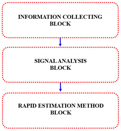
Figure 1.
Block diagram of the proposed rapid estimation method: the first block collects information on , , geolocation, and time stamp. The second block detects Primary Users (PU) and unused channels, stochastic and mathematical information, and Receiver Operation Characteristics (ROC). The third block applies the rapid method to estimate Television White Spaces (TVWS).
Nowadays, the United States of America is the only country that has released a TVWS spectrum for cognitive access in rural areas. The Federal Communications Commission (FCC) regulates its operation by using a data-based method. This approach consists of remote access to a database to know the transmitters and their characteristics in terms of location, antenna, transmit power, height, operation times, and others in order to ensure that there is no interference with PUs [8]. This fact can be seen as a good indicator, in the sense that probably other countries will consider releasing a spectrum according to their local regulations and needs.
The first application considered for TVWS was broadband access in sparsely populated areas by using cognitive radio techniques. With this purpose, the standard Institute of Electrical and Electronics Engineers 802.22 (IEEE 802.22) was approved in 2011 [9].
The presented paper is derived from the research detailed in [6]. Other interesting applications envisaged are the usage of TVWS in smart grid communications, as is explained in [10], or in Cognitive Vehicular Networks (CVN), as proposed in [11], or the indoor access to TVWS, also known as TV Gray Spaces (TVGS), detailed in [12,13]. Also, its application in rural communications networks with Wireless Regional Area Network (WRAN) has been mentioned in [14,15]. To materialize the abovementioned solutions, a REM complemented with a novel low-cost sensing technique would allow for identification of frequencies that may be used for DSA.
The motivation for this research is to take advantage of the unused radio spectrum to provide smart access to this much-needed resource. With this in mind, we proposed a method that estimates the presence of TVWS in a rapid and trustworthy manner, so that SUs can also be provided access to the spectrum demanding wireless services and applications. In the last years, the world has experienced impressive growth in wireless communication technologies and the appearance of new devices and services at an unprecedented pace. This fast change has created a never-seen-before demand for the electromagnetic spectrum in data transfer. The actual spectrum allocation shows a curious characteristic: we found parts in which the spectrum is crowded and some other parts in which it is underutilized [8]. Therefore, we can affirm that there is a duality of scarcity and wastage of this resource [2,3].
The rest of the manuscript is organized as follows. Section 2 provides a spectrum sensing overview for this research. Section 3 describes the data collection, analysis procedure, and signal representations. The rapid estimation method is detailed in Section 4, and the corresponding experiments and results are shown and analyzed in Section 5. Finally, Section 6 presents the conclusions and future work.
2. Spectrum Sensing Overview
An MSSS was implemented with the objective to sense the TV-UHF spectrum, as explained in [6]. By analyzing the results obtained therein, the authors realized the need for estimating TVWS in a rapid manner, for saving time, and for using open hardware and software tools. To conduct this research, we worked with data obtained from the TV-UHF band (500 MHz to 698 MHz). Spectrum samples were collected in the city of Windsor in Canada. We focused our efforts on identifying the available TVWS in the mentioned area.
Sensed Signals
Let us consider that the composite signal is the combination of the noise and the signals. To obtain accurate information regarding , two devices sensed simultaneously the TV-UHF spectrum, as seen in Figure 2; signal ws collected through the Winegard antenna [16] and processed with one RFE [7]. At the same time, another RFE device with similar characteristics and a 50 matched impedance replacing the antenna was used to sense the noise of the system [6]. As a result, both signals and were collected by the MSSS and processed as separated signals. Additionally, we saved the geographical coordinates to geolocate the readings. The MSSS scans at the 198-MHz bandwidths of the 500 MHz to 698 MHz TV-UHF spectrum had a separation of 1.76 MHz at a given time instance. This means that 112 samples were collected per RFE at each time instance. Along with the two RFE devices, we used a GPS device. Hence, a single reading consisted of a 112 signal power samples in dBm, 112 noise power samples in dBm, and 1 location-time stamp sample. The RFE devices took readings every 0.340 s, which implies that, for 1 minute period, we had (112 + 112 + 1) × (60/0.34) = 39,705.88 data samples.
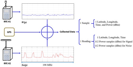
Figure 2.
TV-UHF spectrum samples were collected by using two Radio Frequency Explorer (RFE) devices in parallel, one to characterize the noise signal and another to collect the composite signal , together with a GPS receptor antenna to geolocate the readings. Each reading consisted of 112 samples for the composite signal and 112 samples for noise. The separation between two samples was 1.76 MHz, and all 112 samples covered 198 MHz, which is the TV-UHF bandwidth.
Our MSSS was composed of two RFE devices [7], from which signals were collected in parallel, compared, and processed to identify their characteristics. The used RF Explorer was a portable spectrum analyzer designed for the specific needs of digital radio frequency communication. The workflow was supported by the RF Explorer, including detection of expected transmission and power, automatically resolving Resolution Bandwidth (RBW), and sweep time and spectrum data calculations. It included functions such as real-time processing for adjusted signals, 3D spectrogram waterfall, Comma-Separated Values (CSV) export, and high-quality graphics, and it could work with Windows on a PC. This is a low-cost, open hardware-software, and portable device, the main characteristics of which are shown in Table 1.

Table 1.
RFE technical characteristics.
An example reading is represented in Figure 3, where panel (a) shows the noise signal and panel (b) represents the composite signal . Red peaks observed in panel (b) are the energy of the PU, which means that those channels were used by the incumbents. On the other hand, channels where the only signal sensed was the noise level was considered as unused channels or TVWS [17]. The energy detected in the TV-UHF channels is illustrated in Figure 3c. Readings collected in ten points are overlapped, allowing us to observe those channels with a higher probability of being used by a PU along the TV-UHF spectrum in the sensed area. In this case, the most used channels along the sensed geographical area were 21, 22, 26, 31, 32, 38, 41, 43, 44, 45, 49, and 50.

Figure 3.
Example measurements: (a) noise of the system, ; (b) composite signal sensed, ; and (c) the presence of the PU clearly observed when ten sampled points overlapped in order to illustrate the behaviour of the UHF TV spectrum in the sensed area.
3. Analysis of the Collected Data
With the MSSS mounted on a vehicle, the TV-UHF spectrum was sensed across a wide area. As mentioned before, it collected one reading every 340 ms and each reading was composed of 112 samples of , 112 samples of , their respective time stamp, and the latitude–longitude information. This procedure allowed us to create a spatiotemporal map of the sensed TV-UHF spectrum, as illustrated in Figure 4. To conduct this research, more than eight million samples were collected in the city of Windsor, Ontario, Canada. By scrutinizing the figure, we realize that there are different spectrum occupation rates according to the geolocation of the readings. The images framed in blue show the TV-UHF spectrum sensed, and we can observe therein peaks of energy that may correspond to PU signals distributed along different frequencies, so that those energy peaks identify the channels as being used. This irregular spectrum occupancy can be used for DSA to improve wireless communications services that require the electromagnetic spectrum.
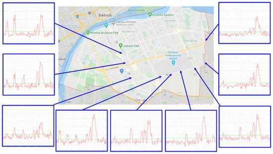
Figure 4.
Spatiotemporal map of the spectrum sensed in our area of interest.
The first action needed is to find used channels, and then, we need to identify their frequency and to get the geographical location. To do this, we must find an optimal threshold, denoted as T, to be used as a reference to decide the occupancy of a channel. At the same time, we can characterize the spectrum behaviour based on the taken samples. To calculate the best value for T, we have to consider that a higher value of T will reduce but that it also will increase , which will result in missed detection of real PU signals with low energy and will introduce errors in the results, as observed in Figure 5 with . On the other hand, a lower value for T reduces , which increases . This provokes noise peaks with high energy, which may be considered PU signals, again producing errors in the results, as is observed in Figure 5 with . It is a fact that the spectrum occupancy could be significantly changed when the threshold varies [18]. Here resides the importance to find an adequate value for T.
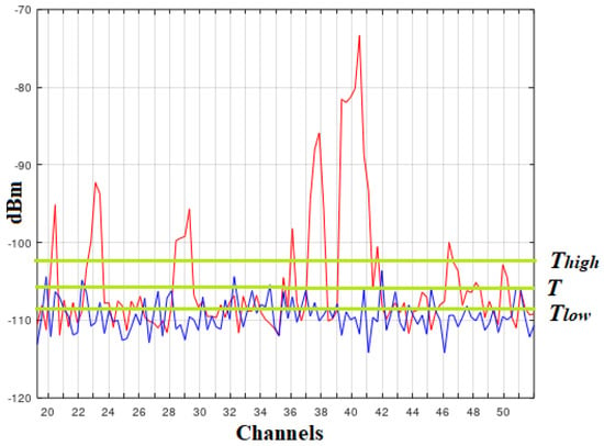
Figure 5.
Different values for threshold are plotted to show that produces missed detection of real PU signals and that produces some noise signals which are be considered PUs. In both cases, there are errors in the obtained results. An adequate value for T is plotted, which maintains enough distance from the noise floor to avoid false alarms and missed detection. This equilibrium is obtained when T considers a of .
Based on this, a good option to estimate T is explained in [6]. Now, let us consider that, for each reading, in which we measure , its mean value represents the noise floor that we will use as a reference to calculate our T explained:
with M as the margin that is obtained by using
where is the standard deviation of and is the Z-score that defines a equal to . The obtained T is represented in Figure 5.
Once the procedure to calculate T is defined, we wrote a script that compared each point read by the MSSS with T and its corresponding frequency in MHz. The sensed band ran from 500 MHz to 698 MHz, and each TV channel had a bandwidth of 6 MHz [1]. The script identified the points located above T and marked them as used channels; the points below T were considered TVWS. The output of the script is observed in Figure 6, where we visualize it with colours: in gray are the occupied channels, in white are the TVWS, and in yellow is channel 37 (608 MHz to 614 MHz), which is assigned to radio astronomy services. By comparing panels (a)–(c), we observe the changes from one to another location, where some channels are detected according to its geographical position.

Figure 6.
Channels detected as used are coloured in gray, whereas channels considered as TVWS are in white. Channel 37 is in yellow because it is assigned for other purposes. Panels (a–c) correspond to points 1–3, respectively.
Our next step was to complement the information observed in Figure 4 with the statistic parameters obtained from the sensed signals, i.e., and . From signals collected in parallel, i.e., noise and composite signal , we obtained their statistical characteristics as means (, ) and standard deviations (, ). We represented the signals as Probability Density Function (PDF) curves for a better understanding of the statistical analysis. It is important to notice that the signal follows a normal distribution as is demonstrated in [6] by applying the Kolgomorov–Smirnov Test (KST) [19]; hence, its PDF can be represented, as Figure 7a illustrates with blue line. On the other hand, the composite signal-sensed does not follow a normal distribution, as demonstrated in [6] by applying the KST. This phenomena is due to the multimodal nature of the composite signal sensed, as observed in Figure 7a in magenta dotted line.
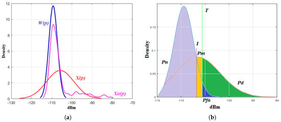
Figure 7.
Collected signal representation: (a) the Probability Density Function (PDF) of is represented in blue, the PDF of is plotted with a magenta dotted line, and the PDF of is plotted with red dotted line. Notice that and curves have the same means and standard deviations; (b) the normal PDF curves of , , and lines labelled as I and T delimit four areas under the curve (AUC). It is possible to identify in green, in blue, in orange, the in gray.
If we try to calculate the intersection point of and , it would be mathematically complicated due to the higher grade of the equation that represents the multimodal curve. This complexity is reduced if we replace with the normal curve by applying
where and are the means, and and are the standard deviation for and signals respectively.
Then, the assumed curve has the same mean and standard deviation values as , and it is illustrated in Figure 7a in red dotted line. This assumption reduces the complexity of the mathematical calculations while maintains the accuracy in our results. Once the assumption that can be replaced with is accepted, in the rest of the manuscript, we will refer to the composite signal as .
The next step was to define a threshold T located close enough to the noise floor to prevent missed detection and far enough to avoid false alarms. The value of T may be calculated by applying Equations (1) and (2), yielding the reference level to decide if the channel is used or not. On the other hand, normal PDF curves and , together with tentative T, defined four areas under the curve (AUC). Each of these areas represents a specific probability value as explained next. The probability of detection () refers to the signals above T and represents real PU signals detected. The probability of false alarm () accounts for noise peaks above T that may be misinterpreted as PU signals. The probability of noise () accounts for noise signals below T which are considered as noise. Finally, the probability of missed detection () accounts for undetected PU signals considered as noise. Both probabilities and will account for errors in the obtained results.
We need to consider an auxiliary line labelled as I, which projects the intersection point of ∩ on the power axis, as illustrated in Figure 7b. is represented as the yellow AUC delimited by I, , and T. Signals below I are the noise components of , and for that reason they are not considered as missdetected PU signals. To calculate , we can use
where I and T are the lateral limits to find the area under .
The value of T has to be calculated with the aim of reducing while maximizing , so that we use the statistical parameters of the noise signal to find its value. Hence, it can be defined by
where is the standard deviation of and is the Z-score. Let us consider that T has to fulfill
where is equal to I and has to consider that defines according to [20]. Based on this, a to obtain a = 3% has been used to reach accurate results, as is explained in [6]. On the other hand, T referred to the composite signal defined by
where is the standard deviation of and is the Z-score that defines the . By combining Equations (6) and (8), we find the value of as follows:
hence, after finding we obtain the for each point as observed in Figure 8a, which represents the ROC curve [21]. The outcome of this curve represents . By analyzing this curve and its variations as illustrated in Figure 8b, we can infer how overlapped the normal curves of and represented in Figure 7b are. This overlap depends on the number of detected PU.
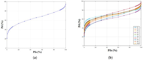
Figure 8.
ROC curve where is the input and is calculated: panel (a) shows a single ROC, and panel (b) shows the overlapped ROC curves from ten different points sensed.
As we can observe, the positions and patterns of the ROC curves are variable; these changes depend on how wide and overlapped the PDF curves of the and signals are. These variations are seen in Figure 9, where panels (a) and (d) represent the sensed signals where we can identify the presence of PU above T. In panels (b) and (e), the composite signal experiences an increment of its standard deviation (), which produces the expansion of the PDF curve, and as a logical consequence, the ROC curves shown in panels (c) and (f) modified their respective patterns.
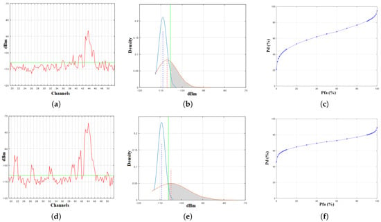
Figure 9.
Two-point readings are plotted, for which panels (a,d) represent the signal sensed. In panels (b,e), the PDF representations for and are presented, and panels (c,f) illustrate their respective Receiver Operation Characteristics (ROC) curves, where we can observe different patterns.
Accordingly, by understanding these variations, we can identify the behaviour of the sensed spectrum, can obtain related information, and can rapidly estimate the presence of TVWS in the analyzed TV-UHF band.
4. Proposed Rapid Estimation Method
With all the information collected and the analysis reviewed in previous sections, we developed a method for rapid estimation and visualization of TVWS. In Figure 10, we observe the diagram of the proposed REM. It shows the flow graph necessary to process the information obtained by using the MSSS. Once the signal of the , , and coordinates were collected and combined, these were fed into three blocks, namely, the Energy Detection (ED) block, the Statistical Analysis (SA) block, and the ROC Analysis (RA) block:
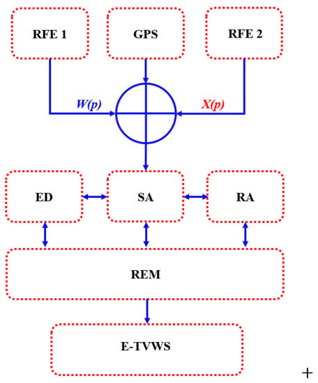
Figure 10.
Diagram of the rapid estimation method proposed that shows the data flow process: Data collected by the Mobil Spectrum Sensing Station (MSSS) are combined and fed into three sub-blocks, namely, the Energy Detection (ED), the Statistical Analysis (SA), and the ROC Analysis (RA). The output of these blocks is introduced in the Rapid Estimation Method (REM) block to obtain an estimation of the TVWS (E-TVWS).
- The ED block calculates the optimal value for T and identifies the channels in which PU signals are detected, marking them as used channels; otherwise they are identified as TVWS channels.
- The SA block obtains the statistical parameters of the sensed signals (i.e., , , , and ) used to identify and for each case. With this information, it creates a plot of the PDF curves.
- The RA block plots the ROC curves for each point sensed and identifies tendencies or patterns for each case.
The output of these three blocks are introduced to the REM block, where the results are combined to obtain an estimation of the TVWS (E-TVWS) channels available in the sensed point. To explain how the REM works, we used two well-differentiated sensed points; these are P1 that has the lowest PU detected, and P6 that has the higher PU detected. These points were taken from the ones shown in previous sections and will provide a didactic visual explanation to understand our proposed method.
4.1. ED Results
From the and readings taken by MSSS for each point and from the calculated T, our algorithm identifies those used channels, marked as PU, and those idle channels, marked as TVWS. The outputs of this sub-block are the channel and the number of PU and TVWS detected. This can be seen in Figure 11 for points 1 and 6. Panel (a) shows 10 used channels, which are 35, 38, 40, 41, 42, 43, 44, 45, 47, and 48, and this means 32.25% usage. Panel (b) shows 15 used channels, which are 20, 21, 26, 31, 32, 38, 39, 40, 41, 42, 43, 44, 45, and 49, and it means 46.87% usage. In this case, point 6 presents 50% more PU presence than point 1.
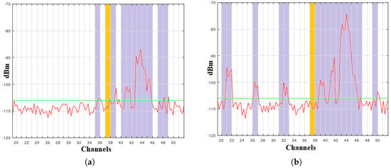
Figure 11.
Energy Detection (ED) results for points 1 and 6: (a) point 1, with 10 used channels, which are 35, 38, 40, 41, 42, 43, 44, 45, 47, and 48, means 32.25% usage and (b) point 6, with 15 used channels, which are 20, 21, 26, 31, 32, 38, 39, 40, 41, 42, 43, 44, 45, and 49, means 46.87% usage.
4.2. SA and RA Results
Sub-block SA obtains the and parameters given by and from the ED block, and with this information, it plots the PDF curves. This is shown in Figure 9b,e, where we can observe how and variate for each case. Additionally, we can infer that . To have a better idea of the variation in these parameters, Figure 12a illustrates the PDF curves for and of ten points represented and the value of the T calculated for each of them. We can observe that signals exhibit very low variation of its parameters. In the case of composite signals , the PDF curves exhibit higher variation. This difference occurs according to the number of energy peaks detected in the ED block.
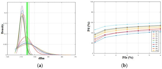
Figure 12.
Statistical Analysis (SA) results for example points: (a) PDFs of ten points that are overlapped. It is easy to observe that each point corresponds to different PDF curves. The shape variation is related to the number of energy peaks detected in the ED block. (b) ROC curves overlapped for points 1 to 10, where the horizontal axis scale has been modified to observe the variation in for a , shown by the green arrows.
With the information compiled from the MSSS, ED, and SA sub-blocks, the vs. the values are plotted to obtain the ROC corresponding to each point sensed. By comparing the ROC curves for points 1 to 10, we can observe a variation in the patterns, which is due to the different number of PUs detected in each case. This can be seen in Figure 12b, where the green arrows identify the variation of the corresponding to a .
The results of blocks , , and are presented and summarized on Table 2.

Table 2.
Tabulated results obtained from the ED, SA, and RA blocks.
4.3. REM Block
The REM block has been designed to find possible relationships with the obtained parameters to estimate TVWS in the TV-UHF spectrum of a specific geographical area. Its input consists of the data provided by the information collecting block and by the signal analysis block, as shown in Figure 1. To find E-TVWS, the measured parameters are taken from the information collecting block, and the calculated parameters are obtained form the signal analysis block. The REM block uses the sensed parameters and the calculated parameters to obtain the auxiliary parameters, as represented in Figure 13.
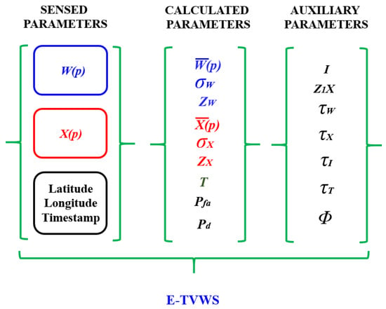
Figure 13.
REM parameters were used to find the estimation of the TVWS (E-TVWS), where sensed parameters are obtained by the MSSS, whereas calculated and auxiliary parameters are obtained by the signal analysis block.
To find a REM, we needed to use auxiliary parameters that allow us to understand the behaviour of the sensed signals and to obtain a numeric value to identify a possible relation among the sensed signal. These auxiliary parameters are described next:
- Parameter I is the first auxiliary parameter obtained, and it represents the projection line of the intersection point between and , as shown in Figure 7b. Parameter I marks the limit that separates the noise of the signal components of the composite signal , and it can be calculated using
- Parameter is represented by a line plotted in the upper limit of . To calculate its coordinates, we have to consider a Z-score that delimits 99% vs. 1% of the AUC in the right side of normal curve . This reference parameter will be very helpful to find the peak values of the composite signal , which usually are the PU signals. To determine the value of we can usewhere corresponds to the Z-score that defines an AUC of versus from right to left on the composite signal . We have defined parameters named () to identify the distance from to other parameter, as is explained in Table 3.
 Table 3. Distance measured from different statistical parameters.
 - Parameter refers to the distance measured from the and . It provides an idea of how spread out the composite signal in reference to noise signal is. If is bigger, this means that more s were detected in the signal.
- Parameter refers to the distance measured from the I intersection line and . It can be interpreted as the separation of the noise and the PU components in the composite signal .
- Parameter refers to the distance measured from the defined value of T and . It provides an idea of how spread out the AUC is.
- Parameter refers to the distance measured from the and , and it provides an idea of how spread out the composite signal is. By finding -, we can identify how close the and signals are. The closer they are, the less s are found.
- Parameter refers to the numerical ratio obtained when dividing the standard deviation for the composite signal to the standard deviation of the sensed noise, as expressed byThis parameter allows us to find the relation between the and with the purpose to know how spread out is to estimate the presence of . Based on this rate, we can affirm that, when the value of is lower, it means the less PUs in . On the other hand, when the value of is higher, it means there is less TVWS in the composite signal. The value for represents that the only signal present in the TV-UHF band is the noise . Here, we can use the Rose criterion explained in [22] and mentioning that a would be an adequate reference value to estimate the presence of and signals.
The auxiliary parameters explained are presented in Figure 14, where coloured arrows indicate the measured distance for each . Numerical values for the auxiliary parameters are summarized in Table 4, where parameters of the ten sensed points have been obtained by following the previously explained procedures.
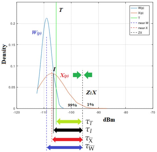
Figure 14.
In the plot that represents the PDF of the sensed signals, we draw a reference line named , which is defined by a Z-score that separates 99% vs. 1% of the AUC of . Additionally, we observe its distance from T, I, , and , denoted as , , and , respectively.

Table 4.
Auxiliary parameters used in the REM.
5. Results and Discussion
From each sensed signal, we calculated statistical parameters , , , and . We also calculated the optimal value for T minimizing . With the ROC curves, we then identified for each case. Additionally, we calculated the distance of the statistical parameters to the new reference point of . The obtained information was next used to find relationships among those parameters in order to identify patterns to provide us with new information.
Figure 15 illustrates the auxiliary parameters combined with the PDF curves for points P1 to P9. Here, we can visualize the variation of parameters for each location. The numerical values calculated for are represented in Table 4. When the obtained parameters are analyzed, we can identify two cases, as explained next:
where case I represents that and are more separated and there are more detected, whereas case II represents that and are closer and less PUs are using channels. By using to find how overlapped the sensed signals are, two extra parameters must be obtained, and these are and defined by
accordingly, corresponds to case I, and corresponds to case II.
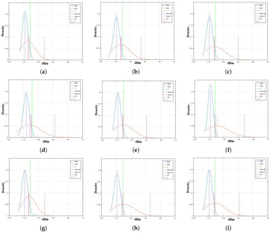
Figure 15.
PDFs of sensed parameters and showing calculated parameters , , and T as well as auxiliary parameters I and for points P1 (a) to P9 (i).
When this parameter variation is identified in readings of point P1 that contain the lowest number of PUs detected and comparing it with readings taken on P6, which have the maximum number of PUs detected, we can identify possible patterns that provide us with the baseline for a method to decide the presence of TVWS in other locations. However, we need to find information related to those extreme cases, i.e., only PUs in all channels and no PU detected at all.
5.1. Reference Channels
To obtain additional references for those extreme cases, we simulated two hypothetical scenarios. Scenario 1 presents the maximum number of PUs detected, and Scenario 2 detects noise signals only (no PUs detected). By analyzing these two extreme scenarios, we identified valuable references useful to find E-TVWS. Results from simulations are presented in Table 5. When these results are compared with the average of the tabulated values from Table 2, we can observe that there is no significant variation in terms of noise signal . For instance, varies in 0.12%, varies in −3.27%, I varies in −0.65%, and T varies in 0.22%. Those parameters related with composite signal showed considerable variation, and it can be considered when scrutinizing the elements to obtain E-TVWS.

Table 5.
Tabulated results obtained from simulated Scenarios 1 and 2.
In Scenario 1 with 32 PUs detected, the corresponded to 83.89%, whereas in Scenario 2, with no PUs detected, the corresponded to 3.70%. Then, is the main parameter to be considered. Figure 16 shows the extreme cases analyzed; in panel (a) are plotted ROC curves for Scenarios 1 and 2, and panel (b) shows the extreme ROC curves for Scenarios 1 and 2 and the for points P1 to P10, with green arrows showing limits for the extreme cases. It is easy to observe that, when the Pd increases (more PUs may be detected), the decrease.
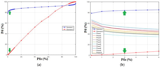
Figure 16.
Extreme cases analyzed: (a) ROC curves for Scenarios 1 and 2 in full scale; (b) extreme ROC curves for Scenarios 1 and 2 vs. the curves for points P1 to P10. Green arrows indicates the upper and lower limits for corresponding to 3% to find E-TVWS.
5.2. Confusion Matrix
With all the collected information, we create the two-dimensional Confusion Matrix (CM) observed in Figure 17, where we can visualize the relationship of the sensed signals [23]; here, we include , , , and . Rows represent the predicted condition and columns represent the observed (real) condition. This matrix helps us to identify characteristics and behaviour of the analyzed signals. Derived values from CM are presented in Table 6, where the Positive Predictive Values (PPV) [24] are calculated by using
and it represents the proportion of positive results obtained statistically that correspond to the . It describes the performance of the statistical method used. A high PPV value (≃) can be interpreted as an accuracy result. In this case, the average obtained is , and it means that the calculated for each case is accurate enough to be used as a reference parameter to find E-TVWS.
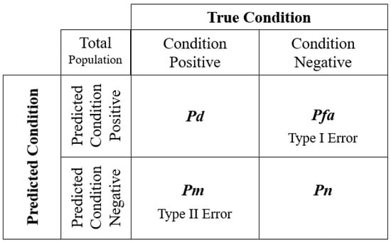
Figure 17.
Confusion matrix.

Table 6.
Confusion Matrix results for and .
5.3. PU Decision Matrix
The PU Decision Matrix (DM) to be also used here consists of a list of the TV-UHF channels, and it allows us to identify the most occupied channels by a PU as well as to rate those channels with a preferred order. The decision is based on PU presence criteria [25]. Here, we obtained the probability of channels that contain a PU signal, and for this purpose, our DM is composed of information obtained form the channels sensed.
For a visual representation of the DM, we plotted 32 channels numbered from 19 to 51 (channel 37 is not considered and is represented in yellow). The most likely channels to appear as used are in full blue colour; the coloured lines reduce its height according to the usage probability detected. Finally, we observe the less occupied channels in full white colour. By using this plot, we can estimate the amount of TVWS in the sensed area. The results are represented in a preferred order, where number 1 corresponds to the first option to be assigned as TVWS and number 6 correspond to the last option to be assigned as TVWS. Table 7 summarizes the DM output. For our purposes, we used channels with a PU occupation of less than of the sensed times. This means that only 10 channels can be assigned when we find E-TVWS with our REM model, and these are of the TV-UHF channels available in the Windsor–Essex region.

Table 7.
TVWS decision matrix: PU presence, channel numbers to identify them, percentage in the band of interest, and preferred order to be assigned.
The elements considered to find E-TVWS are based on the collected readings (i.e., data of points P1 to P10) and on simulated readings (i.e., Scenario 1 and Scenario 2), and they are listed below as a part of a PU DM:
- calculated from collected readings.
- calculated from Scenario 1.
- The value for .
- The value of .
- Preferred order to find E-TVWS.
5.4. Final Results
In this subsection, we include the information of points P1 to P10 analyzed using the REM. The results are listed in Table 8, where we present the probability of TVWS () calculated with the REM. These results are compared with the real number of unused channels detected in each point (). The variation column indicates the difference between the calculated and the detected . As we can observe, in the worst case, this variation reaches a and, in the best case, the variation reaches a value of . The average variation error found is . The maximum number of Detectable TVWS () is also presented, and finally, we can assign TVWS according to the preferred order mentioned in Table 7 by applying the PU DM.

Table 8.
Results of the tested point.
6. Conclusions and Future Work
6.1. Conclusions
A rapid method to estimate the amount of TVWS has been proposed, based on the probabilistic information obtained from the sensed signals. This method uses information collected by the mobile spectrum sensing station, which reads in a simultaneous manner the noise , the composite signal , the geographical coordinates, and the time stamp for each reading. From the collected information, the statistical parameters are obtained for both signals. With the statistical parameters obtained from the multimodal composite signal , which is not a normally distributed function, we traced a normally distributed function named . This assumption allowed us to reduce the complexity of the mathematical calculations to find the probability of detection . By combining the statistical and auxiliary parameters, the amount of TVWS was estimated. These E-TVWS are allocated in the TV-UHF band by following the preferred order identified in the decision matrix. The rapid estimation method was tested and yielded accuracy according to results obtained and verified. The average variation between the calculated and detected TVWS was in the range of . Built on open source resources, the proposed solution can be used to reduce both complexity and cost of TV-UHF spectrum sensing for estimating the presence of TVWS with acceptable accuracy results.
6.2. Future Work
Future studies could improve the proposed model by developing a script to read the and signals and to transmit in real-time the results of the TVWS estimation. This information would be shared with the Base Station (BS) and SU in need of accessing the spectrum to transmit data. In other words, when a low-cost network with enough accuracy senses the spectrum, trustworthy information related to the TV-UHF spectrum will be used to improve the DSA, without affecting the PU.
It is necessary to work in a model in order to know what would be the frequency reuse distances to implement a solution based on TVWS.
Author Contributions
D.C.-D.-W. collected and organized the data presented in this paper and analyzed the information. D.C.-D.-W. and S.A. wrote and reviewed the manuscript, analyzing the most relevant data. J.L.R.-Á. and K.T. reviewed and discussed the manuscript. All authors have read and agreed to the published version of the manuscript.
Funding
This research received no external funding.
Acknowledgments
This work was supported by the Secretaría de Educación Superior, Ciencia, Tecnología e Innovación (SENESCYT) of Ecuador and the University of Windsor. The authors thank the WiCIP Lab for providing all the equipment necessary to collect the information which is analyzed and discussed in this manuscript.
Conflicts of Interest
The authors declare no conflict of interest.
References
- International Telecommunications Union, ITU. Frequency Bands allocated to Terrestrial Broadcasting Services. Available online: https://www.itu.int/en/ITU-R/terrestrial/broadcast/Pages/Bands.aspx (accessed on 26 September 2019).
- Liang, Y.C.; Chen, K.C.; Li, G.Y.; Mahonen, P. Cognitive radio networking and communications: An overview. IEEE Trans. Veh. Technol. 2011, 60, 3386–3407. [Google Scholar] [CrossRef]
- Datla, D.; Wyglinski, A.M.; Minden, G.J. A spectrum surveying framework for dynamic spectrum access networks. IEEE Trans. Veh. Technol. 2009, 58, 4158–4168. [Google Scholar] [CrossRef]
- Liu, Y.; Ding, Z.; Elkashlan, M.; Yuan, J. Nonorthogonal multiple access in large-scale underlay cognitive radio networks. IEEE Trans. Veh. Technol. 2016, 65, 10152–10157. [Google Scholar] [CrossRef]
- Cordeiro, C.; Challapali, K.; Birru, D.; Shankar, S. IEEE 802.22: An introduction to the first wireless standard based on cognitive radios. J. Commun. 2006, 1, 38–47. [Google Scholar] [CrossRef]
- Corral-De-Witt, D.; Ahmed, S.; Awin, F.; Rojo-Álvarez, J.L.; Tepe, K. An Accurate Probabilistic Model for TVWS Identification. Appl. Sci. 2019, 9, 4232. [Google Scholar] [CrossRef]
- RF Explorer. RF Explorer Spectrum Analyzer. Available online: http://j3.rf-explorer.com/40-rfe/article/48-introducing-rf-explorer (accessed on 24 August 2020).
- Brown, T.X.; Pietrosemoli, E.; Zennaro, M.; Bagula, A.; Mauwa, H.; Nleya, S.M. A survey of TV white space measurements. In International Conference on e-Infrastructure and e-Services for Developing Countries; Springer: Cham, Switzerland, 2014; pp. 164–172. [Google Scholar]
- Kim, H.S. Location-based authentication protocol for first cognitive radio networking standard. J. Netw. Comput. Appl. 2011, 34, 1160–1167. [Google Scholar] [CrossRef]
- Orumwense, E.F.; Abo-Al-Ez, K. Exploiting TV White Spaces for Smart Grid Communications. J. Commun. 2020, 15. [Google Scholar] [CrossRef]
- Han, Y.; Ekici, E.; Kremo, H.; Altintas, O. Resource allocation algorithms supporting coexistence of cognitive vehicular and IEEE 802.22 networks. IEEE Trans. Wirel. Commun. 2016, 16, 1066–1079. [Google Scholar] [CrossRef]
- Bedogni, L.; Malabocchia, F.; Di Felice, M.; Bononi, L. Indoor use of gray and white spaces: Another look at wireless indoor communication. IEEE Veh. Technol. Mag. 2017, 12, 63–71. [Google Scholar] [CrossRef]
- Zhang, W.; Yang, J.; Guanglin, Z.; Yang, L.; Yeo, C.K. TV white space and its applications in future wireless networks and communications: A survey. IET Commun. 2018, 12, 2521–2532. [Google Scholar] [CrossRef]
- Aji, L.S.; Wibisono, G.; Gunawan, D. Analysis of white space coverage area radius to find the equilibrium point between DVB-T2 and IEEE 802.22 WRAN. In Proceedings of the 2017 International Conference on Electrical Engineering and Informatics (ICELTICs), Banda Aceh, Indonesia, 18–20 October 2017; pp. 173–178. [Google Scholar]
- Haider, A.; Rahman, R.; Noor, O.F.; Alam, F.; Huq, R.M. Towards an IEEE 802.22 (WRAN) based wireless broadband for rural Bangladesh–Antenna design and coverage planning. In Proceedings of the 2017 International Conference on Electrical, Computer and Communication Engineering (ECCE), Cox’s Bazar, Bangladesh, 16–18 February 2017; pp. 109–114. [Google Scholar]
- Winegard. Omminidirectional TV Antenna. Available online: https://d38mfwkkxtsm2m.cloudfront.net/documents/2452381.pdf (accessed on 24 August 2020).
- Saeed, R.A.; Shellhammer, S.J. TV White Space Spectrum Technologies: Regulations, Standards, and Applications; CRC Press: Boca Raton, FL, USA, 2016. [Google Scholar]
- Taher, T.M.; Bacchus, R.B.; Zdunek, K.J.; Roberson, D.A. Long-term spectral occupancy findings in Chicago. In Proceedings of the 2011 IEEE International Symposium on Dynamic Spectrum Access Networks (DySPAN), Aachen, Germany, 3–6 May 2011; pp. 100–107. [Google Scholar]
- Massey, F.J., Jr. The Kolmogorov-Smirnov test for goodness of fit. J. Am. Stat. Assoc. 1951, 46, 68–78. [Google Scholar] [CrossRef]
- Chen, Y.; Oh, H.S. A survey of measurement-based spectrum occupancy modeling for cognitive radios. IEEE Commun. Surv. Tutor. 2016, 18, 848–859. [Google Scholar] [CrossRef]
- Brown, C.D.; Davis, H.T. Receiver operating characteristics curves and related decision measures: A tutorial. Chemom. Intell. Lab. Syst. 2006, 80, 24–38. [Google Scholar] [CrossRef]
- Watts, R.; Wang, Y.; Winchester, P.A.; Khilnani, N.; Yu, L. Rose model in MRI: Noise limitation on spatial resolution and implications for contrast enhanced MR angiography. Intl. Soc. Mag. Reson. Med. 2000, 4, 462. [Google Scholar]
- Stehman, S.V. Selecting and interpreting measures of thematic classification accuracy. Remote. Sens. Environ. 1997, 62, 77–89. [Google Scholar] [CrossRef]
- Fawcett, T. Introduction to Receiver Operator Curves. Pattern Recognit. Lett. 2006, 27, 861–874. [Google Scholar] [CrossRef]
- Yang, J.B.; Xu, D.L. On the evidential reasoning algorithm for multiple attribute decision analysis under uncertainty. IEEE Trans. Syst. Man Cybern. Part Syst. Hum. 2002, 32, 289–304. [Google Scholar] [CrossRef]
© 2020 by the authors. Licensee MDPI, Basel, Switzerland. This article is an open access article distributed under the terms and conditions of the Creative Commons Attribution (CC BY) license (http://creativecommons.org/licenses/by/4.0/).