The methodology of this paper follows four major tasks, including: (1) data pre-processing, (2) algorithms configuration, (3) design of workflows, and (4) scoring metrics for the designed workflows. Each task is then divided into necessary sub-tasks, as shown by the ordered bullet points.
2.1. Data Pre-Processing
We have used our domain expertise in the oil and gas industry to preserve the statistical properties of features and conduct necessary data transformation, before applying any ML workflow. The original dataset used for this study involves data collected from 1567 unconventional gas wells and 121 recorded features. These features are categorized into seven groups: Well API, Trajectory, Perforation, Injection schedule, Logging and Geomechanics, Operations, Production, and Others. A summary of the features in the dataset is presented in
Table 1. All relevant pre-processing techniques are briefly described below.
- (a)
Primary scanning
The first subtask in data pre-processing is the primary scanning process, which removes all features that have an amount of missing data exceeding 20% of the total amount of wells, i.e., all wells that miss production and/or trajectory data are removed from the dataset.
- (b)
Detachment of characteristic features
Next, a feature that considers characteristic inputs such as well number or pad/field number is identified. These features are not necessary for later tasks such as handling missing values, removal of outliers or applying ML models. Therefore, these characteristic features are detached from the data and extracted separately for further analysis, e.g., type well generation or re-frac candidate selection.
- (c)
Detachment of unchangeable features
In addition to characteristic inputs, some features hold numerical data, however, data of these features are unchangeable at the field, for example, well locations or operation conditions. Therefore, similar to the characteristic features, this information is also detached from the data and extracted separately for further analysis.
- (d)
Handling of missing values
Some features have missing data in part of the well. Instead of removing the feature if the missing data is no more than 20% of the data, we have tried to estimate that using different imputation techniques. K Nearest Neighbour (KNN) imputation technique [
5] is used to fill in values at all missing locations in the data. A further test of the imputation technique is additionally conducted to verify its performance accuracy. This accuracy-test randomly removes a portion of the known values from the dataset, followed by performing the imputation technique, and eventually measures the accuracy between the imputed data and the removed portion of the known values. An accuracy of 85% is recorded for the test, which quantifies the credibility of the KNN imputation technique used in this study.
- (e)
Data transformation
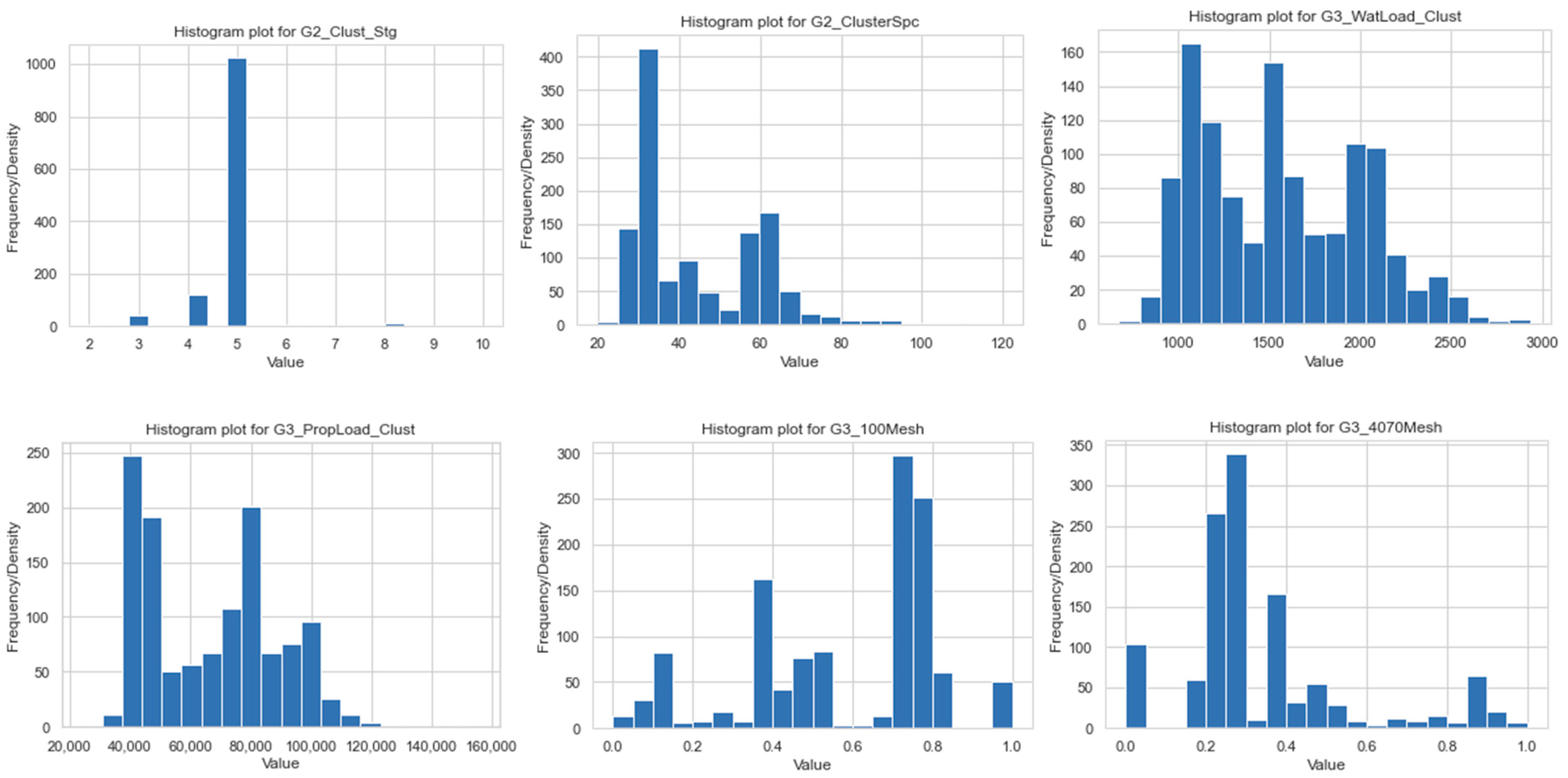
Most of the machine learning algorithms tend to perform better if features preserve the normal distribution due to the underlying Gaussian assumption and the application of central limit theory, which requires that the dependent feature is normally distributed to be able to express them as the sum of numbers of independent variables. However, statistical distributions of several features in the studied dataset do not comply with normal distribution. Consequently, quantile transformation is performed multiple times on each feature (due to the stochastic nature of the procedure) and the results are averaged to convert the original distribution of features to become normally distributed before further pre-processing and modeling work.
- (f)
Removal of outliers
After processing the imputation of missing values and data transformation, outliers are detected and removed from the dataset. In general, for every feature in the dataset, data points that fall out of three standard deviations (after being transformed to Gaussian distribution) are considered outliers to be removed. However, all detected outliers are re-analyzed depending on the physical context of the features and cross-checked with the history of the field before the final removal decision, to preserve physical characteristics of the original data and high- and low-end exploratory cases deployed in the field. After performing outlier removal, the dataset dimensions are reduced from 1303 wells, 41 features to 1290 wells, and 41 features. Since outlier removal is the final step in the pre-processing sequential tasks, the finalized data, which is tested for all designed workflows in this study, has 1290 wells and 41 features.
2.2. Algorithms Configuration
There are different algorithms available for model selection and hyperparameter optimization that have been used in different machine learning algorithms. Here we are summarizing these techniques and then proposing the optimum integration of the algorithms in a new workflow to be applied in our database.
- (a)
Grid/random search
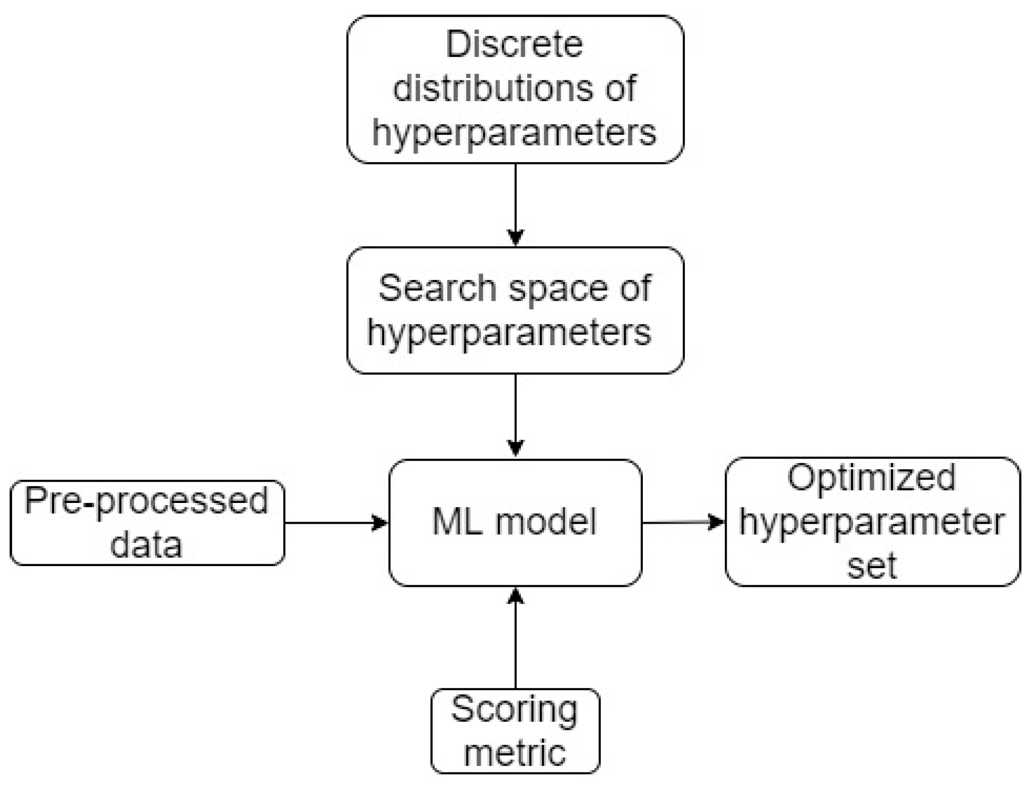
Grid search or random search are two classical approaches that aim to find the optimal hyperparameters for a given ML model. Grid search processes search for optimal hyperparameters through four steps, including importing pre-set discrete distributions of hyperparameters, generating all possible combinations of hyperparameters (which is defined as the search space), testing all combinations of hyperparameters for the given ML model, and eventually providing the optimal combination that maximizes/minimizes the selected scoring metric. Random search processes for optimal hyperparameters also follow similar four steps as grid search algorithms. However, there are two key differences between random search and grid search. Pre-set continuous distributions of hyperparameters are imported to replace discrete distributions, and a random number of combinations from the search space are processed through the optimization in replacement of all possible combinations. As being described, both grid search and random search conduct their aims (i.e., find the optimal hyperparameters for a given ML model) using a random procedure, which leads to the fact that results from previous combinations do not provide any insights for a directive selection of upcoming combinations.
- (b)
Bayesian search and optimization
Bayesian search is an algorithm that is similarly known to optimize the hyperparameters for a given ML model as grid/random searches. The notable difference in Bayesian search is its directive approach in selecting the next combinations of hyperparameters using the results obtained from the previous combinations, whereas grid/random searches, as mentioned, do not have this characteristic. In this study, Bayesian search is performed using Bayesian optimization, which is a narrow field of Sequential Model-Based Optimization (SMBO) [
6]. In SMBO, the procedure is as follows:
- -
Import the distributions of hyperparameters to be searched.
- -
Import the objective function (commonly the loss function), the acquisition function (as a criterion for selecting the next set of hyperparameters from the current set), and the surrogate model.
- -
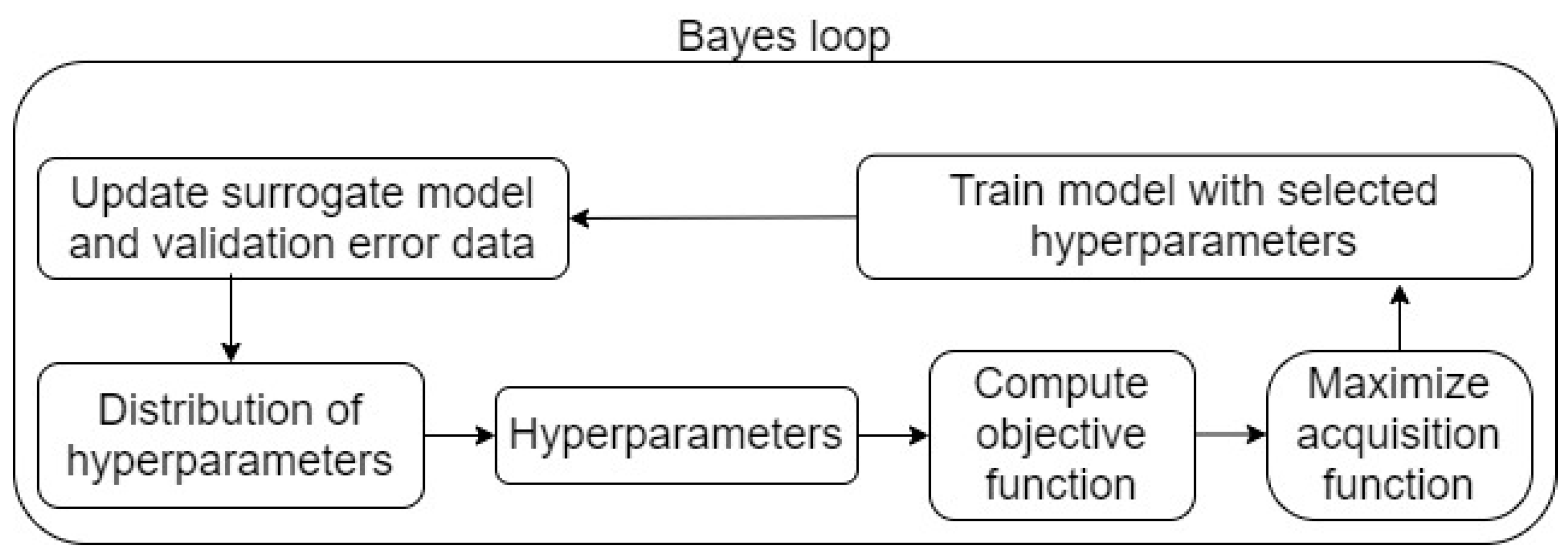
Within a set of hyperparameters selected from the imported distributions, the procedure is conducted using a Bayes loop, as follows:
Fit the surrogate model.
Compute the objective function and maximize the acquisition function.
Apply the model with the intended set of hyperparameters to the data.
Update the surrogate model to decide which set of hyperparameters from their distributions to select next.
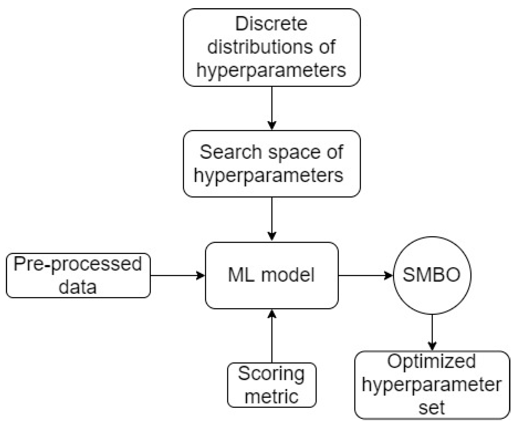
The Bayes loop is presented in
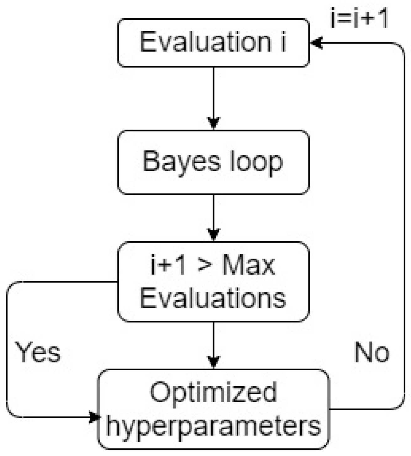
Figure 1. The procedure is presented in
Figure 2 as a general schematic for SMBO. In SMBO (and Bayesian optimization as focused on in this study), the surrogate model and acquisition function are two essential key functions in the Bayesian evaluation loop. In this study, the Gaussian Process is selected as the surrogate model, albeit Tree-structured Parzen Estimator (TPE) is another comparable option [
7]. Gaussian Process is a random process for a set of random variables
, where their joint distribution is Gaussian and formulated as:
where
is the mean function (
=
and
is a covariance (kernel) function. If
are found to be similar by Gaussian covariance function, then
. Knowing the training dataset
in this case hyperparameters and their functional values
, i.e., Gaussian random function, the posterior probability distribution function
can be obtained, which can be used to predict a new set of hyperparameters
. The posterior distribution function is also gaussian and can be obtained using the gaussian conditional distribution function. To optimize the hyperparameters, the objective function
will be sampled from
samples drawn previously, as follows:
where
EI is an acquisition function, i.e., Expected Improvement acquisition function (
EI) which is widely used in the industry. For a hyperparameter set
, EI is defined as follows:
In Equation (3),
is the most optimal value of the objective function (updated) for the best hyperparameter set
. To optimize the hyperparameter set
the Bayesian optimization algorithm is used. The nature of EI, as presented in Equation (3), always directs to select the best hyperparameter set. More advanced explanations for SMBO, Gaussian Process, EI, and a combination between Gaussian Process and EI in a Bayesian evaluation loop can be found elsewhere [
8,
9].
Even though Bayesian optimization has commonly been used as a search algorithm for hyperparameter optimization, it can also be used for searching an optimal ML model. However, this specific use of Bayesian optimization is limited to a few specific cases, as detailed in [
7].
In this paper, Bayesian optimization is used for hyperparameter optimization and a tree-based programming tool (TPOT) is used to search for the optimal machine learning model, which is more powerful than Bayesian optimization. TPOT inherits several strengths from Genetic Programming. Both TPOT and Genetic Programming are further described below.
- (c)
Genetic Programming
Genetic Programming (GP) is a pool of algorithms that closely relates to Genetic Algorithms (GA) and falls under the terminology Evolutionary Algorithms (EAs) [
10]. GP was invented and has been evolved to solve general or field-specific problems in science, medicine, and engineering.
An example problem in which GP effectively excels should have two intrinsic properties. First, there should be more than one unique solution that can fit the problem, and second, although an immediate deterministic solution is unavailable, an initial set of possible solutions are known. Based on the two aforementioned properties, solutions shall be optimally and appropriately approached by the sequential selection, starting from the known initial set of possible solutions.
In GP, final solution(s) are formed using sequential reproduction processes through generations to direct an optimal fit to the problem. At a generation, a sequential reproduction starts from the selection of the best solutions (commonly defined as individuals) within the generation’s population (commonly referred to as the set of possible solutions at that generation). The selected individuals are determined using a fitting criterion (i.e., a fit function) and are further grouped as a new population for crossover. Crossover is a main reproduction operator in GP/GA [
11], which processes two selected individuals (commonly named as parents), swaps portions of their structures to form new individuals (commonly named as offspring). In case the outcomes from the crossover are determined as a successful fit for the problem, the new population’s data is extracted and passed as the new generation’s population. Otherwise, the outcomes from the crossover (as exact copies from their parent individuals) are further grouped for the mutation before being passed as the new generation’s population. The mutation process is proposed to maintain diversity in a generation and expand the possibility of better results from the crossover process in the next generation. Mutation processes one selected individuals by randomly changing a portion of its structure to form a new individual.
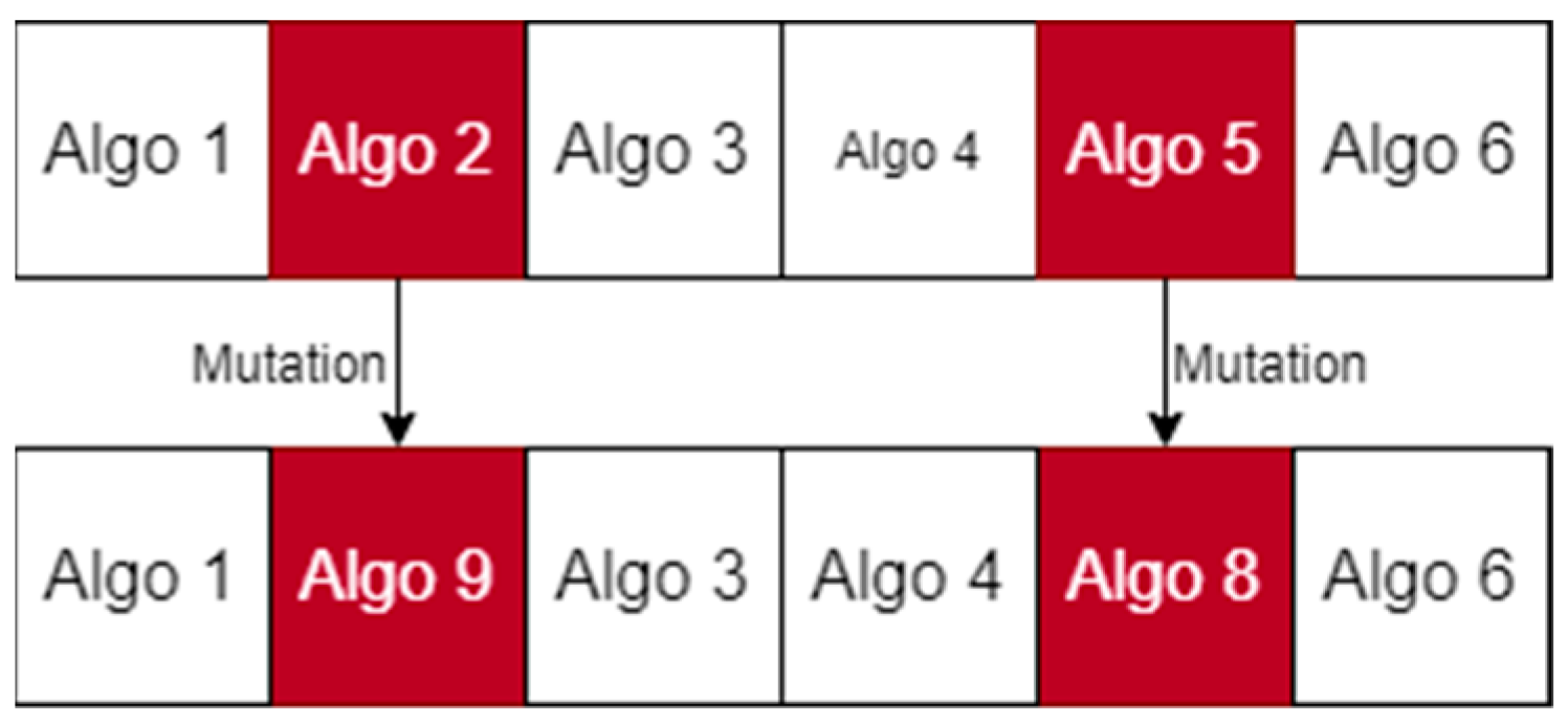
Under the context that an individual in this study is formed as a set of algorithms in sequence, crossover and mutation can be explained, as shown in
Figure 3 and
Figure 4. In these figures, “Algo” is an abbreviation for an algorithm in a ML pipeline (as in
Figure 3 and
Figure 4). In
Figure 3, the crossover swaps the structure of the two individuals at the indicated double arrows (i.e., known as “single-point” crossover algorithm) and produces 2 new ML pipelines. In
Figure 4, mutation chooses Algo 2 and Algo 5 in the individual’s structure and changes them to Algo 9 and Algo 8 (i.e., known as “flipping” mutation algorithm) to produce a new ML pipeline.
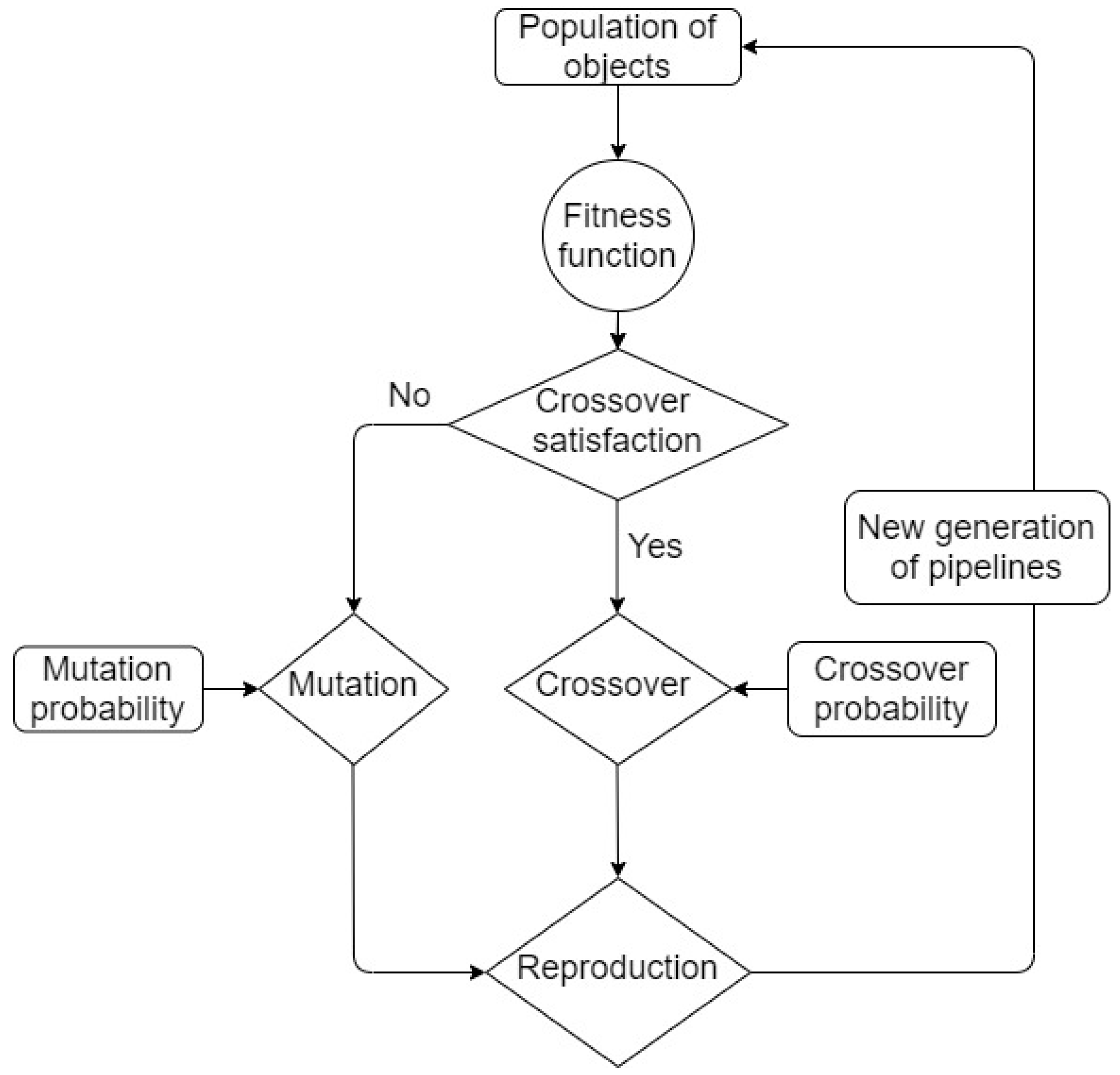
GP is inherited and functions based on the core characteristics of the biological reproduction process, including the characteristic that crossover and mutation are processed in GP with probabilistic nature. A schematic of a general GP algorithm is presented in
Figure 5. Additional explanations and more details for GP/GA, crossover, and mutation can be found elsewhere [
3].
- (d)
Tree-based Pipeline Optimization (TPOT)
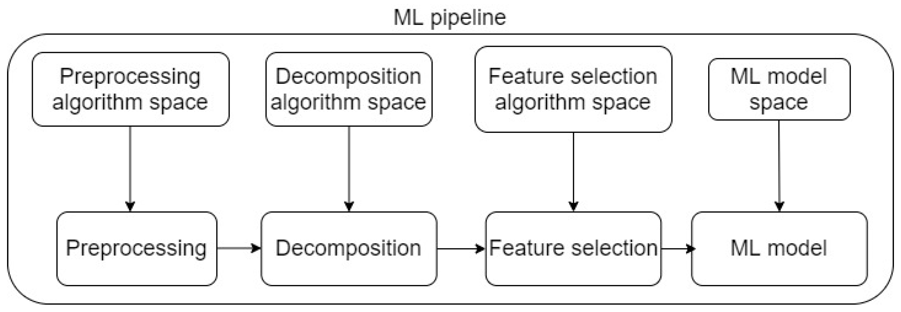
TPOT inherits characteristics from GP/GA and applies GP/GA algorithms for Automatic Machine Learning (AML) problems, which exhibit high levels of complexity and practicality for high-dimensional datasets. The foundation in TPOT is based on standard ML tasks for all ML studies, which include pre-processing, data decomposition and transformation, feature selection, and eventually modeling. This set of tasks in TPOT is defined as a machine learning pipeline. The schematic of a ML pipeline in TPOT is presented in
Figure 6. Provided the fact that there exist numerous pre-processing techniques, data decomposition algorithms, feature selection techniques, and especially ML models, consequently, there exist numerous possible pipelines as suitable solutions. Additionally, a deterministic solution that is immediately optimal is challenging, as testing for all possible pipelines is impractical. Based on the nature of GP/GA, the best machine learning pipeline (as the final solution) is the one among the final generation that satisfies the optimization criteria (determined by one or more scoring metrics). In other words, TPOT implements GP to find the best machine learning pipeline through generations of searching, starting from an initial population of different pre-processing techniques, data decomposition algorithms, feature selection techniques, and especially ML models. A currently notable application of TPOT in bioinformatics can be found in [
8,
12].
TPOT directs the selection of the best machine learning pipeline, as follows:
Within a generation’s population, each possible pipeline is evaluated for its fitness to the problem.
Using the fitness results, the best pipelines are stored as a new population to process the crossover (impacted by crossover probability) and create the next potential generation of pipelines.
All created pipelines are tested for their performance in the provided data, using pre-set scoring metric(s).
In case the result is plausible, the created pipelines’ data is passed to the next generation.
In case no created pipelines perform satisfactorily, a mutation is performed between the created pipelines to expand the number of pipelines (impacted by mutation probability), and data from all created pipelines (by both crossover and mutation) is passed to the next generation.
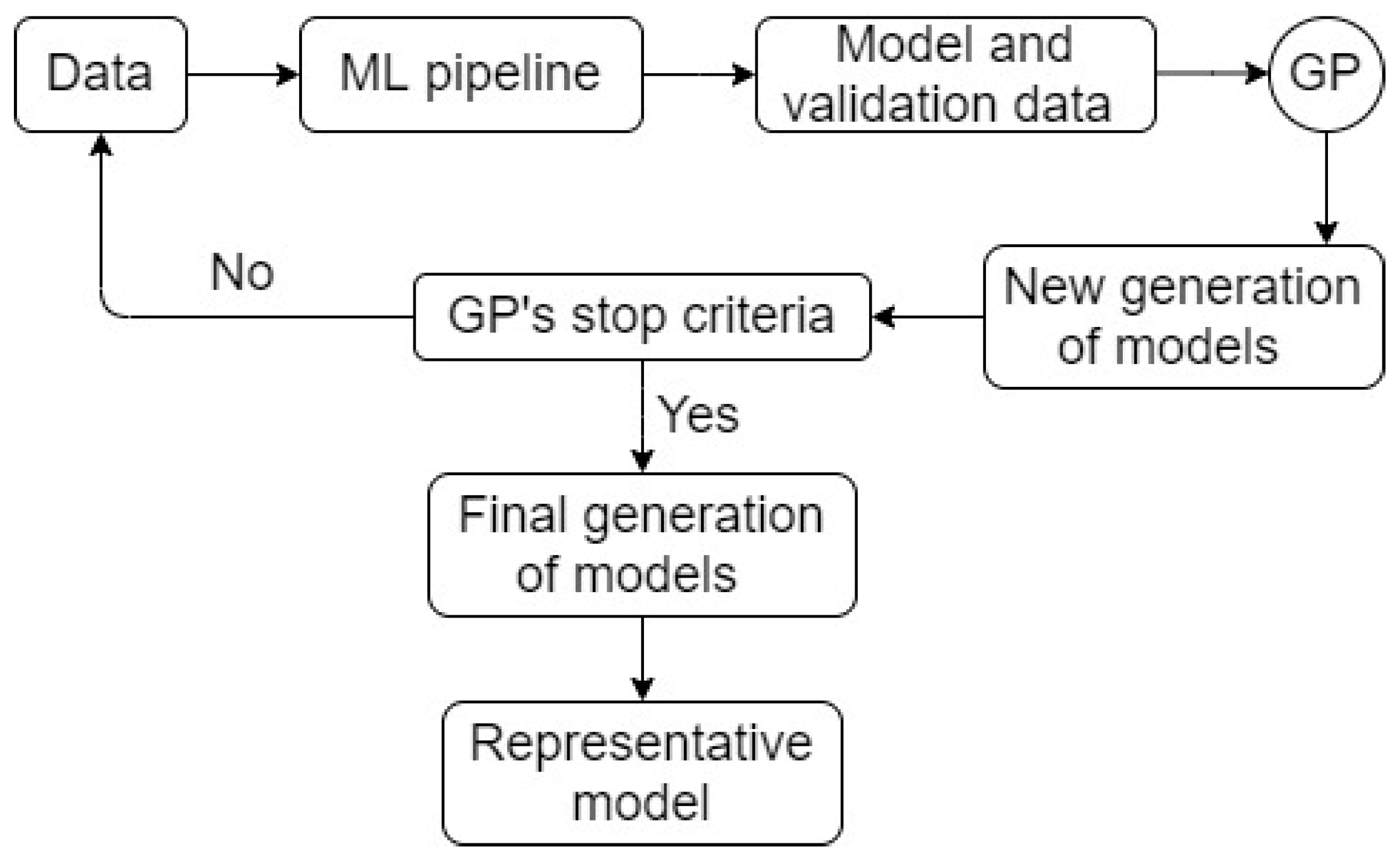
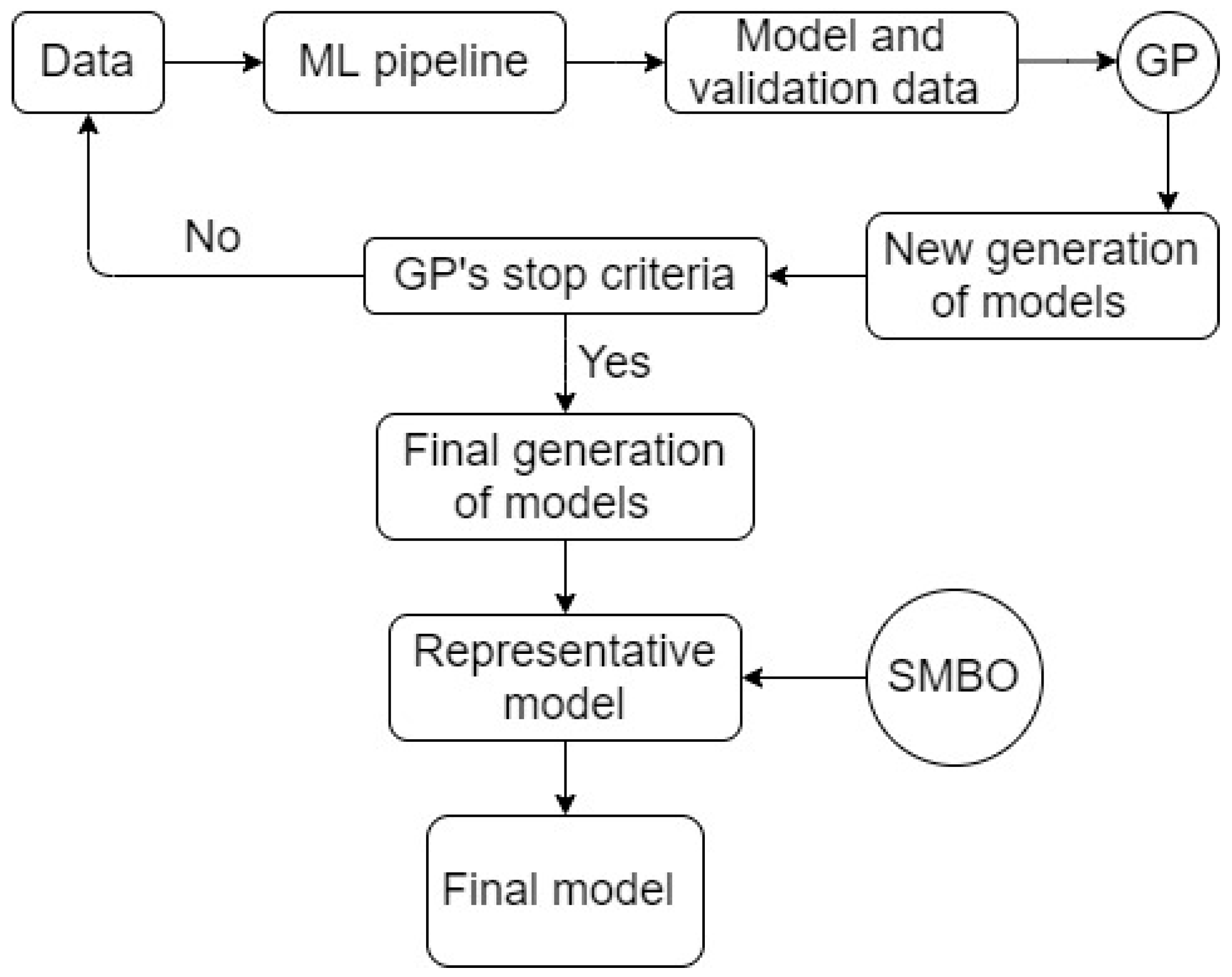
TPOT is terminated when the stop criteria are satisfied (commonly set as the maximum number of generations reached). The representative pipeline from the final generation’s data is the most suitable machine learning pipeline for the given problem.
A schematic of TPOT is presented in
Figure 7. TPOT was proven to perform significantly better than classical statistical analysis and manual machine learning practices [
8]. Additional explanation of TPOT, its relevant development, algorithms, and especially common GP settings in TPOT can be found elsewhere [
3,
8].
2.3. Design of Workflows
In this paper, a new hybrid workflow is designed and tested against common practices using real filed data obtained from more than 1500 gas wells. The studied workflows are numbered in order as 1–4, and their descriptions are detailed as follows:
Workflow 1 (lowest level of complexity): This workflow is the most commonly used machine learning workflow, in which the model is readily pre-defined (i.e., manually selected), and the core aim is hyperparameter search [
13]. The search process for hyperparameters in workflow 1 is performed using grid/random searches. A schematic of workflow 1 is presented in
Figure 8.
Workflow 2 (higher level of complexity compared to workflow 1): This workflow is the more advanced version of workflow 1. Its machine learning model is also manually selected and hyperparameter search remains as the central aim. However, hyperparameter search in this workflow is performed using Bayesian search and optimization. A schematic of workflow 2 is presented in
Figure 9.
Workflow 3 (higher level of complexity compared to workflow 2): The central aim of this workflow is to find an optimal machine learning model using TPOT. Being inferred in the TPOT’s description, the final and optimal machine learning model is searched from a population of well-known machine learning models with various complexity levels (linear/logistic algorithms, Support Vector Machines, Random Forest, Randomized Extra Trees, Gradient Boosting, Extreme Gradient Boosting, Neural Network). Schematic of workflow 3 is readily presented in
Figure 6 and
Figure 7.
Workflow 4 (highest level of complexity within all workflows—a “hybrid” workflow): the central aim of this workflow is a combination of finding an optimal machine learning model and searching for its optimal hyperparameters. Workflow 4 was proposed and studied to integrate the key strengths of both TPOT and Bayes optimization. TPOT itself is a powerful set of algorithms used to focus on extracting an optimal machine learning pipeline in a modeling context, however, this tool does not focus on hyperparameter search for a machine learning model. As a result, Integration of Bayesian optimization with TPOT helps to increase the robustness of the machine learning pipeline optimization from the beginning (pre-processing) to the end (hyperparameter tuning).
For an ordered description, TPOT is initially applied in searching for an optimal ML model (similarly to workflow 3). Results from TPOT (the optimal ML model generated and its hyperparameters) are further processed through Bayesian search and optimization for searching for the best possible hyperparameters. The schematic of workflow 4 is presented in
Figure 10.
2.4. Scoring Metrics for the Designed Workflows
Pearson correlation (i.e., R2 correlation) and Mean Square Error (i.e., MSE) are selected as two scoring metrics to evaluate the performance of all studied workflows. These metrics are selected due to their compatibility with all the levels of complexity in the designed workflows. A minor modification of MSE to negative MSE is conducted, however, this modification merely increases seamlessly between pre-processing and modeling for a few runs and does not impact modeling evaluation.
- ○
Pearson correlation (R2 correlation)
Pearson correlation (i.e., correlation of determination), for a sample size
, is computed as follows:
- ○
Mean Square Error (MSE)
Mean Square Error for a sample size
is computed as follows:
In Equations (4) and (5), is the known value, is the predicted value from the model, and is the average value of the given data.
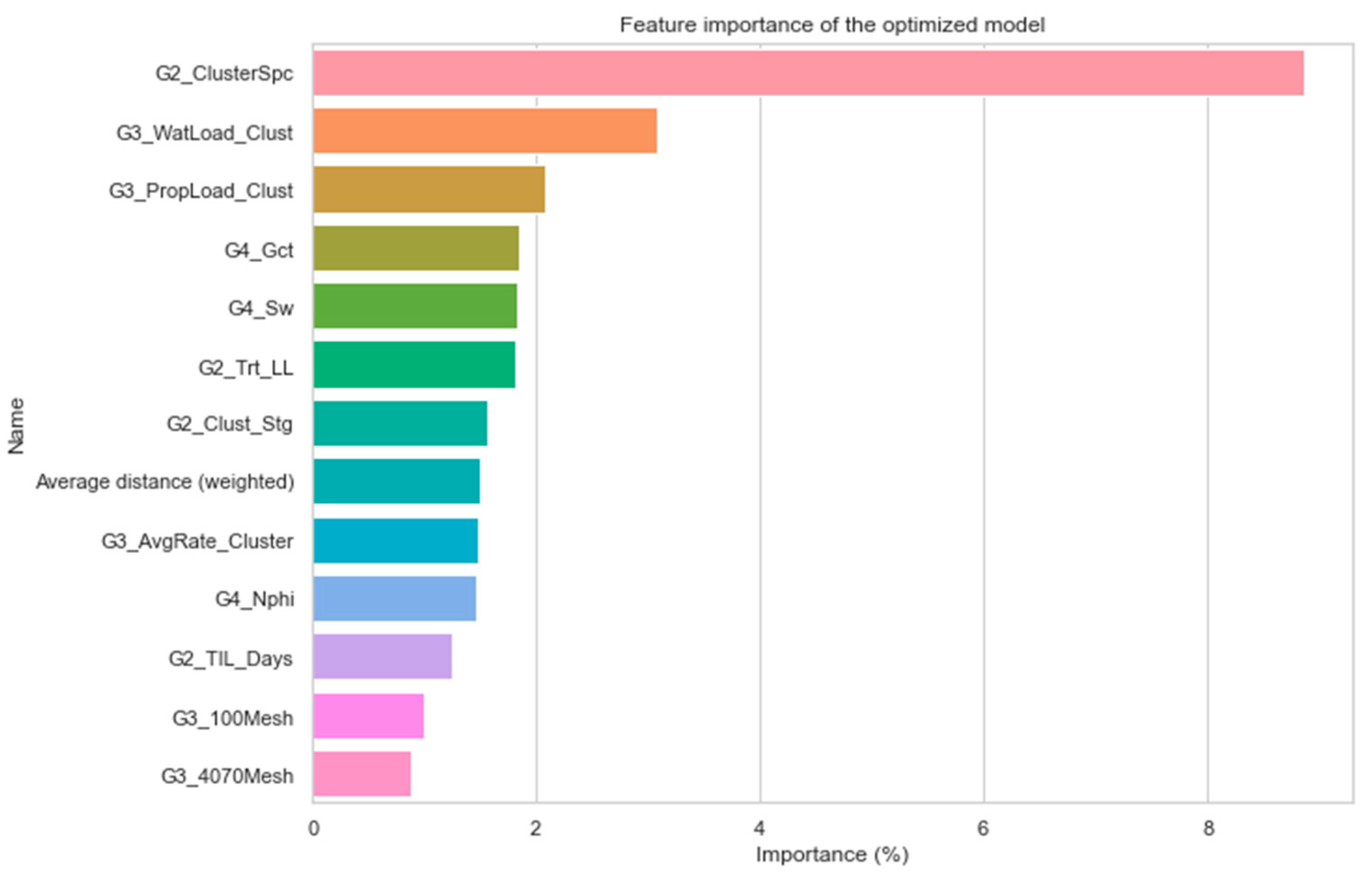
As aforementioned, workflow 4, which is a hybrid workflow between TPOT and Bayesian optimization, is further applied to real-field, high-dimensional data in the Marcellus Shale reservoir. The data contains 1567 wells and 121 features including drilling, completion, stimulation, and operation. In addition to the application of the proposed workflow to understand physical patterns in this dataset, the optimized model from the workflow is further implied in other studies for unconventional reservoir development optimization, including stimulation design, type well generation, and re-frac candidate selection. Workflow 4 exhibits superiority compared to the other studied workflows in this paper, and its superiority is detailed in the next section.
