A Generation-Weighted Modelling Framework for Life Cycle Assessment of Low-Carbon Electricity Mixes: Scenario Simulation, Boundary Diagnostics and Regional Proxy Analysis

Abstract

Installed-capacity shares are widely used to describe power-sector transition, but per-kWh life cycle assessment (LCA) depends on delivered generation. This study develops and tests a static, annual-average generation-weighted structural diagnostic framework linking capacity-to-generation conversion, technology impact factors, scenario simulation, uncertainty analysis, optimization-boundary diagnostics, and regional proxy analysis. The lcpy Simple LCA capacity mix supplies six pedagogical S0–S5 stress-test scenarios, while UK official capacity and generation observations provide a 2020–2024 observational backcast. Relative to raw capacity shares, fixed 2024 capacity-factor weighting reduces mean generation-share error by 60.1%, and a prior-year capacity-factor model reduces it by 72.3%; these improvements are interpreted as arithmetic and structural evidence, not as evidence of dispatch-model forecasting skill. In the scenario set, generation weighting lowers GWP100 by 13.55–22.59%; the low-fossil S2 scenario gives the lowest GWP100, 0.09011 kg CO₂-eq kWh⁻¹, 50.01% below S0, and remains lowest in the tested climate-change sensitivity analyses. Multi-indicator rankings are less stable, with S2, S3, and S4 forming a low-burden group rather than a method-invariant optimum. Applying the same weighted-sum calculation to 2024 generation structures for China, the UK, and the EU gives a central-proxy China GWP100 of 0.7497 kg CO₂-eq kWh⁻¹; this is a proxy-based structural diagnostic, not a validated regionalized LCA. The results relocate the assessment focus from installed capacity to delivered generation while identifying time-varying utilization and region-specific inventories as necessary extensions.

1. Introduction

Power-sector decarbonization is often reported through installed low-carbon capacity, yet the environmental burden of one kilowatt-hour is determined by delivered electricity, and wind, solar photovoltaic (PV), hydropower, nuclear power, natural gas, and coal differ in capacity factor, dispatch role, resource availability, and life-cycle inventory profile. A capacity-based representation can therefore overstate the environmental effect of technologies that are installed but generate less electricity or understate the effect of technologies that operate at high utilization. Comparative life cycle assessment (LCA) studies show large differences among electricity-generation technologies across climate-change, resource-use, human-health, and ecosystem indicators [1,2,3]; low-carbon technologies also carry non-negligible upstream burdens from materials, infrastructure, land occupation, and end-of-life processes [4]. Recent reviews comparing conventional, nuclear, and renewable technologies confirm that such cross-indicator differences persist in current life-cycle inventories [5]. Electricity-transition modelling must therefore quantify the delivered generation that low-carbon capacity contributes and the high-impact generation it displaces, in addition to the installed capacity itself.

LCA provides the functional-unit and system-boundary discipline needed to analyse this question, but the modelling choices within electricity-mix LCA remain consequential. ISO 14040 and ISO 14044 establish the general LCA framework [6,7], and early SETAC practice helped translate this framework into technology-comparison studies [8]. This practice has since grown into a diversified and still-expanding methodological field, as bibliometric analyses of LCA research trends document [9]. Coal-power LCA demonstrated that upstream fuel extraction and transport can be decisive for electricity impacts [10], while cross-technology reviews showed that no single generation technology is environmentally neutral across all indicators [2,3]. Upstream mining and fuel supply remain major impact contributors in current coal-power assessments [11]. Later methodological tools broadened the modelling space: TRACI v2.1 expanded midpoint assessment beyond climate change [12]; ecoinvent improved the traceability and consistency of background inventories [13]; and open tools such as Brightway (bw2data 4.7, bw2calc 2.4.0) and lcpy (v1.0.0) made parameterized and scenario-based LCA more reproducible [14,15]. Integrated assessments of electricity-supply scenarios then shifted the field from isolated technology comparison toward electricity-mix modelling [16]. Structured comparisons of current LCA software likewise show that open tools now support end-to-end reproducible workflows [17]. These studies establish the basis for scenario LCA, but they also show that a model can be misleading if generation shares, indicator weighting, and boundary assumptions are not made explicit.

Recent work further shows that electricity-mix LCA is sensitive to spatial, temporal, and accounting choices in addition to technology factors. Reviews of spatiotemporal electricity LCA indicate that annual average mixes can conceal regional and intra-annual variation [18]; dynamic electricity LCA shows that changing generation profiles can alter environmental effects within the year [19]; and electricity-accounting studies warn that inconsistent regional averages and accounting boundaries may create double counting or misleading allocation [20]. Regional environmental-impact curves and prospective LCA tools extend this point by showing that location, time, and future background assumptions can shift the interpretation of electricity impacts [21,22]. LCIA method choice adds another layer: ReCiPe provides a different midpoint structure from TRACI [23], and multi-indicator rankings can change when characterization models or weighting schemes change. A comparison of four LCIA methods on the European electricity consumption mix similarly shows that method choice can reorder technology-level results [24]. Consequently, electricity-mix modelling requires a transparent calculation framework that separates stable climate-change results from rankings that depend on weights, LCIA methods, proxy factors, and optimization constraints.

The gap between capacity-oriented transition narratives and generation-weighted environmental modelling motivates the present study. Existing temporal and dynamic electricity-LCA studies resolve time-varying generation profiles, dispatch, or retrospective hourly and sub-annual burdens, whereas scenario-based studies often focus on prospective system pathways. The present contribution is narrower and complementary: it provides a transparent annual-average calculation core that exposes the mapping from installed capacity to delivered generation, keeps the technology-impact matrix replaceable, and separates structural, weighting, LCIA-method, uncertainty, optimization-boundary, and proxy-factor effects in one reproducible workflow. It does not reproduce temporal dispatch or prospective background-database change. The framework converts installed-capacity vectors into generation-weighted shares, multiplies those shares by technology unit-impact vectors, evaluates multi-indicator scores, and then subjects the results to deterministic sensitivity tests, entropy weighting, LCIA-method substitution, Monte Carlo simulation, and constrained optimization-boundary diagnostics. The aim is to isolate outputs that remain stable under alternative assumptions and separate them from outputs that depend on weighting, LCIA method, or feasible-region constraints; the framework does not search for a single best electricity mix. The lcpy Simple LCA capacity mix is used as a pedagogical model-scale baseline; the same calculation core is then applied to 2024 generation structures for China, the UK, and the EU as a proxy-based structural decomposition.

The remainder of this paper is organized as follows. Section 2 defines the model architecture, functional unit, system boundary, technology mapping, capacity-to-generation transformation, scenario design, robustness diagnostics, optimization-boundary diagnostics, reproducibility controls, and regional proxy-substitution module. Section 3 reports the S0–S5 scenario simulations, including capacity-based versus generation-weighted GWP100, multi-indicator rankings, Monte Carlo rank stability, LCIA-method substitution, optimization-boundary response, and regional proxy decomposition. Section 4 interprets which model outputs are robust and which depend on weights, LCIA method, proxy factors, or feasible-region constraints. Section 5 summarizes the modelling implications, limitations, and priorities for future regionalized and dynamic electricity LCA.

2. Materials and Methods

2.1. Model Architecture and Workflow

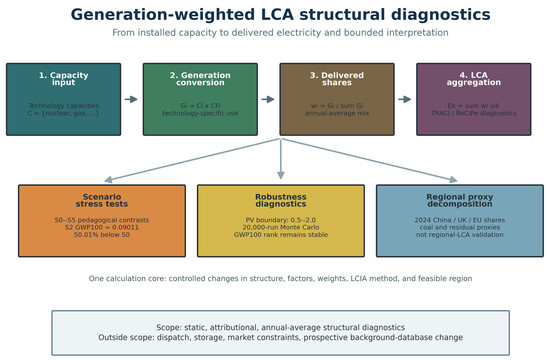
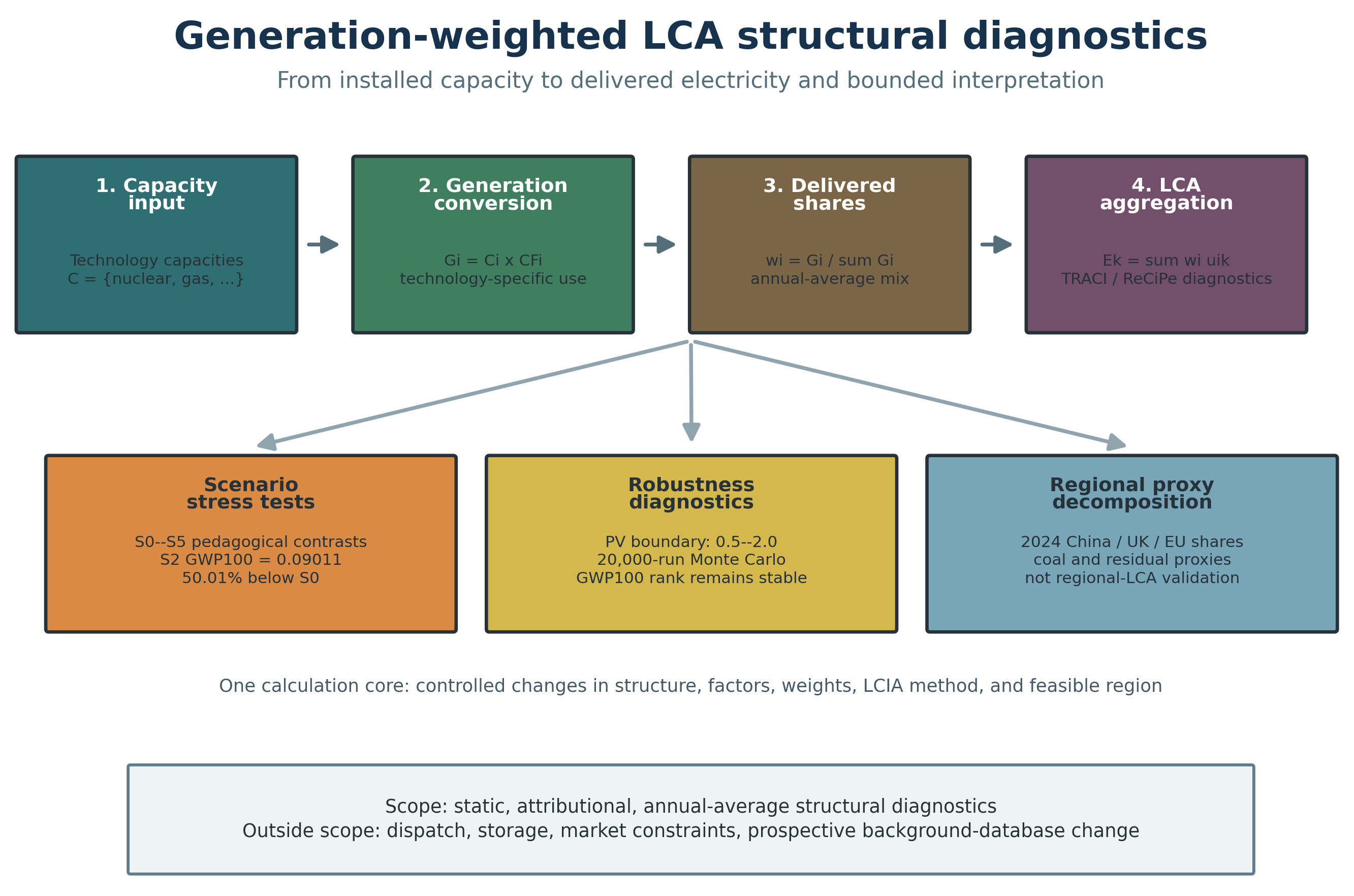
The proposed framework is a deterministic attributional LCA model with uncertainty and boundary-diagnostic extensions. Its computational core is a linear mixing model that maps a technology vector to a vector of environmental indicators. Four linked modules are implemented. Module 1 converts installed-capacity vectors into delivered-generation shares using technology-specific capacity factors. Module 2 multiplies these shares by technology unit-impact vectors and produces scenario-level indicator results. Module 3 evaluates robustness through equal-weight and entropy-weight composite scores, a range of alternative weights, LCIA-method substitution, one-at-a-time parameter perturbation, and Monte Carlo sampling. Module 4 reuses the same linear core for constrained optimization-boundary diagnostics and proxy-based regional generation-mix decomposition. The framework is intentionally static and annual-average; temporal or dynamic LCA requires time-indexed generation and background inventories that are outside the present implementation.

The workflow keeps model inputs, transformations, outputs, and interpretation boundaries explicit, as shown in

Table 1. Model components, implementation, and reusable role.

Element	Implementation in This Study	Reusable Modelling Role
Inputs	Fixed capacity-factor table, scenario capacities, ecoinvent-derived unit-impact matrix, regional generation shares, and proxy-factor tables	Replaceable parameter layer for another electricity mix, region, or LCIA method
State variables	Installed capacities $C_{s,i}$, generation shares $w_{s,i}$, normalized burdens $E_{s,k}/E_{\mathrm{S}0,k}$, and optimized shares $g_i$	Keeps scenario, uncertainty, optimization, and regional proxy states explicit
Transformations	Capacity-to-generation conversion, weighted aggregation, normalization, entropy weighting, Monte Carlo sampling, and linear-program boundary sweeps	Shared computational core for scenario and boundary diagnostics
Outputs	Scenario impacts, rank order, rank probabilities, active constraints, and contribution decompositions	Comparable diagnostics for interpretation and reporting
Diagnostics	One-at-a-time sensitivity, PV-boundary perturbation, ReCiPe substitution, optimization-boundary sweep, and residual-proxy completion	Separates stable findings from method- or boundary-dependent results
Assumptions	Annual-average, attributional, static background inventories, fixed unit-impact vectors, and no dispatch, storage, or market effects	Defines the boundary of inference and the conditions for model transfer

. Capacity, capacity-factor, technology-mapping, unit-impact, residual-proxy, and regional-generation tables are treated as fixed input objects. Intermediate outputs include generation shares, indicator matrices, normalized burdens, rank probabilities, active-constraint frequencies, and contribution decompositions. Final outputs are interpreted as static structural diagnostics rather than dispatch, market, or planning forecasts. The scripts supplied with this manuscript reproduce the scenario calculations, uncertainty tests, optimization-boundary sweeps, and figures from the same input tables.

2.2. Model Scope, Functional Unit, and System Boundary

The functional unit is 1 kWh of electricity output at the process reference-product level (

Table 2. Functional unit and system-boundary definition.

Item	Setting in This Study
Functional unit	1 kWh of electricity output at the process reference-product level
Reference flow	Unit electricity product of the generation-technology inventory; most processes represent high-voltage electricity, while utility-scale ground-mounted PV represents low-voltage electricity and is tested through a separate boundary perturbation
Geographic background	S0–S8 use UK ecoinvent 3.9.1 Cutoff system processes; the regional proxy analysis changes generation shares and applies a China coal proxy only
Included processes	Upstream supply, infrastructure, operational emissions, and end-of-life processes embedded in the selected ecoinvent system processes
Excluded processes	Transmission and distribution losses, storage losses, reserve capacity, dispatch constraints, import adjustments, and market constraints
CHP treatment	Product definitions and allocation follow the corresponding ecoinvent activities
Result type	Annual-average, attributional, static structural diagnostics

). The ecoinvent 3.9.1 database structure and modelling principles follow Wernet et al. [13]; Cutoff allocation and data-quality treatment follow the ecoinvent 3 methodological guidance [25]. For S0–S8, this study uses UK system-process inventory results under the Cutoff allocation model. The selected activities, UUIDs, locations, reference products, voltage levels, and unit-impact values are listed in Supplementary Tables S2 and S3. The built-in boundaries of the selected system processes include upstream fuel supply, infrastructure, operational emissions, and end-of-life treatment as represented in the background database. The model does not add transmission and distribution losses, storage losses, reserve capacity, dispatch constraints, electricity imports, or market constraints. Combined heat-and-power processes retain the product definitions and allocation treatments embedded in the ecoinvent activities.

The main LCIA method is TRACI v2.1, represented by nine indicators: acidification potential (AP), global warming potential over 100 years (GWP100), freshwater ecotoxicity (ECFW), eutrophication potential (EP), human toxicity cancer (HTC), human toxicity non-cancer (HTNC), ozone depletion potential (ODP), particulate matter formation potential (PMFP), and photochemical ozone formation potential using maximum incremental reactivity factors (MIR) [12]. MIR is used as an internal abbreviation for the photochemical ozone formation category and is not treated as a category outside photochemical ozone formation.

Eleven electricity-generation technologies are included: two nuclear processes, four natural-gas processes, hydropower, deep geothermal, onshore wind, offshore wind, and utility-scale solar PV, as shown in

Table 3. Generation technologies and capacity factors.

Group	Technology Code	Description	CF
Nuclear	BWR	Boiling-water-reactor nuclear power	0.723
Nuclear	PWR	Pressurized-water-reactor nuclear power	0.723
Natural gas	NG_CCPP	Natural-gas combined-cycle power plant	0.2775
Natural gas	NG_conv	Conventional natural-gas power generation	0.150
Natural gas	NG_cogen_conv	Conventional gas-fired cogeneration	0.550
Natural gas	NG_cogen_cc	Combined-cycle gas-fired cogeneration	0.600
Renewable	Hydro	Run-of-river hydropower	0.446
Renewable	DGE	Deep geothermal electricity	0.750
Renewable	Wind	Onshore wind power	0.257
Renewable	Wind_offshore	Offshore wind power	0.387
Renewable	Solar_PV_utility	Utility-scale ground-mounted PV	0.098

. Except for utility-scale PV, most reference products are 1 kWh of high-voltage electricity. The UK 570 kWp ground-mounted PV process represents 1 kWh of low-voltage electricity. We do not claim that a $\pm 20\%$ multiplier reconstructs a high-voltage PV inventory; it is a bounded stress test of the voltage and reference-product difference. The selected PV boundary is retained explicitly, and its effect is reported separately. Capacity factors for nuclear power are taken from official UK DUKES statistics [26]. Capacity factors for onshore wind, offshore wind, hydropower, and PV use UK renewable-energy statistics or rounded values derived from them [27]. For gas technologies, exact UK observations aligned with the ecoinvent activities are not available, so operating characteristics are proxied from electricity and district-heating technology data [28]. Deep geothermal uses a global baseload geothermal technology reference [29]. These proxy parameters are included in the sensitivity analysis.

2.3. Capacity-to-Generation Transformation and S0–S5 Scenario Design

For scenario s, let $C_{s,i}$ be the installed capacity of technology i, and let ${\mathrm{CF}}_i$ be its capacity factor. The relative annual generation of technology i is

$$G_{s,i}=C_{s,i}{\mathrm{CF}}_i.$$

(1)

The generation-weighted share is

$$w_{s,i}={\displaystyle \frac{C_{s,i}{\mathrm{CF}}_i}{{\sum }_j{C}_{s,j}{\mathrm{CF}}_j}}.$$

(2)

For environmental indicator k, the per-kWh impact of scenario s is

$$E_{s,k}=\sum _i{w}_{s,i}{u}_{i,k},$$

(3)

where $u_{i,k}$ is the unit environmental impact of technology i for indicator k. The common 8760 h factor cancels during normalization. To compare equal electricity output, total installed capacity can also be scaled so that each scenario gives the same annual generation as S0; this scaling does not change per-kWh generation shares or per-kWh impacts.

S0–S5 are normative stress-test scenarios for comparing technology pathways rather than official UK electricity mixes, forecasts, or grid-scale planning cases. The directions of wind and solar expansion and of nuclear and gas adjustment in S1–S5 are informed by UK decarbonization pathway studies [30,31,32], but those sources do not determine the numerical capacities. The total model scale of 6935 MW is inherited from the lcpy Simple LCA example by Gkousis and Katsou [15]. The original 9-dimensional capacity vector contains an aggregate wind variable, Wind_1_3, with 980 MW. In S0–S5, this variable is split into onshore wind, offshore wind, and utility-scale PV. S0 is an expanded reference case; S1–S5 change four group-level levers while preserving 6935 MW total capacity: nuclear capacity, the four-technology gas capacity pool, hydropower plus deep-geothermal capacity, and the split variable-renewable pool. The resulting group totals are (nuclear, gas, hydro/geothermal, variable renewable) = (2300, 3150, 505, 980) MW for S0, (2300, 1890, 800, 1945) MW for S1, (2427, 1390, 900, 2218) MW for S2, (3120, 2287, 518, 1010) MW for S3, (2427, 2081, 825, 1602) MW for S4, and (2081, 1734, 650, 2470) MW for S5. Within each group, capacities are assigned using the transparent rules in Supplementary Table S1a–c; rounding is absorbed by the final gas component so that every scenario sums to 6935 MW. These six cases were selected to span a reference, high-renewable, low-fossil, high-nuclear, balanced, and wind-led contrast while keeping the technology set and model scale fixed (

Table 4. S0–S5 scenario design and variable renewable-capacity pool.

Scenario	Design Meaning	Original Wind Pool/MW	Onshore Wind/MW	Offshore Wind/MW	PV/MW
S0	Expanded reference	980	330	500	150
S1	High renewable energy	1945	650	950	345
S2	Low fossil energy	2218	700	1100	418
S3	High nuclear power	1010	350	500	160
S4	Balanced transition	1602	500	800	302
S5	Wind-dominated pathway	2470	650	1500	320

). They are therefore pedagogical stress tests, not an exhaustive or statistically representative scenario ensemble. Their rank order is illustrative of these controlled inputs and should not be transferred directly to an actual electricity system.

2.4. Multi-Indicator Scoring and Robustness Diagnostics

The nine TRACI indicators have different units and magnitudes and cannot be summed directly. Each scenario result is first normalized by S0, $x_{s,k}=E_{s,k}/E_{\mathrm{S}0,k}$. Because all nine indicators are burden-type indicators, lower values indicate lower relative burden. The equal-weight composite score is

$${\mathrm{Score}}_s={\displaystyle \frac{1}{9}}\sum _k{\displaystyle \frac{E_{s,k}}{E_{\mathrm{S}0,k}}}.$$

(4)

Entropy weighting is then used as a data-driven check on the equal-weight assumption. After transforming the normalized burden values into positive dimensionless values, the proportion $p_{s,k}$, entropy $e_k$, difference coefficient $d_k$, and weight ${\omega }_k$ are calculated. Because these weights are estimated from only six constructed scenarios, they measure dispersion within this scenario set rather than environmental importance or stakeholder preference. We therefore also vary the GWP100 weight from 0.10 to 0.75 while distributing the remaining weight equally across the other eight indicators. The entropy-weight composite burden remains a weighted sum of negative indicators:

$${\mathrm{Score}}_s^{\mathrm{EW}}=\sum _k{\omega }_k{\displaystyle \frac{E_{s,k}}{E_{\mathrm{S}0,k}}}.$$

(5)

LCIA-method sensitivity is evaluated by replacing TRACI v2.1 with ReCiPe 2016 v1.03 midpoint(H), while keeping the same S0–S5 technology set, capacities, and generation weights [23]. The ReCiPe comparison includes 12 midpoint categories: climate change, terrestrial acidification, freshwater eutrophication, freshwater ecotoxicity, human toxicity (carcinogenic and non-carcinogenic), ozone depletion, particulate matter formation, photochemical ozone formation, ionizing radiation, land use, and water consumption. ReCiPe scores are used only as a sensitivity diagnostic and do not replace the TRACI-based main results.

To address the dependence of optimization on the LCIA method, a parallel ReCiPe midpoint(H) optimization is also solved under the same S6–S7 feasibility constraints. The ReCiPe GWP100 objective minimizes the ReCiPe climate-change category, while the ReCiPe composite objective normalizes all 12 midpoint categories to the ReCiPe S0 result and assigns equal weights. These are method-sensitivity diagnostics rather than additional planning cases; the main optimization remains TRACI-based because the nine TRACI categories define the primary decision criterion of this study.

Deterministic sensitivity tests include two parts. First, each of the 11 capacity factors is perturbed one at a time by $\pm 20\%$. Second, all PV unit impacts are multiplied by 0.8 and 1.2 to test the boundary difference between the low-voltage PV process and the high-voltage processes; an expanded PV stress test uses multipliers from 0.5 to 2.0. The Monte Carlo analysis samples the 11 capacity factors from triangular distributions with the baseline as the mode and $\pm 20\%$ as the bounds and samples the PV multiplier from a uniform distribution over 0.8–1.2. The triangular form places most mass near the stated engineering baseline without treating the bounds as a confidence interval. Each iteration evaluates all six S0–S5 scenarios under the same sampled background. The archived primary analysis uses 1000 iterations, giving 6000 scenario outcomes; a 20,000-iteration convergence and correlation stress test is reported in Supplementary Table S5. The correlation stress test uses Gaussian-copula dependence with within-group correlation $\rho =0.5$ for nuclear, gas, and renewable groups. Technology-impact correlations are not sampled because no covariance matrix is available in the licensed inventory export; this is a remaining uncertainty limitation.

2.5. Constrained Optimization-Boundary Diagnostics

After the S0–S5 scenario assessment, S6–S8 are constructed as constrained optimization-boundary diagnostics rather than additional planning scenarios. The optimization is solved in generation-share space, using the same 11 technology categories as the scenario model. Let $g_i$ denote the generation-share decision variable for technology i. The corresponding capacity share, reported only for interpretation, is back-calculated as

$$c_i={\displaystyle \frac{g_i/{\mathrm{CF}}_i}{{\sum }_j{g}_j/{\mathrm{CF}}_j}}.$$

(6)

The objective is therefore linear in the variables used by the solver. If the same problem is rewritten directly in installed-capacity variables, the objective becomes linear-fractional because generation shares are normalized by total capacity-factor-weighted generation. S6 minimizes ${\sum }_i{g}_i{u}_{i,\mathrm{GWP}100}$. S7 minimizes the equal-weight normalized composite objective $(1/9){\sum }_k[{\sum }_i{g}_i{u}_{i,k}/E_{\mathrm{S}0,k}]$. S8 raises the minimum renewable-generation share to test a single-boundary response.

Table 5. S6–S8 decision variables and boundary thresholds.

Element	Implementation in the Linear Program	Threshold or Setting
Decision variables	Generation-share variables for BWR, PWR, NG_CCPP, NG_conv, NG_cogen_conv, NG_cogen_cc, Hydro, DGE, Wind, Wind_offshore, and Solar_PV_utility	$0\le g_i\le 1$, ${\sum }_i{g}_i=1$
Nuclear boundary	$g_{\mathrm{BWR}}+g_{\mathrm{PWR}}$	≤0.45
Fossil boundary	Sum of the four natural-gas generation shares	≤0.30 in S6/S7; ≤0.40 in the S8 sweep
Renewable boundary	Hydro + DGE + Wind + Wind_offshore + Solar_PV_utility	≥0.40 in S6/S7; 0.30–0.60 in S8
Wind boundary	Wind + Wind_offshore	≤0.60
Solar boundary	Solar_PV_utility	≤0.30
Hydro boundary	Hydro	≤0.20
DGE boundary	DGE	≤0.10

lists the S6–S8 decision variables and boundary thresholds. The implementation uses scipy.optimize.linprog (SciPy v1.17.1) with the HiGHS backend (https://highs.dev, accessed on 2 August 2026). A multi-boundary sensitivity test varies seven boundary classes simultaneously, creating 3456 boundary combinations; each is solved for both GWP100 minimization and composite-score minimization, for 6912 optimizations. A constraint is counted as active when its slack is no greater than ${10}^{-6}$. This step reveals boundary dependence in the feasible region.

2.6. Verification, Reproducibility, and Interpretation Controls

Three controls make the modelling results auditable. First, internal arithmetic checks verify that all generation-share vectors sum to one after capacity-to-generation conversion and that the common 8760 h factor cancels in the normalized per-kWh calculation. Second, scenario ranking robustness is tested by changing parameters, weights, and LCIA method while holding the scenario definitions fixed. Third, the regional proxy module is reported in staged cases—core-six, China-coal-proxy, and residual-proxy completion—so that changes caused by generation structure can be separated from changes caused by proxy factors.

The reproducibility package contains the Python 3.12.13 scripts, figure-generation scripts, dependency list, and reproduction notes. Randomness is restricted to the Monte Carlo module, where the number of iterations, parameter ranges, distribution forms, and the seed are stored with the analysis scripts. The reproduction notes also document the two reproduction levels: a full raw-inventory rebuild requiring a licensed ecoinvent 3.9.1 JSON-LD export and lcpy(v1.0.0)/Brightway(bw2data 4.7, bw2calc 2.4.0) environment, and a downstream reproduction route that starts from fixed numerical output tables and regenerates the reported figures. No statistical model is fitted to the regional observations, but capacity factors, the PV multiplier, and residual-category coefficients are still modelling choices rather than known constants. They are therefore subjected to explicit sensitivity checks and are not described as calibrated regional inventories. The regional proxy exercise is a mathematical and structural diagnostic of the weighted-sum calculation, not validation of a fully regionalized electricity LCA inventory. As an external factor check, the headline GWP100 results are additionally recomputed with IPCC AR5 [33] and UNECE 2021 [1] literature factor sets under fixed capacities, capacity factors, and mapping rules, together with a 20,000-draw uniform-range stress test and an exact 256-vertex endpoint enumeration (Supplementary Materials S11).

2.7. UK Observational Backcast

The capacity-to-generation transformation is evaluated against official UK observations rather than only against the synthetic S0–S5 scenarios. Annual generation and gas/nuclear capacity are taken from Tables 5.6 and 5.7 of the DUKES 2025 publication [26], while actual nameplate capacity and generation for natural-flow hydropower, onshore wind, offshore wind, and solar PV are taken from Table 6.2 of the DUKES publication [34]. DUKES Table 5.7 de-rates wind, solar, and small-scale hydro capacity and is therefore not used for those technologies [26]. The six directly matched categories cover 81.2–83.9% of UK gross generation during the 2020–2024 backcast period.

Because capacity can change during a calendar year, annual generation is paired with mean capacity,

$${\overline{C}}_{t,i}={\displaystyle \frac{C_{t-1,i}+C_{t,i}}{2}}.$$

(7)

Three estimators are compared. The capacity-only estimator normalizes ${\overline{C}}_{t,i}$. The fixed-factor estimator normalizes ${\overline{C}}_{t,i}{\mathrm{CF}}_i^{2024}$, using the manuscript capacity factors and the official 2024 CCGT factor for the aggregate DUKES gas category. The dynamic comparator normalizes ${\overline{C}}_{t,i}{\mathrm{CF}}_{t-1,i}^{\mathrm{obs}}$, so that only information available in the preceding year is used. Observed shares normalize actual annual generation. Performance is measured using technology-share mean absolute error (MAE), root-mean-square error, Jensen–Shannon distance, and GWP100 error under the same unit-impact factors. Uncertainty in the MAE improvement is estimated by 20,000 year-level bootstrap resamples with seed 20260804. The exact paired one-sided sign test is retained only as a descriptive count of year-level wins; with five years it has low statistical power and is not treated as independent validation evidence. This is an observational backcast of the weighting module, not a fitted dispatch model.

2.8. Regional Generation-Mix Transfer

As a proxy exercise for observed annual electricity structures, the analysis replaces scenario-derived generation weights with 2024 annual generation shares for China, the UK, and the EU. The main statistical source is the Our World in Data electricity-production-by-source dataset, based on Ember yearly electricity data and Energy Institute statistics [35]. The dataset is used only to calculate generation shares; the unit TWh cancels during normalization, so the result remains a per-kWh impact. The OWID/Ember data are cross-checked against official UK DUKES statistics [26], the China Statistical Yearbook 2025 [36], and National Energy Administration power-industry statistics [37,38]. For China, a regional coal proxy uses 31 provincial hard-coal processes weighted by 2022 provincial thermal-power generation reported in the China Electric Power Statistical Yearbook 2024 [39]. Thermal generation includes non-coal sources such as gas, oil, and biomass, so these weights cannot be interpreted as provincial coal-generation shares. Because province-level coal-only generation was not located in a directly reusable public table, this treatment is retained only as a lagged proxy stress test for the coal factor and is not presented as a validated regional coal inventory.

The regional calculation applies Equation (3) with the region index r replacing the scenario index s, where r is region, i is generation technology or statistical electricity-source category, k is environmental indicator, $w_{r,i}$ is the observed annual generation share, and $u_{i,k}$ is the corresponding unit impact factor. The core-six analysis includes coal, gas, nuclear, hydropower, wind, and solar. Coal uses a newly introduced coal factor; gas maps to a natural-gas technology combination or NG_CCPP proxy; nuclear maps to the BWR/PWR combination; hydropower, wind, and solar map to Hydro, Wind/Wind_offshore, and Solar_PV_utility. Residual categories—oil, bioenergy, and other renewables—are tested through low, central, and high internal proxy cases. The core-six version identifies structural effects while leaving full regionalized electricity-inventory construction to future work.

Table 6. Proxy treatments and interpretation boundaries for regional diagnostics.

Treatment	Proxy or Control	Permitted Interpretation
China/UK/EU core-six comparison	Same technology factors for all three regions; generation weights are changed	Identifies structural weighting effects; does not claim a complete regionalized LCA
China coal factor	31 provincial hard-coal processes weighted by provincial thermal generation	Tests coal-factor sensitivity; not a final China coal inventory
Oil, bioenergy, and other renewables	Low, central, and high internal proxy cases	Tests whether omitted categories alter the main inference; not region-specific inventory modeling
China coal proxy timing	2022 provincial thermal-generation weights used as a proxy for the 2024 coal factor	Interpreted as a lagged proxy rather than a 2024 final value
UK and EU absolute values	Higher residual-category shares are reported with proxy uncertainty	Supports comparison of magnitude and direction; fine ranking is not overinterpreted
S6–S8 optimization structures	Capacity is optimized, but results are reported as generation shares	Diagnoses boundary dependence; not a planning prescription

summarizes the proxy treatments and their permitted interpretations.

3. Results

3.1. Scenario-Simulation Output: Capacity-Based Versus Generation-Weighted GWP100

Table 7. Core S0–S5 results under generation weighting.

Scenario	GWP100	Reduction Relative to S0/%	Equal-Weight Score	GWP Rank	Composite Rank
S0	0.18027	0.00	1.0000	6	6
S1	0.11748	34.83	0.9180	3	4
S2	0.09011	50.01	0.8781	1	1
S3	0.12538	30.45	0.8808	5	2
S4	0.12478	30.78	0.9019	4	3
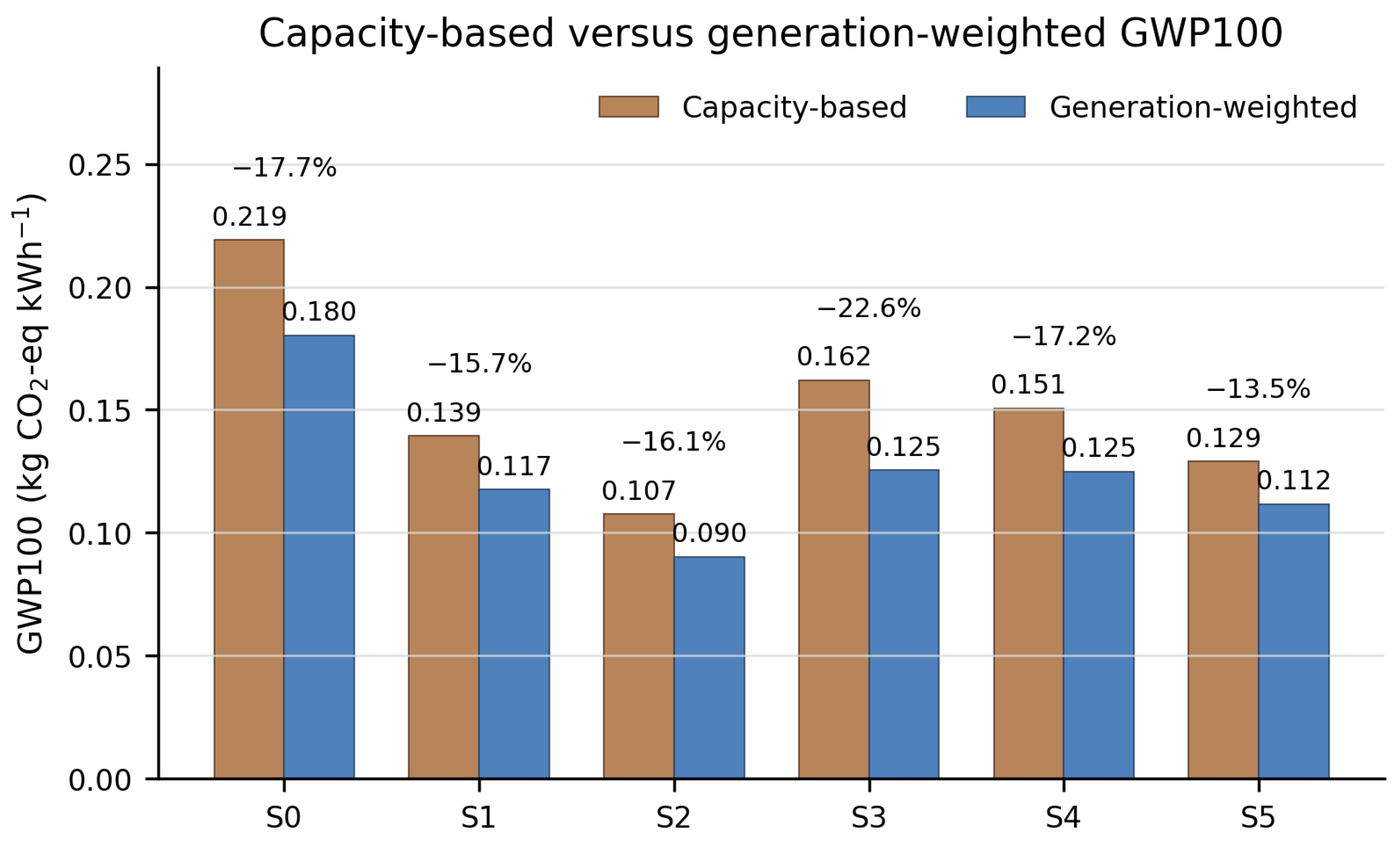
S5	0.11155	38.12	0.9198	2	5

reports the core S0–S5 results under capacity-based and generation-weighted shares. GWP100 is first calculated under capacity-based shares and generation-weighted shares, providing a direct test of generation weighting. Under capacity-based shares, S0–S5 GWP100 values are 0.21904, 0.13932, 0.10742, 0.16197, 0.15062, and 0.12902 kg CO₂-eq kWh⁻¹, respectively. After conversion to generation-weighted shares, the corresponding values fall to 0.18027, 0.11748, 0.09011, 0.12538, 0.12478, and 0.11155 kg CO₂-eq kWh⁻¹, a reduction of 13.55–22.59% relative to the capacity-based calculation. In S0, for example, the BWR nuclear share rises from 21.63% under the capacity-based calculation to 30.25% under the generation-weighted calculation, while conventional natural-gas generation falls from 10.82% to 3.14%. The GWP100 values are reported to five decimal places for traceability and scenario comparison; this does not imply equivalent measurement precision in the underlying inventory or characterization factors.

The generation-weighted GWP100 ranking is S2, S5, S1, S4, S3, and S0, as shown in Figure 1. S2 reaches 0.09011 kg CO₂-eq kWh⁻¹, 50.01% below S0. S5 and S1 reduce GWP100 by 38.12% and 34.83%, respectively. Under the present technology factors and generation weights, lowering the generation share of fossil technologies, especially gas in the S0–S5 technology set, is the main modelled mechanism for climate-change reduction. S3 raises nuclear capacity but retains more gas-fired generation, which explains why its GWP100 reduction is smaller than that of S1, S2, and S5.

3.2. Multi-Indicator Model Output and Entropy-Weighting Response

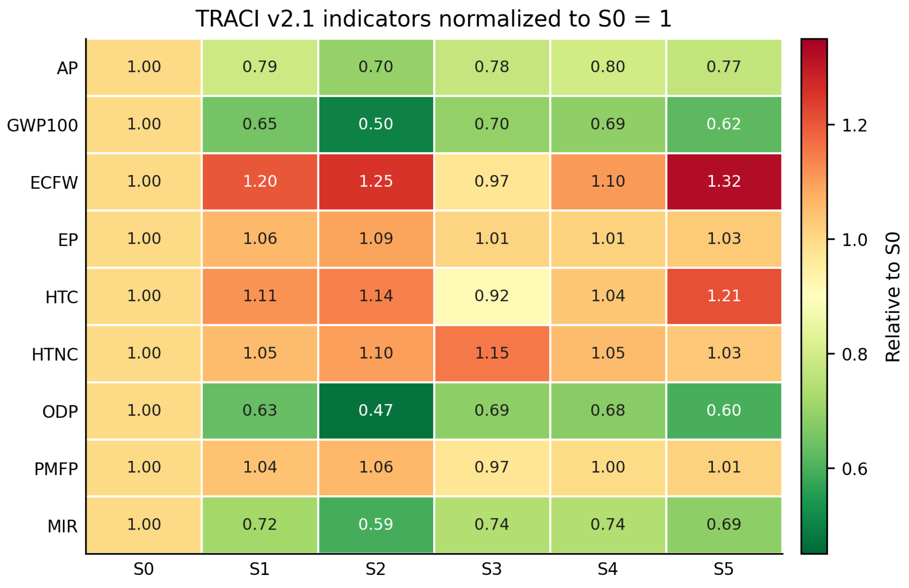
The multi-indicator TRACI results show that the GWP100 ranking cannot be transferred directly to all impact categories. In the equal-weight composite score, S2 and S3 are nearly tied, with scores of 0.8781 and 0.8808; the difference is only 0.00265. S2 has the strongest climate-change reduction, but higher renewable, PV, and geothermal shares raise some toxicity, ecotoxicity, and eutrophication indicators. S3, with a higher nuclear share, performs more evenly for several non-carbon indicators, as shown by the nine normalized TRACI indicators in Figure 2.

Entropy weighting tests whether the equal-weight score is sensitive to the weighting assumption. ECFW, HTC, and PMFP receive entropy weights of 0.1485, 0.1381, and 0.1265, higher than the equal-weight value of 0.1111. GWP100, ODP, MIR, and AP receive weights near 0.09. Under entropy weighting, the scenario order becomes S3, S2, S4, S1, S5, and S0. S2 and S3 switch order, but both remain the top two scenarios; they have closely comparable composite performance, and neither is a unique optimum across weighting schemes. In the explicit GWP100-weight stress test, S2 remains first for GWP100 weights of 0.10, 0.111, 0.25, 0.50, and 0.75, but the runner-up changes from S3 to S5 at the larger weights. The smallest S2–runner-up score gap is only 0.00024 at GWP100 weight 0.10, which reinforces that the robust claim is about the GWP100 rank, not a universal composite optimum.

Table 8. Equal-weight and entropy-weight composite scores.

Scenario	Equal Score	Equal Rank	Entropy Score	Entropy Rank
S0	1.0000	6	1.0000	6
S1	0.9180	4	0.9515	4
S2	0.8781	1	0.9242	2
S3	0.8808	2	0.8971	1
S4	0.9019	3	0.9268	3
S5	0.9198	5	0.9623	5

lists the equal-weight and entropy-weight composite scores and ranks.

3.3. Parameter Sensitivity and Monte Carlo Rank Stability

Table 9. Sensitivity and Monte Carlo result summary.

Analysis	Main Setting	Effect on GWP100	Effect on Composite Ranking
Capacity-factor one-at-a-time sensitivity	Each of 11 technologies perturbed by $\pm 20\%$	S2 rank remains stable; maximum change about 5.96–7.75%	S2 and S3 can switch
PV boundary perturbation	All nine PV indicators multiplied by 0.8 and 1.2	GWP100 ranking unchanged; maximum change below 0.206%	S3 can exceed S2 when PV impacts increase by 20%
Monte Carlo	1000-run archive; 20,000-run convergence and $\rho =0.5$ stress checks	S2 is first in 100% of runs; 20,000-run margin 0.02143 kg CO2-eq kWh−1	S2 is first in 68.2% of independent runs and 66.5% under correlated factors; S3 takes the remainder

summarizes the sensitivity and Monte Carlo results. The one-at-a-time capacity-factor sensitivity analysis shows maximum relative GWP100 changes of about 5.96–7.75% and maximum composite-score changes of about 2.10–2.55%. The GWP100 ranks of S0, S1, S2, and S5 remain stable, while S3 and S4 can switch fourth and fifth place under some perturbations. For composite scores, S2 and S3 can switch the top two positions, confirming that the composite ranking is more sensitive than the climate-change ranking.

Perturbing all PV unit impacts by $\pm 20\%$ has no material effect on the GWP100 ranking; the maximum GWP100 change is below 0.206%, and S2 remains first. An expanded stress test with PV multipliers from 0.5 to 2.0 changes GWP100 by at most 1.03% and still leaves S2 first in every case. When PV unit impacts are increased by 20% or more; however, S3 can exceed S2 in the composite score. The low-voltage PV process boundary therefore does not overturn the low-fossil climate-change result within the tested envelope, but it matters for narrow composite-score differences between S2 and S3.

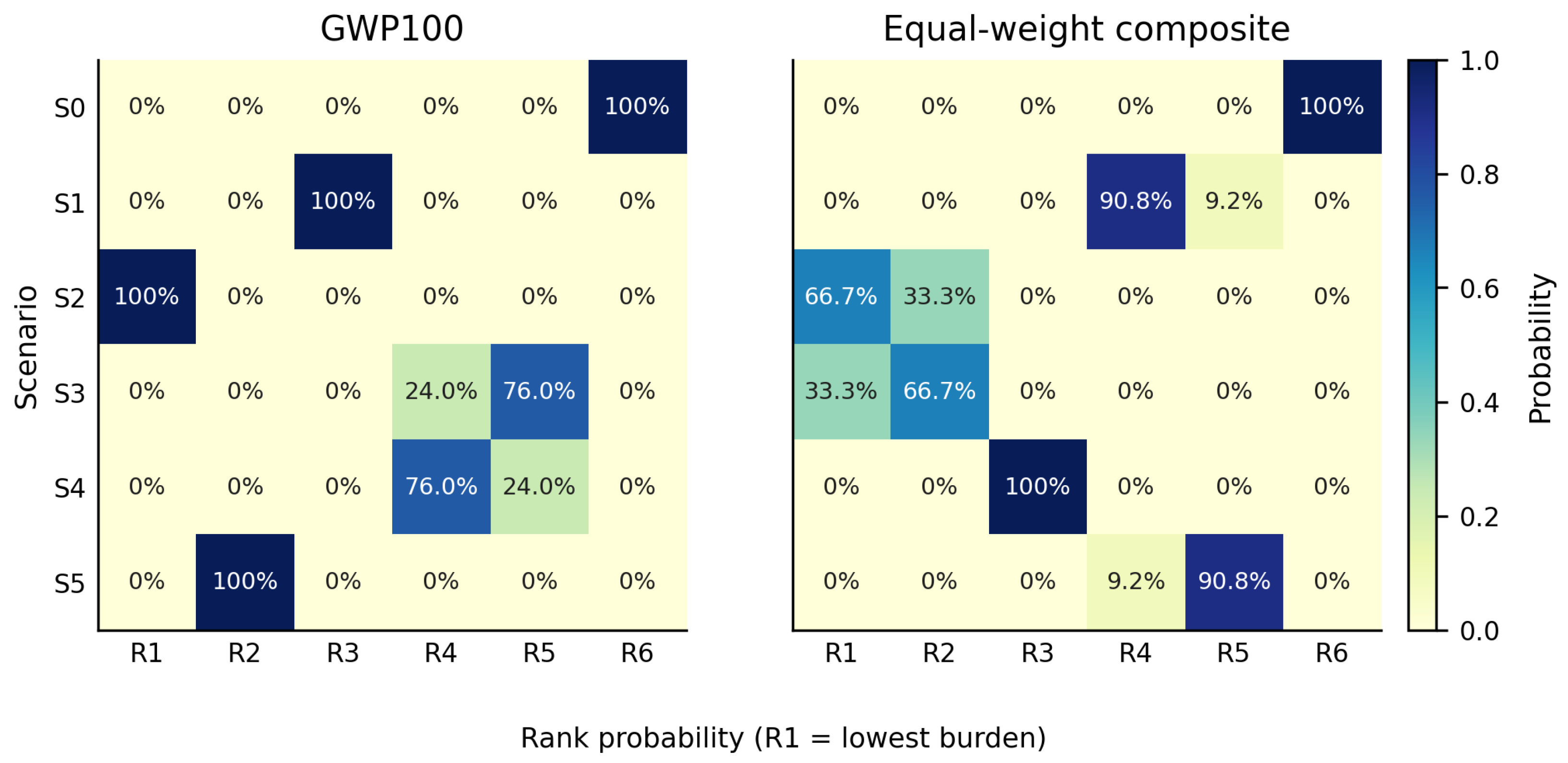
The archived 1000-run Monte Carlo simulation quantifies this difference in stability. For GWP100, S2 ranks first in every run, S5 ranks second in every run, and S0 ranks last in every run, as shown in Figure 3. S3 and S4 exchange the fourth and fifth positions with probabilities of 0.24/0.76 and 0.76/0.24, respectively. The expanded 20,000-run check gives the same GWP100 result: S2 is first in 100% of runs, and its mean advantage over the closest competing scenario is 0.02143 kg CO₂-eq kWh⁻¹ (2.5th–97.5th percentile: 0.01961–0.02329). For the composite score, S2 ranks first with probability 0.682 and second with probability 0.318 in the expanded run; the correlated-factor stress test changes these values to 0.665 and 0.335. S3 has the complementary first/second probabilities, and S4 remains the next low-burden scenario. The climate-change advantage of S2 is therefore stable within the tested parameter ranges, whereas the S2/S3 composite ordering depends on weighting, parameter choices, and dependence assumptions.

3.4. UK Observational Backcast Results

The observational comparison confirms that capacity-factor weighting improves representation of delivered generation, while also defining the limit of a static factor vector. Across 2020–2024, capacity-only shares have a mean technology-share MAE of 0.0533 and a mean Jensen–Shannon distance of 0.1687 (

Table 10. UK 2020–2024 observational backcast summary.

Method	Mean Share MAE	Mean JS Distance	MAE Reduction vs. Capacity	Mean GWP100 APE
Capacity share	0.0533	0.1687	–	5.33%
Fixed 2024 CF	0.0213	0.0515	60.1%	11.69%
Lagged annual CF	0.0148	0.0353	72.3%	8.70%

). Fixed 2024 capacity-factor weighting reduces these values to 0.0213 and 0.0515. The mean MAE reduction is 60.1%, with a year-bootstrap 95% interval of 44.2–76.8%. Using the preceding year’s observed capacity factors further lowers mean MAE to 0.0148 and Jensen–Shannon distance to 0.0353, a 72.3% MAE reduction with a 95% interval of 66.0–78.3%. Both weighted estimators outperform capacity-only shares in every backcast year (5/5; exact paired one-sided sign test $p=0.03125$ for each comparison). Because $n=5$, this sign-test result is reported as an illustrative year-level consistency check with low power, not as standalone validation evidence. Year-by-year technology errors are given in Supplementary Table S6a–c. We did not add a regression benchmark because the target is the deterministic capacity-to-generation mapping rather than fitted dispatch prediction, and the matched annual panel is short. Instead, two zero-fitting historical benchmarks are evaluated over the same backcast windows: naive persistence, which reuses the preceding year’s observed shares, and the expanding arithmetic mean of all preceding annual observed-share vectors. Over 2020–2024, the historical-mean benchmark gives a mean MAE of 0.0363 and naive persistence 0.0169, compared with 0.0213 for the fixed-factor estimator and 0.0148 for the lagged-factor comparator; the lagged comparator also beats naive persistence in seven of nine years over 2016–2024 (Supplementary Table S10a,b). Because the lagged comparator uses target-year average capacity with preceding-year factors, it is retained as a backcast diagnostic rather than a strict ex-ante forecast.

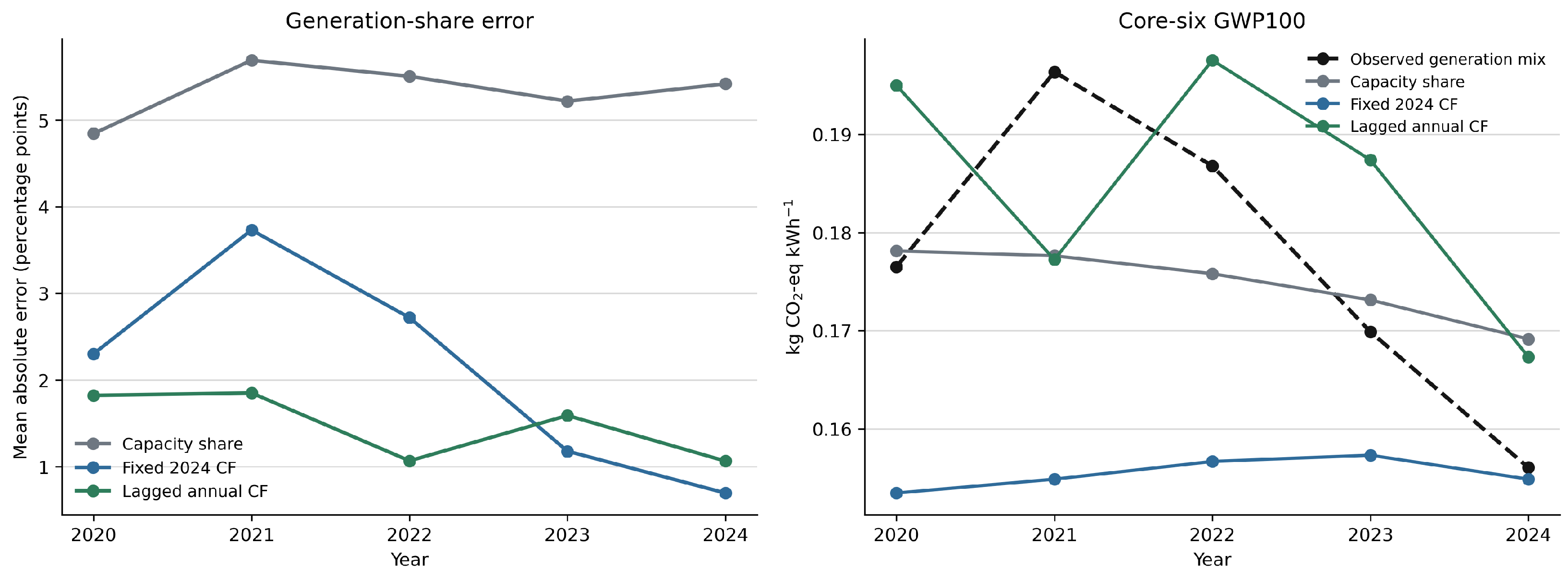
The impact comparison is more nuanced. In 2024, fixed-factor GWP100 is 0.15487 kg CO₂-eq kWh⁻¹, versus 0.15605 for the observed core-six mix, an absolute error of 0.76%; the capacity-only error is 8.39% (Figure 4). Across all five backcast years, however, mean absolute GWP100 percentage error is 5.33% for capacity-only, 11.69% for fixed factors, and 8.70% for lagged annual factors. Capacity-only errors partly cancel in the GWP-weighted sum, whereas fixed factors do not reproduce the sharp interannual change in gas utilization. Generation weighting therefore improves mix fidelity but does not by itself turn a static annual-average model into a temporal predictor. An extended check using the same public data covers 2015–2024 for capacity-only and fixed-factor estimators and 2016–2024 for the lagged estimator, because a preceding-year factor is unavailable for 2015. The fixed-factor mean share MAE was 0.0255 versus 0.0565 for capacity-only, a 54.9% reduction; the lagged estimator gave 0.0149 versus the same 0.0565 baseline, a 73.6% reduction. This longer check supports the direction of the result but also shows why coverage and year-to-year utilization variation should accompany any pooled statistic.

3.5. LCIA-Method Substitution as a Model-Robustness Test

Table 11. Core LCIA-method sensitivity results.

Scenario	ReCiPe Score	ReCiPe Rank	ReCiPe GWP100	ReCiPe GWP Rank	TRACI Score Rank	TRACI GWP Rank
S3	0.9326	1	0.12800	5	2	5
S4	0.9494	2	0.12742	4	3	4
S2	0.9544	3	0.09209	1	1	1
S5	0.9601	4	0.11394	2	5	2
S1	0.9695	5	0.11999	3	4	3
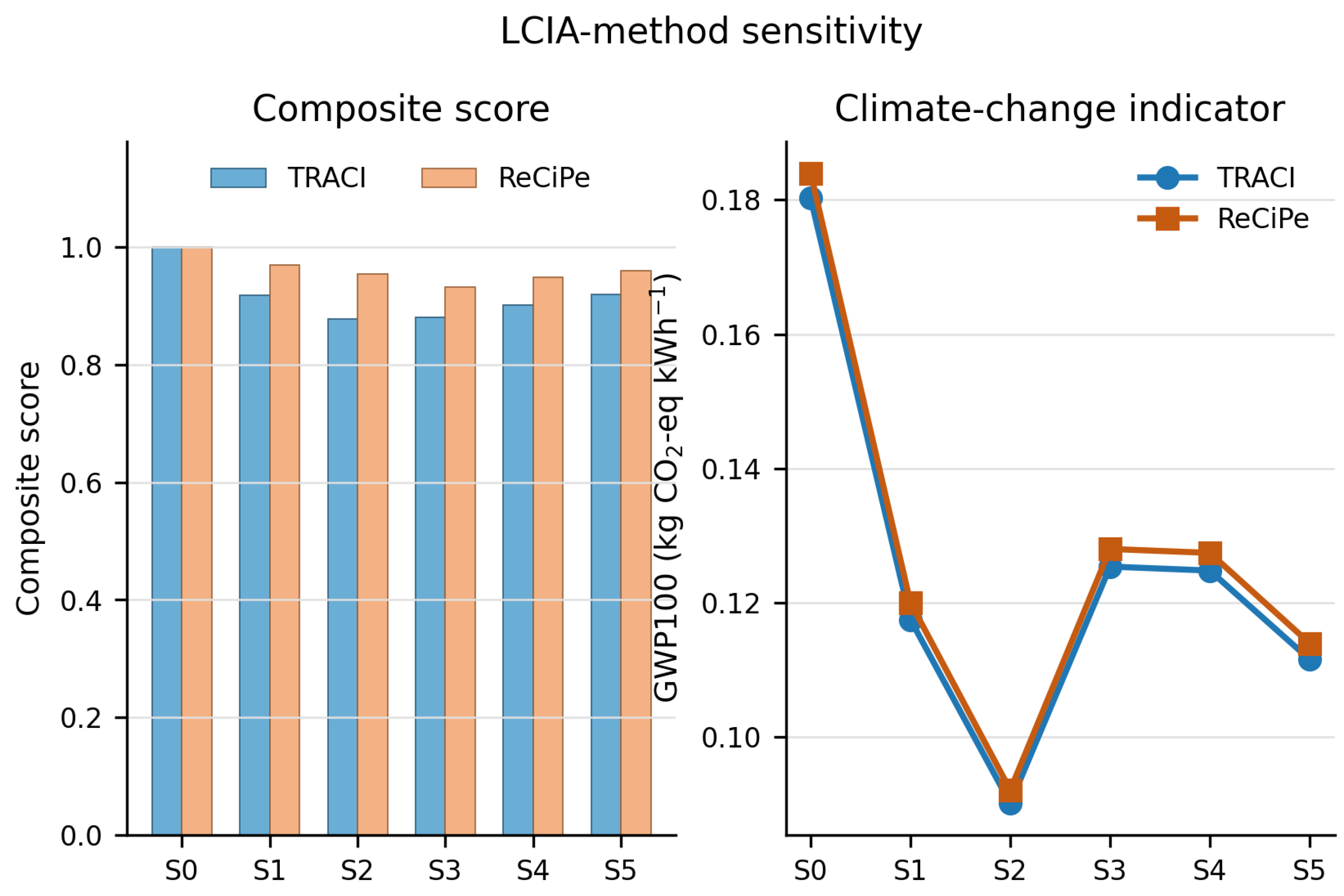
S0	1.0000	6	0.18398	6	6	6

reports the core LCIA-method sensitivity results. Replacing TRACI v2.1 with ReCiPe 2016 midpoint(H) leaves the GWP100 interpretation essentially unchanged. Under ReCiPe GWP100, S2 remains the lowest-impact scenario, with 0.09209 kg CO₂-eq kWh⁻¹; S5 and S1 rank second and third, and S0 remains highest. The climate-change inference—lowering fossil generation shares reduces GWP100—thus does not depend on TRACI alone.

The multi-indicator score is more method-dependent. Under ReCiPe equal weighting, the order is S3, S4, S2, S5, S1, and S0, compared with the TRACI equal-weight order S2, S3, S4, S1, S5, and S0, as shown in Figure 5. The difference arises partly because ReCiPe includes categories not covered in the TRACI main analysis, such as ionizing radiation, land use, and water consumption, and partly because characterization models differ for toxicity, particulate matter, and photochemical ozone formation. S2, S3, and S4 therefore form a low-burden group for multi-indicator assessment, while the exact order varies with method and indicator set.

3.6. Optimization-Boundary Response and Active Constraints

S6–S8 differ from S0–S5 in purpose. They are constrained optimization diagnostics on the split technology set, not predesigned normative scenarios.

Table 12. S6–S8 and multi-boundary sensitivity results.

Item	Result
S6 GWP100 minimization	Model response: PWR 45%, Hydro 20%, wind/PV group 35%
S7 composite-objective minimization	Same response as S6
S8 RES 30–50%	Same response as S6/S7
S8 RES 60%	PWR 40%, Hydro 20%, wind/PV group 40%
ReCiPe GWP100 diagnostic	PWR 45%, Hydro 20%, onshore wind 35%; ReCiPe GWP100 $=0.00882$
ReCiPe composite diagnostic	PWR 45%, Hydro 20%, offshore wind 35%; ReCiPe GWP100 $=0.00975$
Multi-boundary sensitivity scale	3456 boundary combinations × 2 objectives = 6912 optimizations
Active constraints	Hydro 100%, nuclear 87.5%, wind/PV group 27.6%
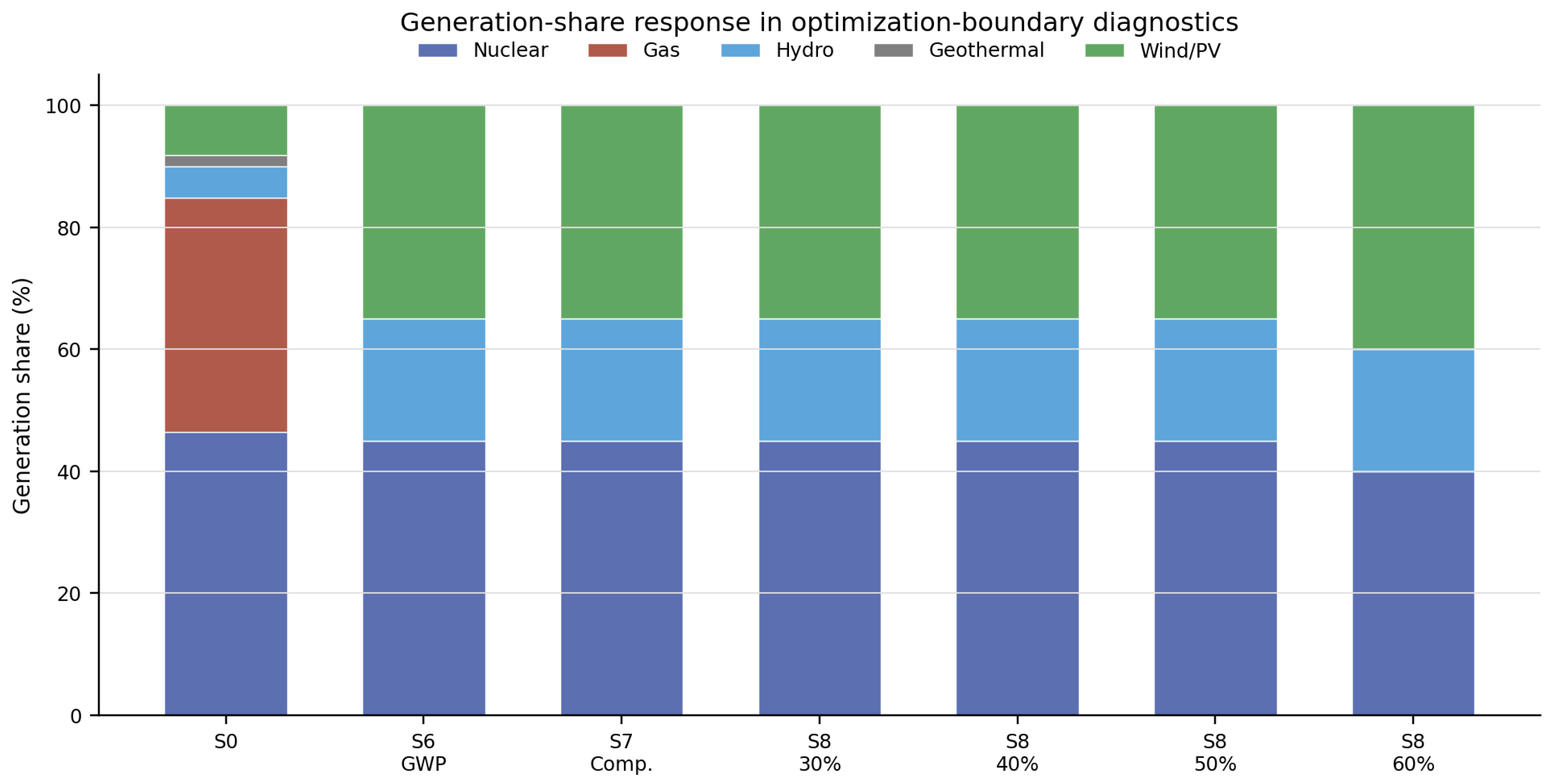
Interpretation boundary	Boundary-dependence diagnostic, not a deployable planning mix

summarizes the S6–S8 outcomes and the multi-boundary sensitivity results. Under the given constraints, S6 GWP100 minimization and S7 equal-weight composite minimization both return the same generation-share response: PWR 45%, run-of-river hydropower 20%, and the wind/PV group 35%, as shown in Figure 6. The corresponding GWP100 is 0.00852 kg CO₂-eq kWh⁻¹. When the renewable-generation lower bound in S8 is set between 30% and 50%, the same response is obtained. When the renewable lower bound is raised to 60%, the response becomes PWR 40%, hydropower 20%, and the wind/PV group 40%, with GWP100 increasing to 0.00886 kg CO₂-eq kWh⁻¹.

The parallel ReCiPe optimization makes the method dependence explicit. Under the same constraints, ReCiPe GWP100 minimization selects PWR 45%, hydropower 20%, and onshore wind 35%, with ReCiPe GWP100 of 0.00882 kg CO₂-eq kWh⁻¹. ReCiPe equal-weight composite minimization selects PWR 45%, hydropower 20%, and offshore wind 35%, with ReCiPe GWP100 of 0.00975 kg CO₂-eq kWh⁻¹. The shared nuclear and hydropower bounds but different wind subtype indicate that the optimization result is method- and constraint-dependent rather than a universal technology prescription.

In this constrained problem, the model preferentially selects PWR, hydropower, and the wind/PV group under the current unit impact factors and bounds. In the multi-boundary sensitivity analysis, the hydropower upper bound is active in 100% of solutions for both optimization objectives. The nuclear upper bound is active in 87.5% of solutions, the wind upper bound in about 27.6%, and the renewable lower bound in about 25.0–28.6%. The fossil upper bound and solar upper bound are not active within the tested range. Any claim about an environmentally optimal electricity structure should therefore report the source of constraints and the sensitivity of the optimum to those constraints.

3.7. Regional Proxy Simulation and Contribution Decomposition

The same calculation core can be written as a weighted sum of technology unit impacts and generation shares. In S0–S5, generation shares come from normative capacity scenarios and capacity factors. In S6–S8, they come from constrained optimization. In this section, they are replaced by observed 2024 annual generation shares for China, the UK, and the EU. This is a mathematical substitution and structural decomposition under a common factor system, not an external validation of regional LCA results, because most unit-impact factors remain UK-background or internally proxied factors.

The core-six coverage is high for China and the EU and lower for the UK because UK bioenergy is a larger residual category. In 2024, coal supplied 57.77% of China’s electricity, compared with 0.67% in the UK and 9.77% in the EU. Fossil generation accounted for 61.83% of China’s electricity, while nuclear, hydro, wind, and solar together accounted for 36.10%. The corresponding nuclear-hydro-wind-solar shares were 50.82% for the UK and 65.54% for the EU. The core-six categories cover 97.05%, 81.86%, and 90.89% of generation in China, the UK, and the EU, respectively (

Table 13. Real generation structures and core-six coverage for 2024.

Region	Total/TWh	Coal/%	Fossil/%	Nuclear/Hydro/Wind/Solar/%	Core-Six Coverage/%
China	10086.88	57.77	61.83	36.10	97.05
UK	284.16	0.67	35.07	50.82	81.86
EU27	2773.21	9.77	28.57	65.54	90.89

).

Two calculation cases distinguish generation-structure effects from the coal-factor proxy (

Table 14. Core-six GWP100 under common-factor and China-coal-proxy cases.

Calculation Case	China	UK	EU27	Diagnostic Purpose
Common UK background factors	0.6469	0.1883	0.2051	Identifies generation-share effects
China coal regional proxy	0.7603	0.1883	0.2051	Tests the influence of the China coal proxy

). In the common-UK-background case, all three regions use the same technology factors, so the comparison isolates changes in generation shares. In the regionalized-coal-proxy case, only China’s coal factor is replaced by the provincial hard-coal proxy; all other technology factors remain unchanged. Under the common-factor case, core-six GWP100 values are 0.6469, 0.1883, and 0.2051 kg CO₂-eq kWh⁻¹ for China, the UK, and the EU, respectively. Replacing only the China coal factor raises China’s result to 0.7603 kg CO₂-eq kWh⁻¹, a 17.53% proxy-induced increase, while the UK and EU values remain unchanged. Because the weighting basis is thermal rather than coal-only, this increase cannot be interpreted as a measured regional coal-supply effect. A weighting-basis stress test using national coal and gas generation anchors [39] and literature-informed gas-cluster allocations [40] changes the increase only from 17.53% to 18.46% across the tested concentration cases, and capacity-constrained fixed-mass bounds delimit 11.89–20.38% (Supplementary Table S9). Sequential decomposition indicates that the structural effect explains about 80.17% of the China–UK GWP100 gap and 79.57% of the China–EU gap; the coal-proxy substitution contributes the remaining 19.83% and 20.43%. This is a diagnostic decomposition within the model boundary, not causal attribution or regional validation. Under the literature-factor substitution, China remains the highest of the three regions in all five literature factor sets, in all 20,000 uniform-range draws, and at all 256 endpoint vertices, whereas the UK–EU fine ranking reverses under some factor sets and is therefore not overinterpreted (Supplementary Table S11c,d).

Contribution analysis explains the structural effect. Under the China-coal-proxy case, coal contributes 96.84% of China’s core-six GWP100. In the UK, coal contributes only 4.54%, and gas contributes 89.20%. In the EU, coal and gas contribute 54.84% and 37.85%, respectively. The China coal-proxy GWP100 factor is 1.2368 kg CO₂-eq kWh⁻¹, 18.21% higher than the UK coal factor of 1.0462 kg CO₂-eq kWh⁻¹. The common-factor case shows, however, that China remains highest even without this higher coal-proxy value. The dominant structural contributor to China’s modeled GWP100 is the coal generation share, while the magnitude of the coal-factor difference remains conditional on the thermal-generation weighting proxy.

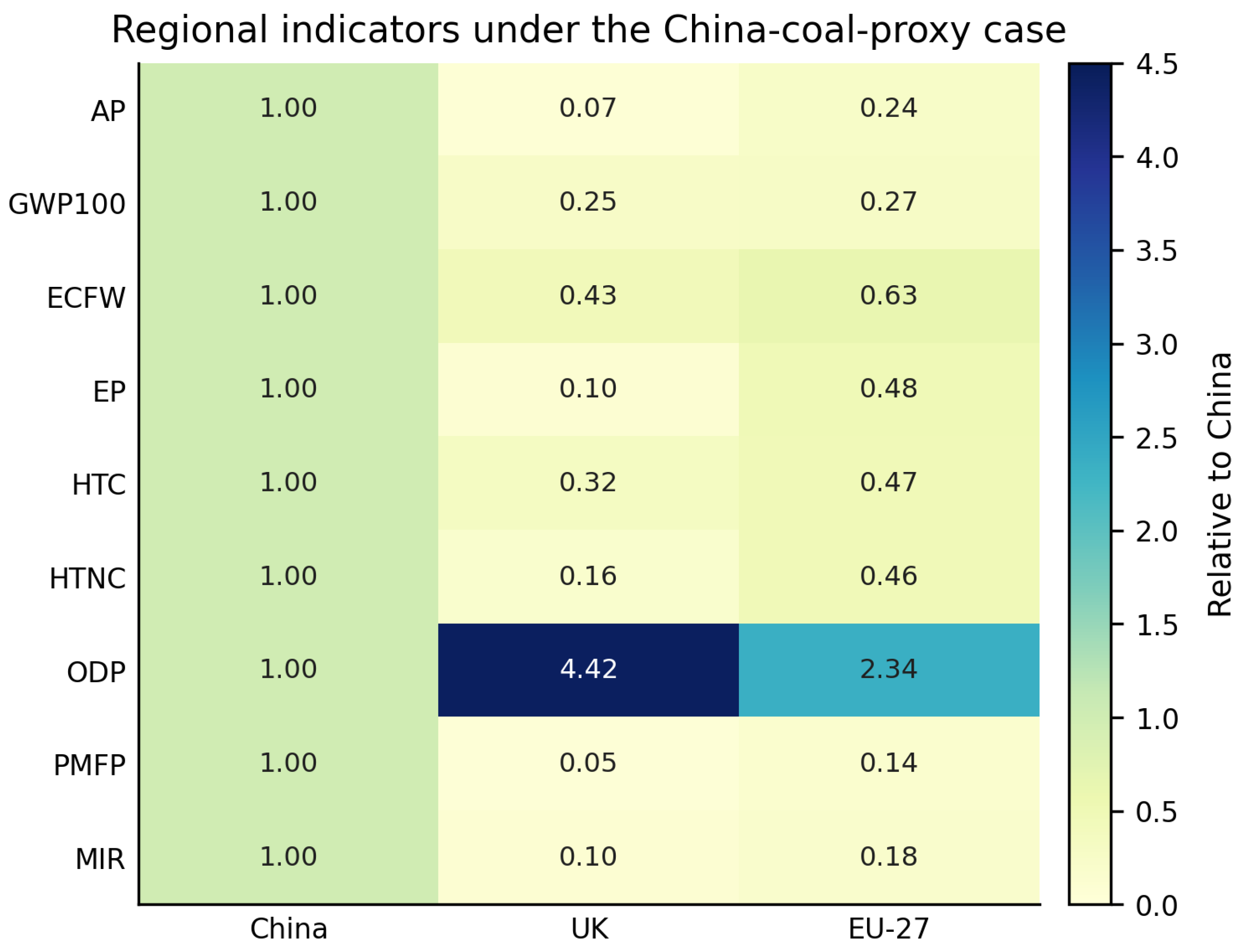
Regional multi-indicator results likewise show that climate-change performance cannot stand in for the remaining environmental categories. Figure 7 shows the regional indicator results under the China-coal-proxy case, with all values normalized to China = 1. When China is normalized to 1, the UK and EU are lower than China for GWP100, AP, EP, PMFP, photochemical ozone formation, freshwater ecotoxicity, and both human-toxicity indicators. ODP is different: the UK and EU relative values are 4.42 and 2.34. The core-six contribution decomposition indicates that gas contributes 95.26% of UK ODP and 83.18% of EU ODP. This striking result is produced by the combination of the UK gas share and the selected gas-process ODP factors under the common UK background; it may reflect genuine upstream supply-chain burdens, technology mapping, or both. Because gas is represented by a UK ecoinvent proxy rather than a region-specific gas inventory, the result should be read as a mapping-sensitive diagnostic, not as evidence that UK or EU gas supply chains universally have these ODP values. Reducing coal generation can strongly improve GWP100 and several conventional pollution-related indicators, but carbon improvement does not guarantee that all non-carbon indicators move in the same direction.

The core-six version excludes oil, bioenergy, and other renewables. Residual-category completion tests whether that omission changes the main inference. Other renewables use low, central, and high indicator-wise values from the existing renewable proxy pool. Oil uses a natural-gas factor, a gas–coal combination, and a UK coal factor as low, central, and high cases. Bioenergy uses a renewable proxy pool, a renewable–gas combination, and a gas–coal combination. These are category-omission sensitivity tests; the proxy coefficients are not region-specific life-cycle inventories.

Table 15. GWP100 after residual-category proxy completion under the China-coal-proxy case.

Proxy Case	China	UK	EU27	UK/China	EU27/China
Low	0.7420	0.1747	0.2008	23.55%	27.06%
Central	0.7497	0.2197	0.2248	29.31%	29.99%
High	0.7636	0.3091	0.2654	40.48%	34.76%

gives the GWP100 values after residual-category completion.

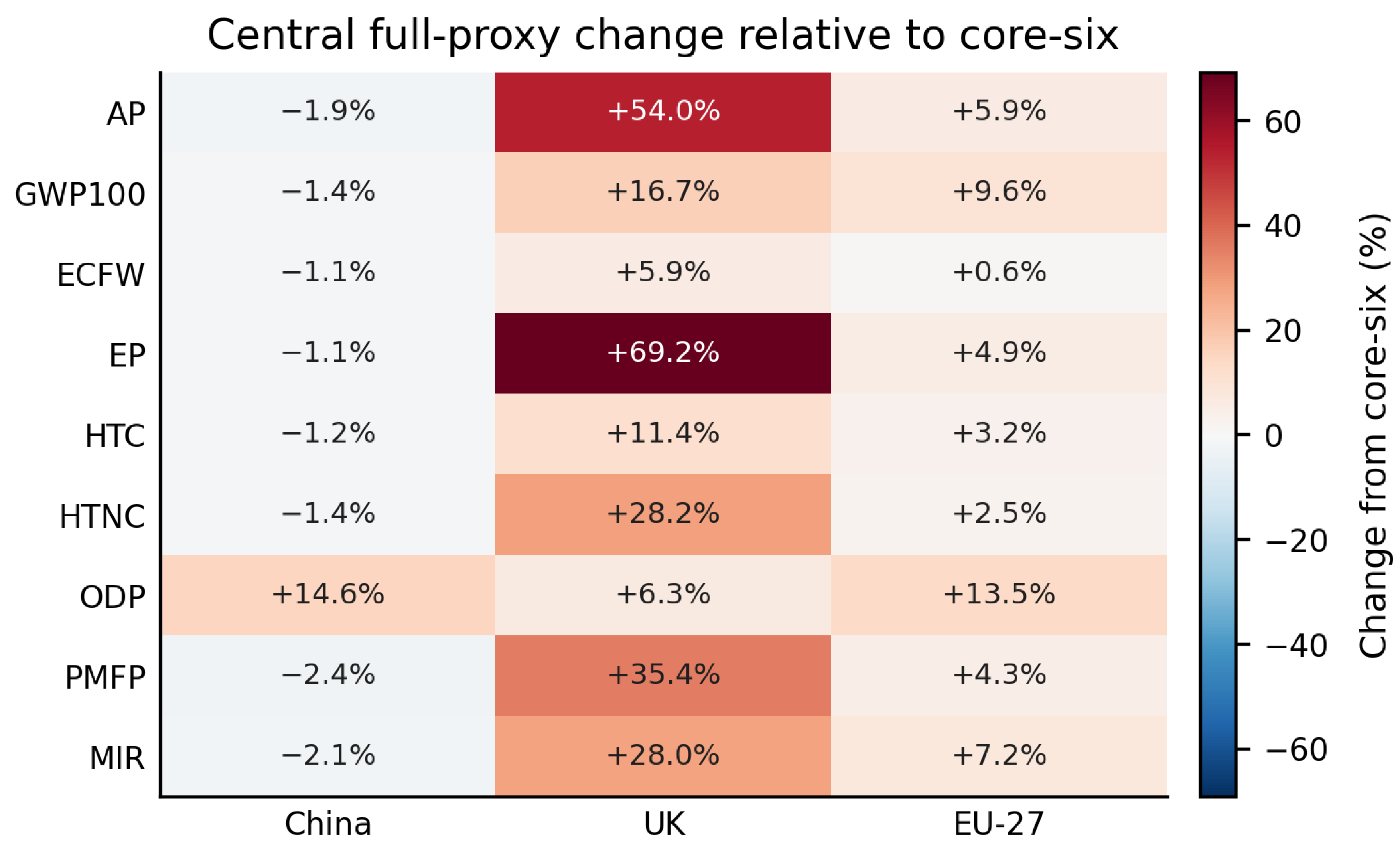
Relative to the core−six results, adding residual categories changes China’s GWP100 by −2.41%, −1.40%, and 0.44% in the low, central, and high proxy cases. Figure 8 decomposes the central-case change by indicator. The corresponding changes are −7.21%, 16.66%, and 64.16% for the UK and −2.10%, 9.62%, and 29.43% for the EU. The difference is mainly driven by the residual−category share: only 2.95% for China, compared with 18.14% for the UK and 9.11% for the EU. China’s absolute result is therefore insensitive to the residual−category treatment, while the UK and EU absolute values carry larger proxy uncertainty.

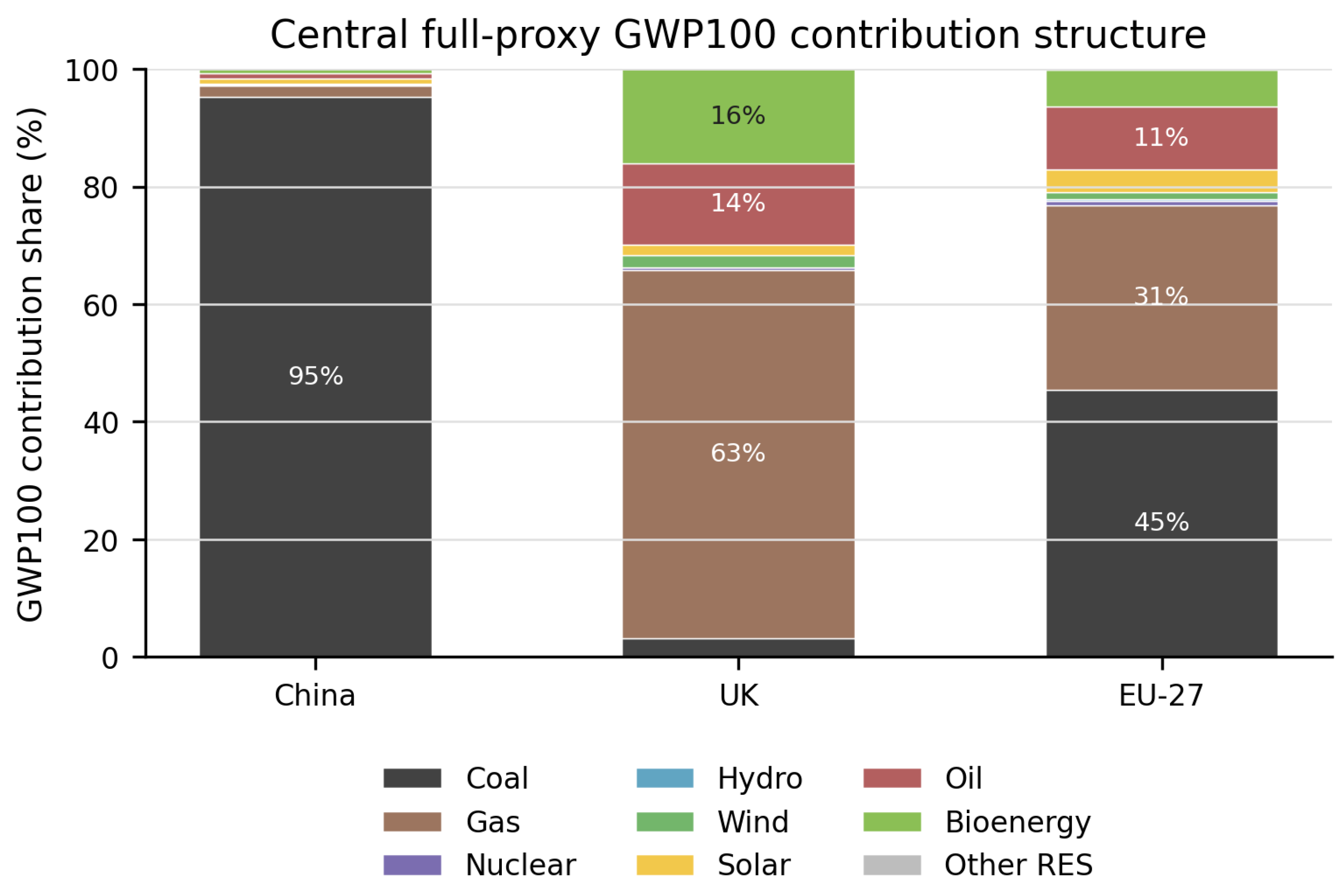
The residual-proxy test leaves the main ranking inference unchanged. Across the three residual-proxy cases, China’s GWP100 ranges from 0.7420 to 0.7636 kg CO₂-eq kWh⁻¹, while the UK ranges from 0.1747 to 0.3091 and the EU from 0.2008 to 0.2654 kg CO₂-eq kWh⁻¹. Even comparing China’s lowest value with the UK and EU highest values, China’s result is still 2.40 and 2.80 times higher. Under the central proxy, coal contributes 95.31% of China’s full-category GWP100, while residual categories contribute only 1.57%. In the UK, gas and residual categories contribute 62.59% and 29.83%. In the EU, coal, gas, and residual categories contribute 45.47%, 31.38%, and 17.08% (Figure 9). Residual completion changes the absolute UK and EU values and their contribution structures, but it does not change the inference that China’s modeled GWP100 is primarily driven by coal generation.

4. Discussion

4.1. Model Robustness and Sensitive Degrees of Freedom

The model separates stable outputs from sensitive degrees of freedom. The most stable output is the climate-change advantage of the low-fossil S2 pathway. Across deterministic calculation, capacity-factor perturbation, PV-boundary perturbation, Monte Carlo simulation, and ReCiPe method comparison, S2 remains the lowest-GWP100 scenario. This performance is not caused by a single low-impact renewable technology; it arises mainly from the reduced generation share of high-impact fossil electricity within the scenario set. The direction of the S2 result is expected because S2 is constructed as the low-fossil stress test; the diagnostic question is therefore the size and sensitivity of the GWP100 margin, not whether a low-fossil stress case ranks lower under a fossil-sensitive indicator. To quantify that margin, the 20,000-run Monte Carlo check gives S2 a mean GWP100 advantage of 0.02143 kg CO₂-eq kWh⁻¹ over S5 (95% simulation interval 0.01961–0.02329); S2 is lower in all sampled draws. Under the literature-factor substitution, S2 likewise remains the lowest-GWP100 scenario in all five literature factor sets, in all 20,000 uniform-range draws, and at all 256 endpoint vertices, with a minimum margin of 0.0137 kg CO₂-eq kWh⁻¹ over the closest competitor (Supplementary Table S11d).

The composite ranking requires a narrower interpretation. Equal weighting, entropy weighting, one-at-a-time sensitivity, PV-boundary perturbation, Monte Carlo analysis, and ReCiPe comparison all show that S2 and S3 are close in composite score. S4 also becomes more competitive when the LCIA method includes additional categories such as ionizing radiation, land use, and water consumption. S2, S3, and S4 therefore constitute a low-burden scenario group rather than a single universal multi-indicator optimum, with S2 the lowest-GWP100 scenario within the tested conditions.

The UK backcast distinguishes arithmetic correction from temporal prediction. Fixed capacity-factor weighting reduces mean generation-share error substantially, and the 2024 fixed-factor GWP100 estimate closely matches the observed-mix calculation. Across earlier years, however, gas utilization changes more rapidly than installed capacity, so a static factor vector can give a larger GWP100 error even while improving overall mix distance. The result strengthens the central generation-weighting argument but narrows its scope: contemporaneous utilization information is needed for annual accounting, while forecasting requires a dispatch-sensitive or dynamically updated capacity-factor module.

4.2. Why Optimization Outputs Are Boundary Diagnostics, Not Planning Prescriptions

The S6–S8 results show the risk of reading linear optimization outputs as direct planning mixes. In the constrained problem tested here, the optimization repeatedly selects PWR, hydropower, and the wind/PV group because those choices are favoured by the current unit impacts and imposed bounds. Hydropower and nuclear upper bounds are active in most or all multi-boundary sensitivity solutions. The active constraints are the central diagnostic finding: environmental optimization is inseparable from the feasible-region definition. A planning interpretation would require additional power-system information, including dispatch, storage, grid, reserve, land, permitting, cost, resource-potential, and reliability constraints.

4.3. Regional Proxy Interpretation and Coal-Displacement Response

The regional proxy exercise provides a structural decomposition of the same weighted-sum logic. The UK and EU do not supply directly transferable generation-mix templates for China; they are reference structures showing different ways to reduce high-impact fossil shares. The UK has nearly eliminated coal generation, but gas still supplies 30.37% of generation and contributes 62.59% of GWP100 under the central full-proxy case. The EU has a lower total fossil share than the UK, but coal remains 9.77% of generation and contributes 45.47% of GWP100 under the same proxy case. Their GWP100 values are therefore similar in the central proxy case, despite different fossil substructures.

For China, the model reports a conditional local sensitivity, not a causal or policy effect: holding total generation and other technology shares constant, transferring one percentage point of generation from coal to technology j changes GWP100 by

$$-\Delta E_{\mathrm{coal}\to j}=0.01(u_{\mathrm{coal},\mathrm{GWP}100}-u_{j,\mathrm{GWP}100}).$$

(8)

Using the China coal proxy and the existing technology factors, a one-percentage-point shift from coal to nuclear, hydropower, or wind lowers per-kWh GWP100 by about 0.0122–0.0123 kg CO₂-eq kWh⁻¹. A shift to PV lowers it by about 0.0116 kg CO₂-eq kWh⁻¹, while a shift to natural gas lowers it by about 0.00784 kg CO₂-eq kWh⁻¹, as shown in

Table 16. Local GWP100 response to shifting one percentage point of generation from coal.

Transfer Direction	Replacement-Technology Unit GWP100 kg CO2-eq kWh−1	Reduction in Electricity GWP100 kg CO2-eq kWh−1
Coal → nuclear	0.00699	0.01230
Coal → hydropower	0.00416	0.01233
Coal → wind	0.01523	0.01222
Coal → PV	0.07895	0.01158
Coal → natural gas	0.45277	0.00784

. These values are static local structural responses under fixed factors. They do not include dispatch, storage, reserve, grid, or market constraints, and they should not be read as annual abatement forecasts.

Within the model boundary, the calculation identifies how a hypothetical coal-to-technology reallocation changes the weighted sum under fixed factors; it does not establish the feasibility, timing, or real-world environmental effect of reducing coal operation. Storage, transmission, flexibility, and other system conditions require separate power-system and regional-inventory assessment. The UK and EU ODP results further show why lower modelled GWP100 cannot substitute for multi-indicator assessment.

4.4. Model Limitations and Future Extensions

The model is intentionally static, attributional, and annual-average. It is suitable for structural diagnostics of generation shares and unit-impact factors, but it is not a dispatch model, capacity-expansion model, market model, or full regionalized electricity-inventory model. The UK backcast covers six matched technology groups and uses annual-average capacity; it does not model plant-level outages, curtailment, merit order, or fuel-price response. The regional results are annual-average structural diagnostics rather than complete regionalized LCAs for China, the UK, and the EU. The China coal factor is a proxy based on 31 provincial hard-coal processes and 2022 provincial thermal-generation weights. Oil, bioenergy, and other renewables are represented by internal low, central, and high proxy cases. Wind is not split into onshore and offshore components for China and the EU. Except for the China coal proxy, most technologies retain UK background factors or S0 aggregate factors. The annual-average weights also omit dispatch, storage losses, reserve capacity, grid constraints, imports, and market behaviour.

Future model extensions should first construct region-specific inventories for China’s provincial coal generation and other major electricity sources, then cross-check modelled intensities against open electricity-carbon-intensity datasets. The annual-average framework should then be coupled to dynamic LCA with renewable curtailment, storage, interregional transmission, and flexible resources. Prospective studies should update the background database consistently with future energy-system scenarios rather than applying present-day inventories unchanged to future mixes [22]. These extensions would turn the present structural diagnostic model into a dynamic regional electricity-LCA modelling platform.

5. Conclusions

This study develops and tests a generation-weighted modelling framework for electricity-mix LCA. Using the lcpy Simple LCA example as a pedagogical baseline, it combines S0–S5 normative scenario simulations, sensitivity and uncertainty tests, S6–S8 optimization-boundary diagnostics, and a 2024 China/UK/EU regional proxy decomposition. The results show which model outputs survive parameter and method changes and which depend on weighting, LCIA method, regional proxy, or optimization boundary.

First, the capacity-to-generation module changes the model output substantially. Installed capacity is not a reliable proxy for per-kWh electricity contribution. Converting S0–S5 capacity shares into generation-weighted shares lowers GWP100 by 13.55–22.59% relative to the capacity-based calculation. In S0, the BWR nuclear share rises from 21.63% to 30.25% after capacity-factor correction, while conventional gas falls from 10.82% to 3.14%. Generation weighting is therefore a necessary step in electricity-mix LCA modelling. The UK backcast provides an observational qualification of this result. Fixed capacity-factor weighting reduces 2020–2024 mean generation-share MAE by 60.1% relative to raw capacity shares, and a lagged annual-factor model reduces it by 72.3%. The close 2024 observed-mix agreement does not extend uniformly across earlier years because gas utilization changes over time. Generation weighting is necessary for structural fidelity, but temporal prediction requires dynamically updated utilization or dispatch modelling. The longer 2015–2024 backcast in the Supplementary Information gives the same direction of result while exposing year-to-year error variation more clearly.

Second, S2 has the most stable climate-change advantage in the S0–S5 scenario set. Its GWP100 is 0.09011 kg CO₂-eq kWh⁻¹, 50.01% below S0, and it remains lowest under capacity-factor perturbation, PV-boundary perturbation, Monte Carlo simulation, and ReCiPe method comparison. Multi-indicator rankings are more sensitive. S2, S3, and S4 should be treated as a low-burden scenario group rather than as a single optimum across all weights and LCIA methods.

Third, the S6–S8 optimization cases show that environmental optima depend on constraint definitions. The model response is dominated by PWR, hydropower, and the wind/PV group, and multi-boundary sensitivity shows that hydropower and nuclear bounds are frequently active. Optimization results should therefore be reported with their boundary sources and sensitivity tests, not translated directly into planning prescriptions.

Fourth, replacing scenario weights with 2024 regional generation shares shows that China’s modelled electricity GWP100 is dominated by coal generation. Under common UK background factors, China, the UK, and the EU core-six GWP100 values are 0.6469, 0.1883, and 0.2051 kg CO₂-eq kWh⁻¹. Introducing the China coal regional proxy raises China to 0.7603 kg CO₂-eq kWh⁻¹. In the central residual-proxy case, China’s full-category GWP100 is 0.7497 kg CO₂-eq kWh⁻¹, and coal contributes 95.31%. Residual-category uncertainty does not change the inference that coal generation share is the dominant modelled structural contributor, but the result remains proxy-based and should not be read as a validated regional inventory.

Overall, low-carbon capacity matters environmentally only when it appears as delivered generation and displaces high-impact fossil generation. For China, the key diagnostic question is therefore how much coal-fired generation is replaced by delivered low-carbon electricity. This conclusion remains bounded by this study’s static, annual-average, attributional, proxy-based design; future work should build regionalized and dynamic electricity LCAs that include dispatch, storage, transmission, and evolving background inventories.