Article

Towards Physics-Informed Neural Networks for Magma-Chamber Cooling: A Case Study of the Rio Pisco Pluton


1
School of Computing, Southern Adventist University, 4881 Taylor Cir, Collegedale, TN 37315, USA
2
Geoscience Research Institute, 11060 Campus Street, Loma Linda, CA 92350, USA
*
Author to whom correspondence should be addressed.
Modelling 2026, 7(3), 92; https://doi.org/10.3390/modelling7030092
Submission received: 6 April 2026 / Revised: 6 May 2026 / Accepted: 11 May 2026 / Published: 14 May 2026
(This article belongs to the Section Modelling in Artificial Intelligence)

Abstract

Magmatic–hydrothermal systems transport heat through coupled conduction and buoyancy-driven fluid flow in porous rock, behavior conventionally modeled with grid-based finite-difference simulators such as HYDROTHERM. We demonstrate that a physics-informed neural network (PINN), built on the NVIDIA PhysicsNeMo framework using automatic differentiation and mesh-free collocation, can produce a stable two-dimensional time-dependent solution for a magma-chamber configuration based on the Rio Pisco pluton in the Peruvian Coastal Batholith. Boundary conditions and material parameters are taken from a prior HYDROTHERM study of the same pluton, and 28 temperature samples digitized from that study are used as a supervised constraint. The PINN couples Fourier conduction, advective heat transport, Darcy flow with a temperature-dependent permeability law, and a mass-conservation formulation; the mass-conservation equation is written in two-phase form, but in the regime studied here, the simulation remains below the boiling curve, so the steam-phase saturation stays at zero and the formulation reduces to its single-phase liquid–water limit. The network reproduces the conductive temperature gradient and a directionally consistent buoyancy-driven flow field, with weaker and less organized circulation than the reference simulation, and a cooling time of approximately 1.6 × 10 5 years, comparable to the ∼175,000 years reported for the matching k = 10 16 m 2 HYDROTHERM reference scenario from which the supervised training data was digitized. We discuss the conditions under which the mesh-free, automatically differentiable PINN approach offers a useful alternative to grid-based solvers.

1. Introduction

Magmatic and hydrothermal systems exhibit tightly coupled thermal and fluid flow processes that control intrusive cooling, crustal permeability, and mineral alteration. Modeling these behaviors requires solving nonlinear partial differential equations (PDEs) for heat transport, Darcy flow, multiphase saturation, and mass conservation. Conventional finite volume and finite element solvers handle these equations with robustness, yet their computational cost increases sharply when simulations extend to long timescales or involve strongly nonlinear two-phase regimes [1]. Limited subsurface observations further constrain attempts to validate long-term geothermal evolution. For instance, HYDROTHERM (https://volcanoes.usgs.gov/software/hydrotherm/, accessed on 10 May 2026) [1], a widely used integrated finite-difference geothermal simulator developed by the United States Geological Survey (USGS), aims to remedy these shortcomings in long-duration multiphase simulations by using fine discretization, small timesteps, and significant computational resources.
Physics-informed neural networks (PINNs) provide a mesh-free alternative to groundwater flow simulators, along with many other types of digital-twin simulators [2]. PINNs embed governing equations and boundary conditions directly into an artificial neural network (ANN) loss function. Individual artificial neurons use infinitely differentiable activation functions, allowing for automatic differentiating of the ANN as a function.
Our contribution is a PINN model for a magma and hydrothermal environment applied to the Rio Pisco pluton in the Peruvian Coastal Batholith. The Rio Pisco pluton is a mid–late Cretaceous intrusion located near Ica within the Arequipa segment of the Peruvian Coastal Batholith, formed during subduction of the Farallon Plate beneath the South American margin. It consists primarily of granitic to dioritic intrusive bodies, and prior field, petrologic, and stable isotope studies have characterized its alteration zones and inferred long-lived magmatic heat input and fluid circulation. González Olivares [3] provides the geometric, thermal, and material parameters used as inputs to our model, as well as the reference HYDROTHERM solution against which we qualitatively compare. The pluton therefore serves as a well-characterized test case for evaluating PINN-based geothermal modeling.
The novelty of this work lies in proposing a mesh-free physics-informed learning approach that can reproduce the long-timescale cooling behavior of a realistic magma-chamber configuration. This work combines a field-constrained geological setting, a simulation window, and tightly coupled conductive, advective, and Darcy-flow physics within a single PINN framework.
This paper is structured as follows. Section 2 reviews prior work on numerical geothermal modeling and PINNs. Section 3 presents the geological configuration, governing equations, and PINN formulation used in this study. Section 4 describes the data sources, ANN architecture, training strategy, and validation procedure. Section 5 reports the PINN’s results. Section 6 presents the discussion. Section 7 presents conclusions and future work.

2. State of the Art

Scientists often rely on grid-based computational techniques—like finite-difference, finite-volume, or finite-element approaches—to explore geothermal and volcanic environments. Simulating how water and steam flow through porous rock and drive thermal transport by both conduction and convection has long depended on these tools, alongside studies of deep magma body solidification [4,5]. One example comes from [6], whose work applied volume-integrated schemes to examine dynamics within silica-rich magma conduits. Ingebritsen et al. [5] tackled large-scale underground water movement driven by thermal gradients, employing porous media flow equations for multiple fluid phases. Cooling patterns of rising magma masses, along with visible geological outcomes across vast plutonic regions, drew the attention of [7].
Recent numerical investigations further illustrate the computational intensity of grid-based approaches for magma-chamber convection. Zambra et al. [8] studied the transient cooling of partially molten basalt within enclosed magma chambers by solving the coupled conservation equations for mass, momentum, energy, and SiO2 concentration under the Oberbeck–Boussinesq approximation. Their formulation incorporated a non-Newtonian power-law rheology calibrated to experimental data and was implemented using a finite-volume discretization with SIMPLE pressure–velocity coupling. Simulations performed for geometries representative of the Peruvian Coastal Batholith yielded cooling times on the order of tens of thousands of years, with conduction remaining the dominant mechanism of heat transport due to the high apparent viscosity of the magma. While such models provide physically detailed and geologically grounded solutions, they require mesh refinement, iterative convergence procedures, and careful numerical stabilization, particularly for Rayleigh numbers approaching 10 13 . These characteristics demonstrate both the rigor and the computational burden associated with classical PDE-based solvers in long-timescale magmatic systems.
Recent geothermal-focused simulations have further emphasized the importance of explicitly modeling phase change during magma cooling. Zambra et al. [8] incorporated latent heat of crystallization through a temperature-dependent phase fraction formulation that modifies thermophysical properties within the mushy zone. Their results demonstrate that narrowing the crystallization temperature range significantly increases total cooling time due to enhanced latent heat storage, highlighting the sensitivity of thermal evolution to phase-transition modeling.
In the context of the analysis of the Peruvian Coastal Batholith, in [3], the author built a thermal representation of the Rio Pisco pluton, applying MATLAB alongside USGS HYDROTHERM code. Data from field geology, isotopic analysis, and rock conditions shaped simulations exploring how heat moves through porous rock–fluid systems across a flat plane. Without water-driven heat transfer, a one-dimensional conduction-only calculation indicated about 210,000 years for the magma body to fall from 900 °C to 600 °C. Once two-dimensional convection of meteoric hydrothermal fluids was included, cooling accelerated and the time to crystallization at the bottom center of the pluton became strongly dependent on host-rock permeability: that research work reports approximately 180 kyr for k = 10 22 m 2 , 175 kyr for 10 16 m 2 , 150 kyr for 10 15 m 2 , and  125 kyr for 10 14 m 2 . The  k = 10 16 m 2 scenario, reporting a cooling time of approximately 175,000 years, is the configuration used as the reference for the present study. The monotonic relationship between permeability and cooling rate reflects how strongly the cooling rate depends on how easily liquid passes through the rock and on the volume of the intruded mass. That research work also reports that other model parameters have a much weaker effect on the cooling time than host-rock permeability: varying the depth of the pluton, the background geothermal gradient, and the pluton size each produces only minor changes in the time to crystallization, while changes in the initial chamber temperature have a moderate effect that is still smaller than that of varying permeability.
Difficulties emerge when standard solvers face larger domains or tightly linked multiphase systems. With growing spatial scales or complex interactions between phases, demand on computing resources climbs quickly—often accompanied by shaky convergence behavior [9,10]. Such issues stand out most in simulations stretching across long geologic periods or those needing fine detail near abrupt temperature changes.
Offering a different approach, PINNs—first presented in [11]—bypass traditional grids by building differential equations right into how error is measured during training. Because of this design, solutions naturally follow physical laws, as these laws are integrated into the ANN’s loss function. These models work well where data is sparse; traditional methods may demand too much memory or be too unstable, or complex hidden values must be uncovered from data patterns easily uncovered using specific ANN architectures. For instance, heat and liquid motion inside sponge-like materials were captured effectively using such methods, thanks to efforts led by [12].
Wang et al. [13] modeled steady-state geothermal gradients in one-dimensional layered domains, while Shukla et al. [14] investigated Rayleigh–Benard convection in synthetic square geometries. There are few studies that incorporate two-phase flow, variable saturation, or nonlinear permeability, and even fewer attempt to model the 10 5 to 10 6 year timescales required to capture the full thermal evolution of intrusive complexes. Temporal stiffness and training instability remain persistent challenges when applying PINNs to geological systems with strong thermal and pressure gradients [15].
To date, no known PINN implementation has attempted to replicate the level of detail achieved in the Rio Pisco pluton model. This includes realistic geological geometries, field-informed boundary conditions, and tightly coupled temperature and fluid flow processes.

3. Model Framework and Geological Configuration

This study combines a simplified two-dimensional geometry, governing physics, and an ANN architecture into a unified PINN framework. Specifically, the geothermal system is represented as a two-dimensional vertical cross-section containing a magma chamber embedded within a porous host rock. The model captures conductive and advective heat transfer, buoyancy-driven Darcy flow with a temperature-dependent permeability law, and a two-phase mass-conservation formulation in which water and steam saturations are tracked separately under boundary conditions applied over geological timescales. In the regime studied here, the system effectively behaves as single-phase liquid water, so the multiphase machinery is exercised only in its single-phase limit.

3.1. Geological Setting

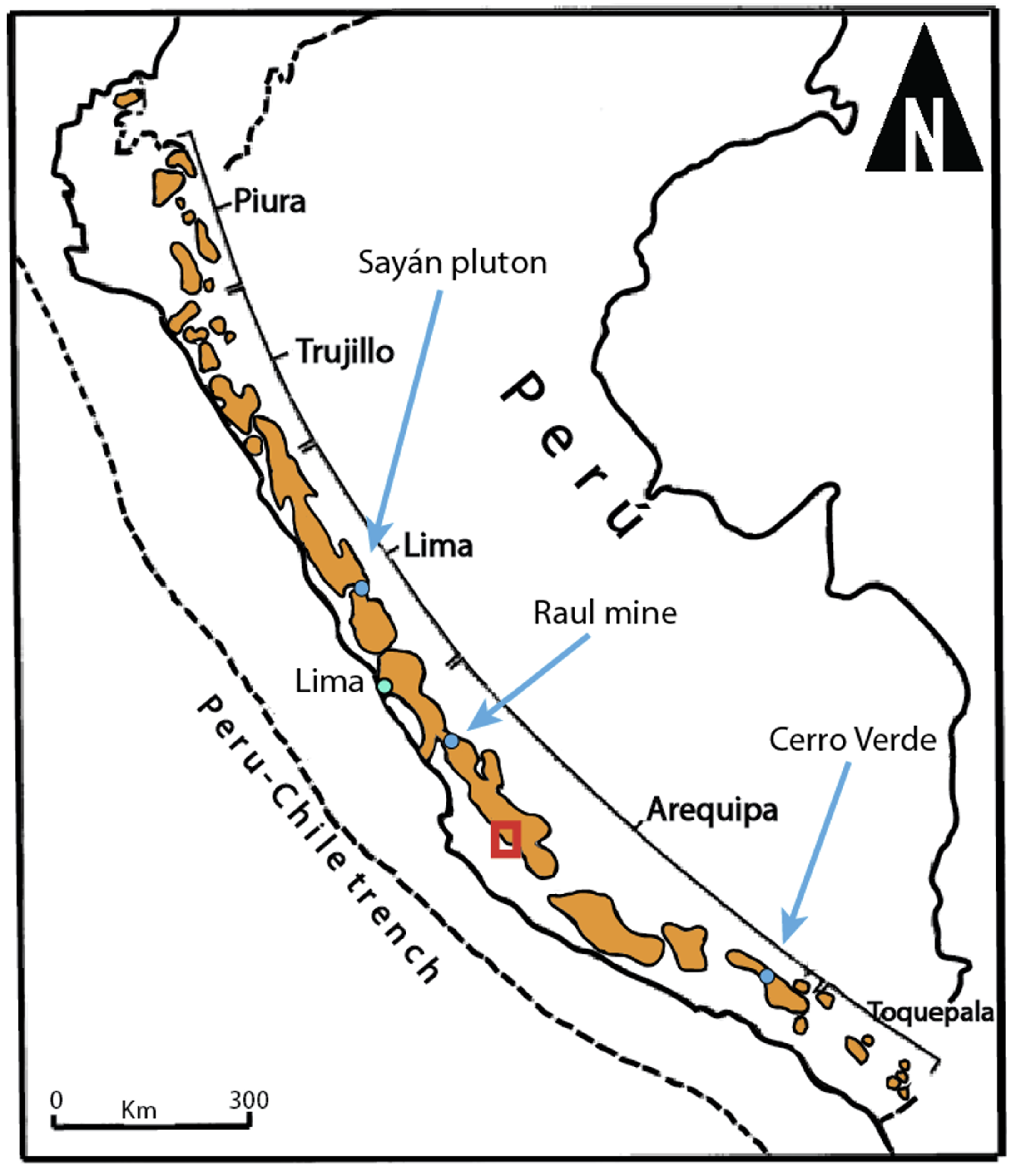
Our PINN model is based on the Rio Pisco pluton within the Peruvian Coastal Batholith. The broad location of this complex is shown in Figure 1, with more details available in [3]. The geological system consists of a shallow crustal intrusion overlain by permeable host rock that supports hydrothermal circulation. The magma-chamber geometry is simplified to a rectangular body embedded within the computational domain. This abstraction preserves the dominant thermal gradients while maintaining tractable model complexity.
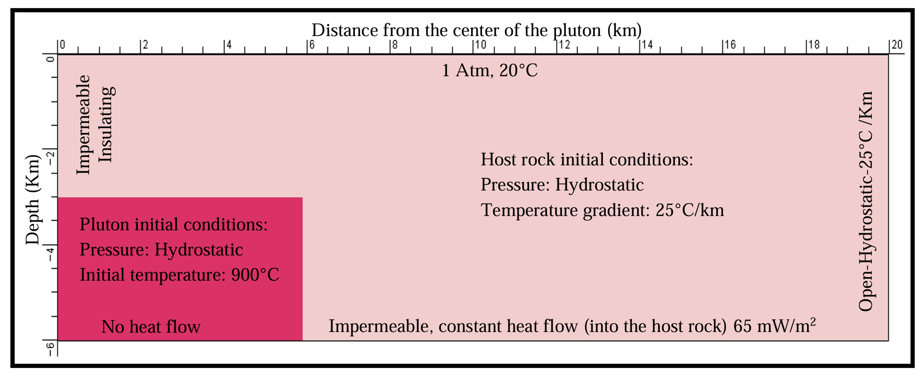
The domain extends vertically from the surface (y = 0) to a depth of 6 km, and horizontally across 20 km, spanning the intrusion and surrounding host rock. The four boundaries are configured as follows. The top boundary fixes the surface temperature at 20 °C and prevents vertical fluid flow. The bottom boundary prevents vertical fluid flow and prescribes a constant upward conductive heat flux of 65 mW/m2, representing background heat input from below. The right boundary imposes a geothermal gradient of 25 °C/km on temperature, ranging from 20 °C at the surface to 170 °C at the 6 km base of the domain, and prevents horizontal flow. The left boundary prevents horizontal flow and is additionally constrained by 28 supervised temperature samples digitized from the HYDROTHERM solution of [3]. The magma chamber’s elevated temperature (900 °C) is imposed as an initial condition over a sub-region in the lower-left of the domain, rather than as a boundary condition.
The magma chamber enters the simulation as an initial thermal anomaly: a region in the lower-left of the domain ( x < 5 km, y > 3.6 km) is initialized at 900 °C, while the surrounding host rock follows a 25 °C/km geothermal gradient. The boundary between the hot intrusion and the surrounding cooler host rock is smoothed by a piecewise-linear ramp, 1000 m wide in the horizontal direction (between x = 5000 and x = 6000 m ) and 600 m wide in the vertical direction (between y = 3000 and y = 3600 m ); the two ramps are combined by taking the maximum of the per-axis interpolation weights, so that points outside the ramp on either axis are fully assigned to the cold side. The chamber is not subsequently held at this temperature—no Dirichlet temperature condition or volumetric source term is applied within the chamber after the initial step—so it cools over the simulated 800,000-year window. The only sustained external heat source is the 65 mW/m2 basal heat flux at the bottom boundary; the top, left, and right boundaries impose sustained Dirichlet temperature conditions that act as a cool sink at the surface and as a fixed background gradient on the side walls. The initial chamber geometry follows the rectangular simplification used in [3] rather than a time-evolving or geologically mapped intrusive geometry. Magma composition, melt fraction, latent heat of crystallization, and crystallization kinetics are not represented in the present formulation; the chamber’s effect on the surrounding rock is captured only through its initial temperature. The model therefore focuses on heat redistribution and buoyancy-driven Darcy flow in the host rock, not on internal magma dynamics.

3.2. PINN

A PINN is an ANN that is bound or informed in some way by physics. This means physical equations are built into the loss function or the structure of the ANN itself [2]. In our case, the PINN approximates the solution fields of temperature, pressure, fluid velocity, and phase saturation as continuous functions of space and time. The network takes spatial coordinates and time as inputs and produces physical state variables as outputs.
Physical laws are enforced by minimizing the residuals of the governing equations evaluated at collocation points throughout the domain. Boundary and initial conditions are incorporated as additional loss terms, ensuring that learned solutions remain physically admissible.
The PINN is implemented using PyTorch version 2.8.0 (https://pytorch.org/, accessed on 13 May 2026) and constructed within the NVIDIA PhysicsNeMo framework version 1.2.0 (https://developer.nvidia.com/physicsnemo, accessed on 10 May 2026). Automatic differentiation is used to compute spatial and temporal derivatives required for evaluating the partial differential equation (PDE) residuals. This means that, after training, any number of samples can be taken from the simulation at a given time, rather than being limited by a grid’s resolution such as in HYDROTHERM. PyTorch supplies automatic differentiation functionality, tensor operations, and GPU acceleration, enabling efficient evaluation of spatial and temporal derivatives required for enforcing the governing equations.
NVIDIA PhysicsNeMo provides a domain-specific abstraction layer tailored for physics-informed learning. It facilitates the definition of PDEs, boundary conditions, and residual loss terms within a unified training pipeline. Governing equations are expressed symbolically and evaluated through automatic differentiation, allowing the model to enforce physical constraints at collocation points distributed throughout the spatiotemporal domain.
The framework also supports modular network architectures and configurable training strategies, which simplifies experimentation with network depth, activation functions, and loss weighting. PhysicsNeMo manages the interaction between physical constraints and ANN optimization, ensuring that conservation laws and boundary conditions are treated consistently during training.
Thanks to NVIDIA PhysicsNeMo, GPU acceleration is employed throughout the training process to handle the large number of collocation points required for resolving long-term geothermal evolution. This implementation allows the network to scale to geological timescales while maintaining feasible training times.
By combining PyTorch and NVIDIA PhysicsNeMo, the model benefits from both low-level numerical flexibility and a high-level physics-aware structure. This integration enables the construction of a physically constrained ANN that remains adaptable to complex geothermal systems.

3.3. Physics Equations

The system is governed by a set of PDEs describing conservation of mass, momentum, and energy in a porous medium. These equations include Darcy flow for fluid motion, Fourier conduction for heat transfer, and advective energy transport by moving fluids. Multiphase behavior is represented in these equations through phase-dependent densities, viscosities, and relative permeabilities. Water and steam phases coexist depending on local pressure and temperature conditions, allowing buoyancy-driven convection to emerge naturally from the governing equations. It should be noted that while the network is formulated to handle multiphase physics, the specific environmental conditions modeled in this study do not cross the boiling curve, meaning the system effectively behaves as single-phase liquid water throughout our simulations.
Heat transfer in geothermal systems occurs through a combination of thermal conduction within solid rock and advective transport driven by fluid motion [5,16]. Conduction dominates in low-permeability regions or at early times before significant fluid circulation develops. This process is governed by Fourier’s law,
q c o n d = K T ,
where q c o n d is the conductive heat flux, K is the effective thermal conductivity of the rock–fluid system, and T is temperature [4,16]. This conductive heat flux term from Fourier’s law is directly incorporated into the energy equation, where it combines with advective heat transport to govern the complete thermal evolution of the system.
As temperature gradients increase and permeability allows fluid movement, buoyancy forces drive convective heat transport. Hot, low-density fluids rise while cooler, denser fluids descend, producing circulation cells that significantly enhance heat transfer efficiency relative to conduction alone [5,17]. In magmatic and hydrothermal environments, this transition from conduction-dominated to convection-dominated heat transport strongly controls cooling rates, alteration zones, and long-term thermal structure [3,7]. Accurately capturing the balance between conductive and convective processes is essential for modeling geothermal evolution on geological timescales [9].

3.3.1. Darcy Flow and Mass Conservation

Throughout this work, the vertical coordinate y is oriented so that + y points downward into the Earth, with  y = 0 at the surface and y = L y at the base of the domain. The unit vector y ^ in Equation (2) therefore points in the direction of increasing depth. Under this convention, gravity acts in the + y direction in physical space, but enters the implementation as the + y -component g = 9.81 m / s 2 of the gravitational acceleration vector relative to the network’s normalized coordinate system; the resulting buoyancy term in the Darcy equation produces upward (i.e., y ) flow of hot, low-density fluid, as expected for hydrothermal convection.
Fluid motion within the geothermal reservoir is described using Darcy’s law, which relates volumetric flux to pressure gradients and gravitational forcing in a porous medium [4,18]:
q = k k r μ ( P + ρ g y ^ ) ,
where q is the Darcy flux, k is intrinsic permeability, k r is relative permeability, μ is dynamic viscosity, P is absolute fluid pressure, ρ is fluid density, g is gravitational acceleration, and  y ^ is the vertical unit vector. Buoyancy forces arising from thermal expansion play a dominant role in driving hydrothermal circulation, generating upward flow above heat sources such as magma chambers and downward recharge in cooler regions [3,9].
The intrinsic permeability k is treated as temperature-dependent to represent the brittle–ductile transition of crustal rocks: cool host rock is permeable enough to support hydrothermal circulation, while hot rock near the magma chamber is effectively sealed. We interpolate k smoothly in log 10 space between a low-temperature value k cold and a high-temperature value k hot via
k ( T ) = 10 log 10 k hot + 1 2 ( log 10 k cold log 10 k hot ) 1 + tanh ( T 0 T ) / Δ T ,
where T 0 is the brittle–ductile midpoint and Δ T controls the sharpness of the transition. Numerical values of all material and scaling constants used in the model are documented in the public source repository (https://github.com/Reno50/SeniorProject-MagmaChamberModeling, accessed on 10 May 2026).
Equation (2) is applied separately to the water and steam phases using their respective phase-specific relative permeabilities, viscosities, and densities, yielding per-phase Darcy fluxes q w and q s [4,10]. These per-phase fluxes enter directly into the mass-conservation equation, which ensures that fluid mass is neither created nor destroyed within the porous medium [4]:
t ϕ ( ρ w S w + ρ s S s ) + · ( ρ w q w + ρ s q s ) = 0 ,
where ϕ is porosity, ρ w and ρ s are the water- and steam-phase densities, and  S w and S s are the corresponding phase saturations [10]. Phase saturations satisfy the closure condition S w + S s = 1 . Changes in pressure and temperature influence phase densities and saturations, allowing boiling or condensation to occur depending on local thermodynamic conditions [17]. This coupling introduces additional stiffness into the system and significantly affects fluid velocities and heat transport [9].
Mass conservation plays a critical role in regulating pressure evolution and ensuring physically consistent fluid redistribution throughout the domain [4,10].

3.3.2. Energy Conservation

Energy conservation governs the evolution of temperature within both the solid matrix and the pore fluids [5,16]. The total energy balance can be written as
E t + · ( q c o n d + q a d v ) = 0 ,
where E represents the combined thermal energy stored in the rock and fluids, q c o n d = K T is the conductive heat flux from Fourier’s law, and  q a d v is the advective heat flux carried by moving fluids [4,10]. Thus, Fourier’s law provides the conductive component of heat transfer that, together with fluid-driven advection, determines the complete thermal behavior of the geothermal system.
Advective transport depends directly on Darcy velocities and phase enthalpies, allowing fluid circulation to redistribute heat efficiently [9]. In multiphase systems, latent heat associated with phase change further influences the energy balance, although explicit phase transition kinetics are not resolved in this formulation [17].
The strong coupling between energy conservation, Darcy flow, and mass conservation gives rise to nonlinear feedback mechanisms that control geothermal convection and long-term thermal evolution [3,7].

4. Materials and Methods

4.1. Materials

We translated values from the results from the HYDROTHERM simulation presented in [3], specifically the modeled heat over time, into data to perform supervised learning with. This data was then integrated into a constraint that was used along with the unsupervised physics-informed learning constraint, among the other constraints. This data is stored with a position value, a time value, and a temperature value, with 28 total samples from the results in [3], shown in Table 1.

4.2. Methods

The architecture of the model shown in this work is almost entirely dictated by the NVIDIA PhysicsNeMo framework. The main component is the solver, which contains the definition of the ANN along with every constraint. These constraints dictate how the network learns physically accurate behavior, initial conditions, and boundary conditions, along with how it learns from training data. The results of each training step are sent from the solver to any validator that is attached to the solver. In our case, we have a single validator, which plots temperature and flow velocity using PyPlot version 3.10.3. The steps used to create the model are as follows, with the source code available online (https://github.com/Reno50/SeniorProject-MagmaChamberModeling, accessed on 10 May 2026).

4.2.1. Formulating the Initial Geometry and Parameterization

The first part of creating a model using NVIDIA’s PhysicsNeMo framework is to create initial geometry and constraints. NVIDIA PhysicsNeMo provides a variety of premade geometries to use as well as the ability to create custom parameterized geometries [2], but our model utilizes a basic rectangle similar to [3]. This geometry definition is shown in Listing 1. Included in this geometry definition is a time parameter on line 5 which allows the network to create a solution for every value of time that we want to sample independently, saving computing costs.
Listing 1. Source code for the chamber geometry.
1 chamber = Rectangle (
2    point_1=(0, 0),
3    point_2=(1, 1),
4    parameterization=Parameterization ({
5        Parameter ("time") : (beginTime, endTime)
6    })
7 )
An important aspect to note about certain large variables is scaling. Numerically small parameters are very important in achieving accurate results using this framework. This is due to the PINN architecture learning much better with smaller (and more uniformly small) numbers. Therefore, in our PINN model, many variables are scaled for network input and then unscaled when working with network output. These variables include all spatial coordinates, which are normalized, temperature, which is scaled down by a constant ratio of 1000 degrees Celsius to 1.0 in the network, and time, which is scaled by a constant ratio of 1 million years to 1.0 in the network.

4.2.2. Building the Deep Neural Network Topology

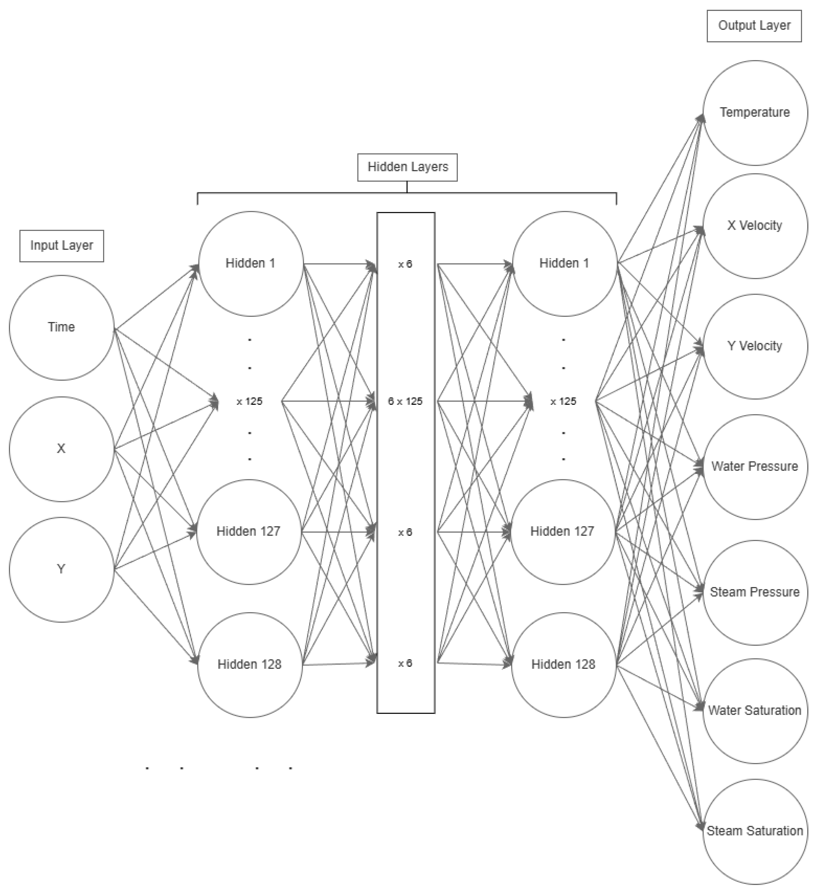
The ANN is defined with the code present in Listing 2 and a visual reference in Figure 2. NVIDIA PhysicsNeMo treats everything to be executed in the forward pass of training as a node. Each of these nodes is a torch.nn.Module wrapper with some additional information, allowing networks to be extended very easily [2]. Each of the keys given in input_keys and output_keys can be included as a dependency to be computed by any node, which is exactly how physics constraints are integrated. These keys are treated as inputs and outputs of a singular network node, with the node hiding the complexity of the network.
Listing 2. Source code for the definition of the ANN.
1 network = instantiate_arch (
2    input_keys=[Key("time"), Key("x"), Key("y")],
3    output_keys=[Key("Temperature"), Key("XVelocity"), Key("
    YVelocity"),
4      Key("Pressure_water"), Key("Pressure_steam"),
5      Key("Saturation_water"), Key("Saturation_steam")],
6    cfg=cfg.arch.fully_connected
The ANN in the model is composed of a fully connected neural network with 8 intermediate layers of 128 artificial neurons each, meaning each neuron is connected to every neuron in the previous layer and every neuron in the next layer. This fully connected structure is also provided by the NVIDIA PhysicsNeMo framework, along with a variety of other network topologies. None of these other topologies seemed to measurably improve results from our testing, so we used the fully connected topology. Our ANN contains three input variables and seven output variables in total. The input variables are an x coordinate, a y coordinate, and time. The output variables are temperature (T), the horizontal and vertical components of the Darcy velocity ( u x , u y ), water and steam pressures ( p w , p s ), and water and steam saturations ( S w , S s ). The steam-phase pressure and saturation are exposed as explicit outputs to keep the formulation symmetric between phases, but  in the regime studied here, no steam is present: the steam saturation stays at zero throughout the domain, and the steam pressure is a free output of the network with no physical role to play.
The activation function and weight initialization scheme are the PhysicsNeMo fully_connected defaults and are not overridden in our configuration file (SiLU (Swish), hidden layers; linear output; Xavier (Glorot) uniform; biases zero). We use the Adam optimizer with an exponential learning-rate decay (Table 2).

4.2.3. Integrating Physics

To evaluate loss during training, the output nodes of the model’s ANN are integrated into a PDE system. NVIDIA PhysicsNeMo’s node system allows easy integration of these equations as PDE-based constraints, and defining equations such as the mass-conservation equation is done programmatically. In Listing 3, we set up the input keys of the network as variables to work with. Line 1 contains the independent variables, which are the network’s inputs. Line 2 contains an example of a primary field function that is dependent on the independent variables, which are network outputs.
Listing 3. Source code for the input and output keys.
1 time, x, y = Symbol("time"), Symbol("x"), Symbol("y")
2 T = Function("Temperature")(time, x, y)
3 # etc....
To use these variables to create output equations, these input keys can be treated as normal variables, and normal operations can be performed to create equations. For example, Listing 4 shows how the mass equation is defined. In line 1, we use a variable to store the mass storage term of the equation, and then in line 2, we use this in the full mass equation and assign it as an output on line 3.
Listing 4. Source code for output equations.
1 mass_storage = phi ∗ (rho_w ∗ S_w + rho_s ∗ S_s)
2 mass_eq = mass_storage.diff(time) ∗ dt_factor + (div_rhoq_w +
    div_rhoq_s) − q_sf
3 self.equations["mass_conservation"] = mass_eq
The two physical balance laws driving the model are mass conservation and energy conservation. The energy conservation equation encapsulates the thermal-transfer component of the expected behavior, combining Fourier conduction with advective transport by the moving fluid. The  mass-conservation equation, expressed in terms of the per-phase Darcy fluxes, simulates the groundwater-flow and mass-transfer components. The formulation tracks both a liquid-water phase and a water-vapor (steam) phase so that boiling and condensation could in principle occur; in the simulations reported here, the conditions remain below the boiling curve, so only the liquid phase is active in practice.
None of the PDE classes shipped with NVIDIA PhysicsNeMo cover this two-phase porous-flow setting directly, so we implement the system as a custom PDE class that inherits from physicsnemo.sym.eq.PDE and registers each residual via self.equations[…], as shown in Listing 4. In addition to the two main balance laws, this class registers auxiliary closure relations: per-component Darcy residuals tying the velocity outputs to the pressure gradient and gravitational forcing, the vertical conductive heat flux used by the bottom-wall basal-flux constraint, and a saturation-sum residual enforcing S w + S s = 1 .
Constraining the residuals for these equations becomes straightforward, as they are defined through a custom PDE interface. Listing 5 presents the specification of residuals of these equations. Lines 2 and 3 specify the nodes and geometry for the constraint, and lines 4 through 10 set the residuals of all of the equations to zero. Line 11 sets the number of samples to take of the interior to evaluate the loss of a given training pass. In lines 12–18, a weighting is assigned to each residual. This relates to how much weight each of these residuals has on the loss function of the network.
Listing 5. Source code for the interior constraint.
1interior = PointwiseInteriorConstraint(
2    nodes=nodes,
3    geometry=chamber,
4    outvar={
5    "mass_conservation": 0,
6    "energy_conservation": 0,
7    "darcy_x": 0,
8    "darcy_y": 0,
9    "sat_sum": 0,
10    },
11    batch_size=cfg.batch_size.interior,
12    lambda_weighting={
13    "mass_conservation": 5.0,
14    "energy_conservation": 5.0,
15    "darcy_x": 10.0,
16    "darcy_y": 10.0,
17    "sat_sum": 3.0,
18    }
19)
In addition to the interior constraint, this model has the following other constraints, as shown in Figure 3:
  • A left-wall constraint restricts horizontal flow past the left wall throughout all times.
  • A top-wall constraint restricts vertical flow past the top wall as well as restricts temperature to be 20 degrees Celsius at the top of the chamber.
  • A right-wall flow constraint enforces u x = 0 across the right boundary. A separate right-wall thermal constraint, applied on a fixed deterministic ( x = 1 , y , t ) grid, imposes the geothermal gradient T ( y ^ ) = 20 + 150 y ^ [ C ] , where y ^ [ 0 , 1 ] is the normalized depth coordinate. In physical units, this corresponds to 25 °C/km, ranging from 20 °C at the surface to 170 °C at 6 km depth, matching the boundary condition reported in [3].
  • A bottom-wall constraint restricts vertical flow past the bottom wall as well as specifying a vertical heat flux upwards of 65 mW/m2.
  • A pressure anchor pins both phase pressures to zero, p w = p s = 0 , on a small square [ 0.49 , 0.51 ] 2 at the center of the normalized domain, evaluated only at the initial instant ( t [ 0 , 10 16 ] in normalized time). Because Darcy’s law depends only on pressure gradients, this anchor fixes an otherwise-free additive gauge so that the network can learn a well-posed pressure field; it is not a sustained boundary condition during the simulation.
  • An initial-interior constraint restricted to the time window t [ 0 , 0.001 ] (i.e., 0– 1 kyr in physical units) provides the network with a consistent starting state. It pins the temperature field to generate_initial_temps ( x , y ) —the discretization of the chamber geometry—and additionally fixes p w = p s = 0 , S w = 1 , S s = 0 , u x = 0 , and  u y = 0 .
  • Geological data constraint contains temperature data taken from [3] directly and encourages the model to match these temperatures on the left wall.

4.2.4. Training Strategy

Training proceeds by drawing fresh batches of collocation points from each constraint’s geometry at every optimizer step and minimizing a weighted sum of mean-squared-error residuals. The optimizer, learning rate, and total step count are listed in Table 2; the remaining details—loss function, residual weights, sampling, and  validation infrastructure—are described below. Our config.yaml overrides only the architecture size, optimizer learning rate, scheduler parameters, batch sizes, and total step count. All other implementation choices (SiLU activation, Xavier weight initialization, MSE per-term loss, plain-sum aggregation, pointwise stochastic sampling) inherit from the PhysicsNeMo 25.08 defaults.
  • Loss Function and Residual Weights
The training loss follows the default behavior of the PhysicsNeMo framework [2]. At every optimizer step, each constraint samples a batch of collocation points; for each point, every residual declared by that constraint (the PDE residuals, boundary mismatches, initial-condition mismatches, and supervised-data mismatches) is evaluated and squared. These squared residuals are averaged within each batch, multiplied by a fixed per-residual weight λ , and  then summed across all constraints to produce the total loss that gradient descent minimizes. The weights are assigned manually and remain fixed throughout training; no adaptive weighting scheme such as NTK weighting, GradNorm, or SoftAdapt is used.
The hand-tuned weights are reported in Table 3, Table 4, Table 5 and Table 6, covering boundary, interior PDE-residual, initial-condition, and supervised-data terms, respectively. The weight λ controls each term’s contribution to the total training loss: a residual with λ = 10 is penalized ten times more strongly than one with λ = 1 , compensating for differences in the natural magnitude of each variable.
  • Sampling Method
Training uses pointwise stochastic resampling: at every step, a fresh batch of collocation points is drawn from each constraint’s geometry. There is no fixed dataset and no concept of an epoch—each optimizer step performs one update on independently sampled points. Per-constraint batch sizes and sampling types are listed in Table 7.
The spatial domain [ 0 , 1 ] × [ 0 , 1 ] maps to a physical chamber of L x = 20 , 000 m wide by L y = 6000 m tall. The temporal domain is normalized so that the network input t [ 0 , 0.8 ] corresponds to 0–800,000 years (timeScalingFactor  = 10 6 ). Temperature is normalized by tempScalingFactor  = 10 3 , so a network output of 1.0 corresponds to 1000 °C.
  • Validation and Visualization
PhysicsNeMo’s validator system takes the form of an abstract class that exposes the inputs and outputs of any node in the training graph, allowing user-defined validators to be attached to a running model. We implement a validator that uses Matplotlib’s pyplot to plot the network’s predicted temperature and velocity fields at fixed time slices and a logger that records the per-key loss at every recording interval to aid debugging and hyperparameter tuning. The  visualization validator uses 21 fixed time slices: 17 evenly spaced at Δ t = t end / 24 from t = 0 to t = 16 t end / 24 , followed by 4 slices at { 18 , 20 , 22 , 24 } t end / 24 . Each slice is paired with 2048 interior points sampled uniformly at random from the chamber domain at initialization and held fixed thereafter, so the validator reports the same spatial sample at every recorded time. The  cooling-time monitor likewise uses 100 time slices and 512 spatial points drawn once from the same uniform distribution over the chamber.

4.2.5. Model Assumptions and Limitations

Several simplifying assumptions were adopted to maintain tractability. Material properties such as permeability, porosity, and thermal conductivity are treated as spatially uniform. Chemical reactions, mineral precipitation, and mechanical deformation are not included.

5. Results

The results reported in this study were trained on a single NVIDIA RTX 6000 Ada GPU with 48 GB of onboard memory. The final configuration, consisting of 50,000 optimization steps, required approximately 5 h per run. All training and checkpoint data were stored on local M.2 NVMe solid-state storage to ensure consistent input–output performance during optimization. Additionally, model checkpoints were saved periodically during training to support recovery, inspection of intermediate states, and comparison across experimental runs. The training run uses ∼15 GB of GPU memory (about 30% of what is available), 7 GB of RAM, and 3% of the CPU.

5.1. Network Loss

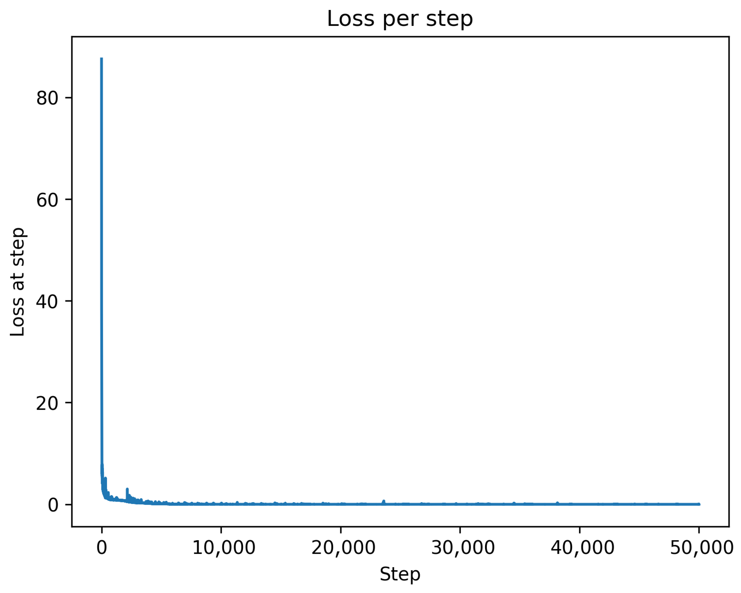
Figure 4 shows the total loss of our model over the 50,000 steps of training performed. All of the constraints included in the previous section, with an emphasis (via a higher lambda weighting) on the physical equation constraints, make up the loss function of the ANN. The steep decline in loss during the early training phase indicates aligning outputs roughly with physical constraints, quickly lowering the loss. After this phase, the model slowly refines its output to match finer details and constraints until it reaches the end of training.

5.2. Predicted Cooling Time Compared to Previous Work

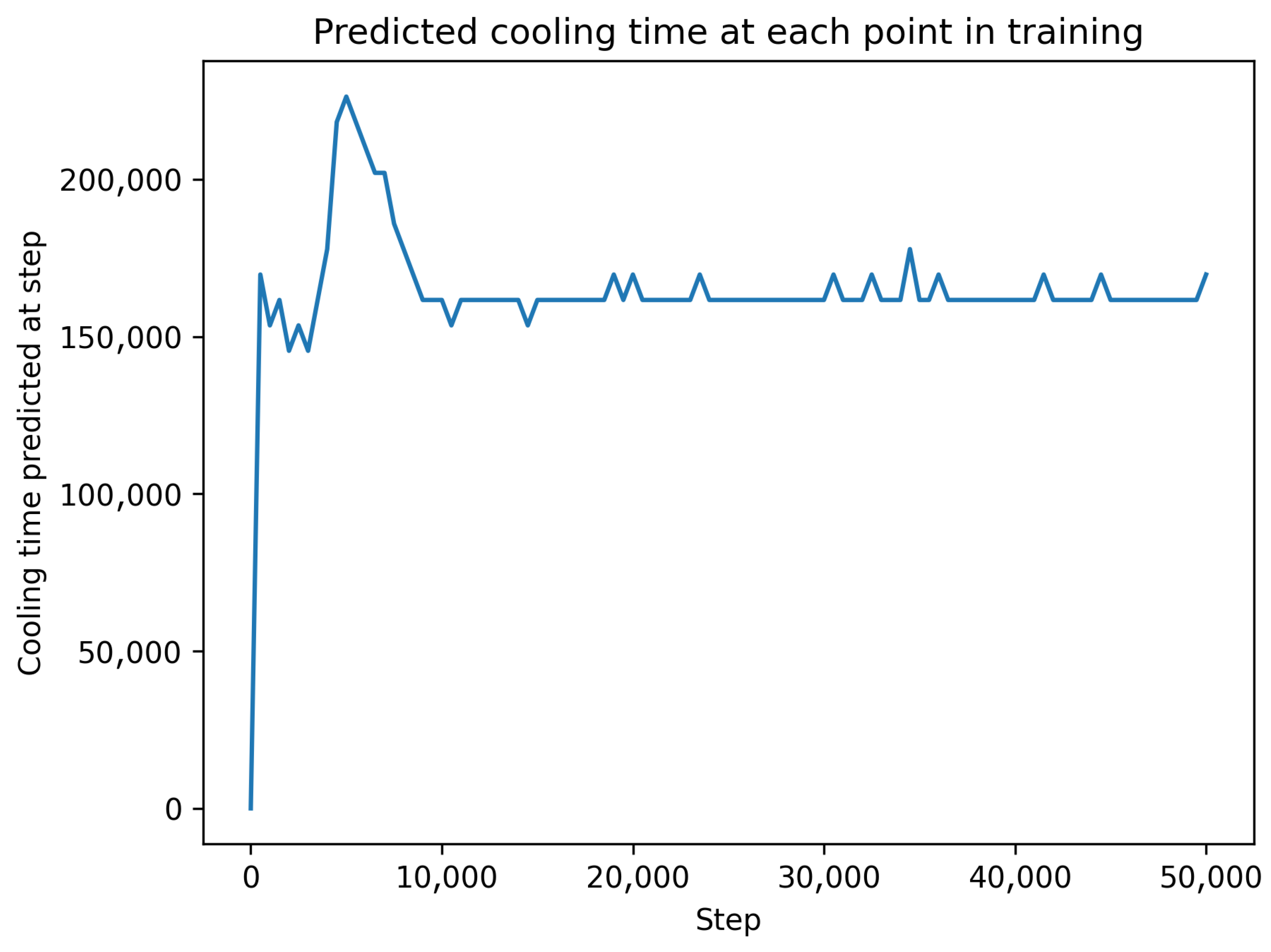
In ref. [3], the temperature of full magma crystallization and increased rock permeability was assumed to be 600 °C. Our model adopts the same crystallization threshold; Figure 5 shows the cooling-time prediction tracked at every step of training. The PINN’s predicted cooling time settles at approximately 162 kyr, which we report below as 1.6 × 10 5 years to reflect the resolution of the cooling-time monitor. The matching HYDROTHERM reference scenario is the k = 10 16 m 2 case from which the supervised training data of Table 1 was digitized; that scenario yields a cooling time of approximately 175 kyr, so the PINN underestimates the reference value by roughly 13 kyr.
A subtlety of the present formulation is worth noting explicitly. The PINN’s PDE residual uses a temperature-dependent permeability law (Equation (3)) that smoothly interpolates between k hot = 10 22 m 2 inside the brittle–ductile zone and k cold = 10 14 m 2 in the cool host rock outside it. Below the brittle–ductile midpoint T0 = 400 °C, where most of the host rock resides for most of the simulation, this law assigns the host rock a permeability two orders of magnitude higher than the constant k = 10 16 m 2 used to generate the supervised data. According to [3], that higher permeability would correspond to a HYDROTHERM cooling time of approximately 125 kyr, whereas the supervised data corresponds to approximately 175 kyr. The PINN’s predicted 162 kyr therefore falls between these two reference values, which is consistent with a residual tension during training between the supervised loss (pulling the solution toward the 175 kyr profile) and the PDE residual evaluated with k cold = 10 14 m 2 (favoring the faster 125 kyr cooling). A more rigorous benchmark would either use k cold = 10 16 m 2 in the PDE to match the supervised data or use supervised data digitized from the k = 10 14 m 2 scenario; we identify achieving this internal consistency as an important refinement for future work.
The cooling-time monitor evaluates the network at 100 linearly spaced time slices across the 800,000-year simulation window, giving an inter-slice spacing of Δ t 8080 years. The reported value is therefore the closest grid point at which the predicted maximum temperature first falls to or below 600 °C, and it should not be interpreted as having six significant figures of accuracy: the underlying resolution is ± 4 kyr. A finer monitor grid (or a continuous root-find on the predicted max x T ( x , t ) field) would tighten this bound but is unlikely to change the order-of-magnitude comparison with [3].

5.3. Predicted Temperatures and Velocities Compared to HYDROTHERM Results

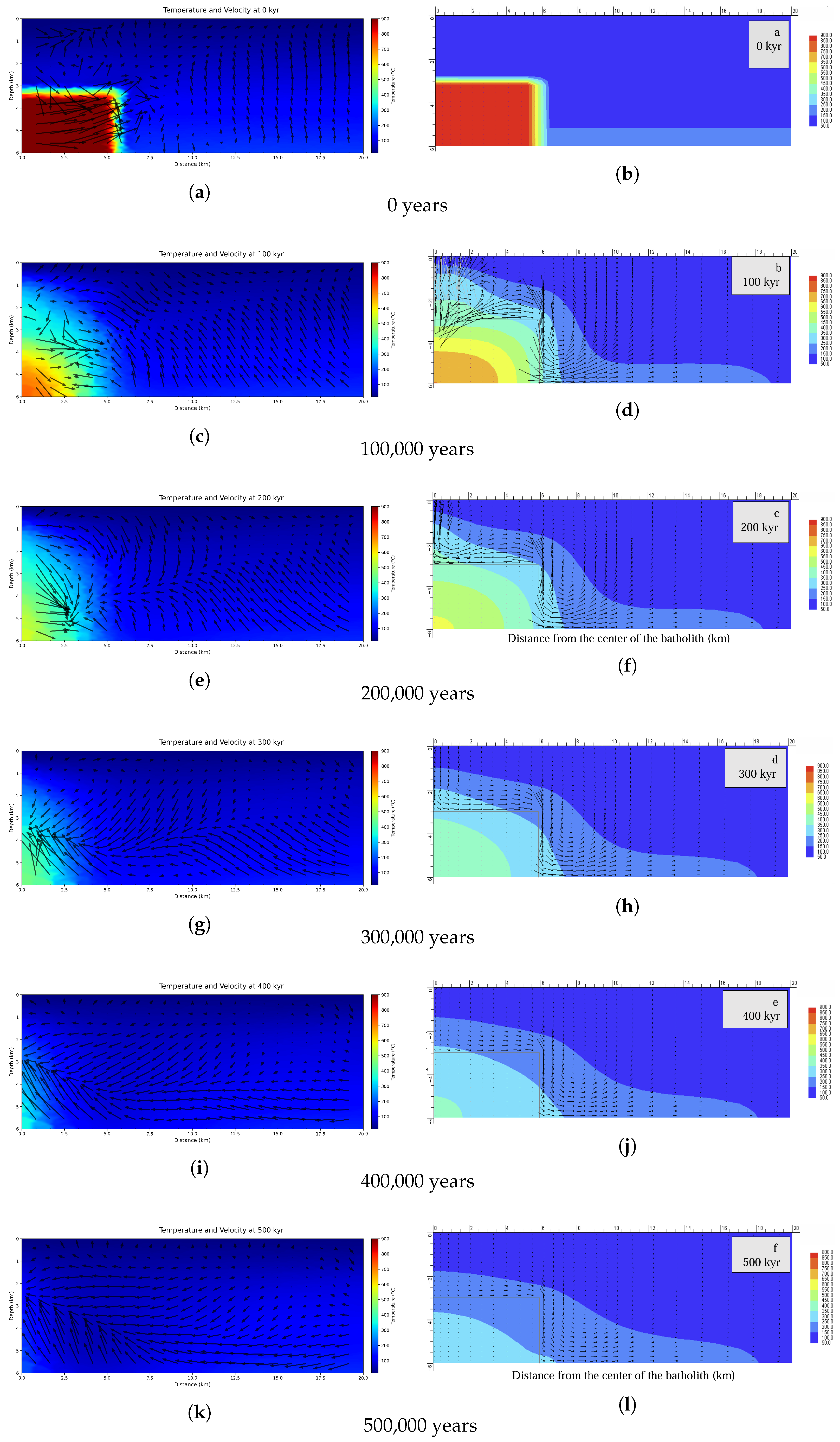
Figure 6 shows a qualitative comparison between our PINN model and the HYDROTHERM model from [3]. The contrasting study does not report the original dataset used in the experiments, explicit runtime, or computational cost figures for the HYDROTHERM simulation. Therefore, a direct numerical comparison of computational efficiency between the two approaches is not possible. On the left column, outputs from the PINN model are shown, and on the right column, outputs from the model in [3] are shown. An important note to consider in this comparison is that our PINN visual output shows arrows to indicate the direction of fluid and gas flow, whereas in [3], where HYDROTHERM was used, lines originate at a point and are directed in the direction of the flow.

6. Discussion

Our PINN model produces approximately qualitative equivalent albeit varying results compared to [3] using HYDROTHERM, as shown in Figure 6. There are clear differences, however, and at nearly every training step beyond the early-spike phase shown in Figure 5, the PINN’s predicted cooling time is approximately 13 kyr shorter than the matching k = 10 16 m 2 HYDROTHERM reference. During training, the model consistently shows a spike at lower steps as it learns more precise details, but evens out to a cooling time of approximately 1.6 × 10 5 years (within the ± 4 kyr resolution of the cooling-time monitor; see Section 5.2).
As for the temperatures and velocities within the chamber over time, our model shows similar results when compared to the HYDROTHERM model used in [3]. At 0 years after the intrusion, shown in Figure 6a, the model accurately captures initial temperature conditions. At 100,000 years in Figure 6c, our model begins to differ from the model in [3], in Figure 6d: rather than holding the hot intrusion’s initial shape, the hot intrusion in our model shrinks much more horizontally. The vertical heat profile remains very similar at this time between the model in [3] and this model. The velocity throughout the cooler parts of the chamber is directed more upward in our PINN approach compared to [3], but it is still directed towards the warm intrusion in both models. At 200,000 years, the vertical temperature profile of the hot intrusion in our model shown in Figure 6e is still very similar to the model found in [3], as shown in Figure 6f, but it has again shrunk horizontally. The velocity continues to differ in similar ways between our model and the model found in [3] as well, with the flow in our model primarily being towards the top of the intrusion. This trend continues for the next three time frames with little difference. At 300,000 years, shown in Figure 6g,h, the hot intrusion has once again shrunk horizontally in our model. Heat is also distinctly concentrated towards the bottom of the chamber, similar to [3]. Once again, the velocity is different between the PINN model and the model in [3], as in the PINN model, the velocity has developed a stream of faster velocity at a depth of about 3 km. At 400,000 years, shown in Figure 6i,j, the hot part of the intrusion has significantly shrunk in both our model and the model found in [3]—the PINN model still shows a thinner heat profile for the intrusion, maintaining a similar vertical heat profile once again. At 500,000 years, shown in Figure 6k,l, both models show the heat of the intrusion as mostly dissipated. Our PINN model shows substantially more heat on the right side of the chamber, with the stream of higher velocity remaining as the main difference in velocity between the PINN model and the HYDROTHERM model found in [3].
The PINN approach offers several practical advantages for approximating coupled magmatic–hydrothermal systems, but it also carries trade-offs that should be acknowledged alongside those benefits. On the positive side, the NVIDIA PhysicsNeMo framework provides a modular interface in which governing equations, boundary conditions, and supervised data can be expressed as separate constraints and recombined as the problem definition evolves. The mesh-free formulation also avoids some of the operating-range restrictions of grid-based simulators: HYDROTHERM, for example, places limits on the temperature and pressure conditions it can resolve [1], and it does not natively accommodate features such as variable magma viscosity, which was consequently omitted in [3]. PINNs do not impose these particular constraints, and once trained, they provide a continuous spatiotemporal solution that can be sampled at arbitrary resolution. In addition, because the PDE residual itself provides a form of supervision, PINNs can be trained with relatively few labeled data points—in this study, 28 supervised samples.
The aforementioned advantages, however, come with non-trivial costs, such as the following, as described by [19]. First, the PDEs embedded in PINNs are necessarily simplified and often neglect multiscale effects, boundary complexities, and nonlinear couplings present in the real system. Second, post hoc explainability tools attribute behavior on the basis of statistical correlation rather than physical causation, and the resulting explanations may violate conservation laws or misidentify the dominant mechanisms. Third, and most critically, these errors do not remain isolated: they propagate multiplicatively through the model, and because the resulting predictions remain visually and physically plausible, they can convey a false sense of confidence that traditional numerical methods—with their quantifiable error bounds—do not.

7. Conclusions and Future Work

This study demonstrated that a PINN can simulate the combined thermal and hydrological behavior of a geothermal system modeled after the Rio Pisco pluton, using a two-phase formulation that operates in its single-phase liquid-water limit under the conditions studied here. Specifically, we created a PINN to estimate temperature, pressure, velocity, and saturation fields over an 800,000-year simulation window by embedding the governing equations directly into the loss function.
The PINN model’s predicted cooling time was approximately 1.6 × 10 5 years, comparable to the ∼175,000 years reported in [3] for the k = 10 16 m 2 HYDROTHERM scenario from which both the supervised training data and the qualitative comparison plots were digitized. The PINN’s temperature evolution shows similar cooling of the intrusion but a slightly larger flow of heat from the bottom of the chamber than in [3]. The ANN successfully generated stable and physically consistent temperature and pressure fields, capturing the expected conductive gradients and long-term cooling trends. It also produced consistent velocity and saturation fields: although the two-phase formulation was not exercised in this regime—conditions remained below the boiling curve, so the steam saturation stayed at zero throughout the domain—the network preserved this single-phase structure stably across the full simulation window. When qualitatively compared to earlier HYDROTHERM results, the model somewhat reproduced the expected convection patterns: upward flow above the intrusion and downward recharge at the margins were present, but the circulation cells were weaker and less organized. This suggests that the PINN captured the general structure of buoyancy-driven flow, although with reduced strength due to simpler material properties and loss-weighting constraints.
Several limitations of the present study should be acknowledged. On the physical-modeling side, material properties such as permeability, porosity, and thermal conductivity are treated as spatially uniform, and chemical reactions, mineral precipitation, and mechanical deformation are not represented. The magma chamber itself is captured only through its initial temperature: magma composition, melt fraction, latent heat of crystallization, and crystallization kinetics are not included in the formulation. Although the network is implemented with a two-phase mass-conservation formulation, the conditions simulated here remain below the boiling curve, so the steam phase is not exercised and the system effectively behaves as single-phase liquid water; the multiphase machinery is therefore validated only in its single-phase limit. On the benchmarking side, the temperature-dependent permeability law used in the PDE residual ( k cold = 10 14 m 2 ) does not exactly match the constant permeability ( k = 10 16 m 2 ) used to generate the supervised data, which contributes to the residual tension during training. The cooling-time monitor used to report the predicted crystallization time has a resolution of approximately ± 4 kyr , set by the 100 linearly spaced time slices across the 800,000-year simulation window. The predicted convection cells are weaker and less organized than those produced by the reference HYDROTHERM simulation, indicating that the PINN captures the directional structure of buoyancy-driven flow but underrepresents its strength. Finally, a direct comparison of computational efficiency between the two approaches is not possible from the available data, since [3] does not report explicit runtime or computational cost figures for the HYDROTHERM simulation.
Future work involves moving beyond the visual comparison of temperature and velocity fields used here by introducing quantitative error metrics—such as root-mean-square temperature differences and flow-field divergence measures—that would allow additional validation against reference simulations. A second direction is broadening the physics represented by the model. The two-phase formulation implemented here was not exercised because the simulated conditions remained below the boiling curve; extending the model into the supercritical and two-phase regime would activate the steam-phase machinery already present in the network and allow the study of boiling, condensation, and phase-change-driven convection in shallower or hotter intrusive settings. A third direction concerns the training methodology itself. The present study uses fixed, hand-tuned residual weights and a single fully connected architecture, with no adaptive loss-weighting strategy. Future work could evaluate adaptive schemes such as NTK weighting, GradNorm, and SoftAdapt to determine whether they reduce the residual tension between the supervised loss and the PDE residual. A fourth direction concerns the internal consistency of the benchmark itself: aligning the permeability used in the PDE residual with the value used to generate the supervised training data—either by setting k cold = 10 16 m 2 in the PDE or by digitizing supervised data from the k = 10 14 m 2 HYDROTHERM scenario—would remove the residual tension between the supervised loss and the PDE residual. Finally, future work could explore three-dimensional modeling—in three dimensions, flow patterns gain complexity, directional differences in rock conductivity become traceable, and irregular magma bodies take shape.

Author Contributions

Conceptualization, G.H.A. and B.L.C.; Formal analysis, G.H.A., B.L.C. and A.E.; Investigation, A.E., D.P. and G.H.A.; Methodology, A.E., D.P. and G.H.A.; Project administration, G.H.A.; Software, A.E. and D.P.; Supervision, G.H.A.; Validation, G.H.A. and B.L.C.; Visualization, A.E.; Writing—original draft, G.H.A., A.E. and D.P.; Writing—review and editing, G.H.A. and B.L.C. All authors have read and agreed to the published version of the manuscript.

Funding

This work was supported by the Geoscience Research Institute, grant 2025_B_C2.

Data Availability Statement

Any source code and data used in this study are openly available at https://github.com/Reno50/SeniorProject-MagmaChamberModeling, accessed on 10 May 2026.

Acknowledgments

We thank the Geoscience Research Institute for their financial support for this project.

Conflicts of Interest

The authors of this paper declare no conflicts of interest.

References

  1. Kipp, K.L.; Hsieh, P.A.; Charlton, S.R. Guide to the Revised Ground-Water Flow and Heat Transport Simulator: Hydrotherm Version 3; Technical Report; United State Geological Survey: Reston, VA, USA, 2008.
  2. Hennigh, O.; Narasimhan, S.; Nabian, M.A.; Subramaniam, A.; Tangsali, K.; Fang, Z.; Rietmann, M.; Byeon, W.; Choudhry, S. NVIDIA SimNet™: An AI-Accelerated Multi-Physics Simulation Framework. In International Conference on Computational Science; Springer International Publishing: Cham, Switzerland, 2021; pp. 447–461. [Google Scholar]
  3. González Olivares, L.U. Conduction Plus Convection Heat Flow Modeling for the Linga Complex, Peru. Ph.D. Thesis, Loma Linda University, Loma Linda, CA, USA, 2017. [Google Scholar]
  4. Bear, J. Dynamics of Fluids in Porous Media; Elsevier: Amsterdam, The Netherlands, 1972. [Google Scholar]
  5. Ingebritsen, S.E.; Sanford, W.E.; Neuzil, C.E. Groundwater in Geologic Processes; Cambridge University Press: Cambridge, UK, 2010. [Google Scholar]
  6. Dufek, J.; Bachmann, O. Quantum magmatism: Magmatic processes at conduit scale. J. Geophys. Res. 2010, 115, B07203. [Google Scholar]
  7. Weinberg, R.F.; Sial, A.N.; Pessoa, R.R. Thermal evolution of batholiths and implications for magma emplacement. Earth-Sci. Rev. 2018, 185, 107–129. [Google Scholar]
  8. Zambra, C.E.; Gonzalez-Olivares, L.; González, J.; Clausen, B.L. Temporal evolution of cooling by natural convection in an enclosed magma chamber. Processes 2022, 10, 108. [Google Scholar] [CrossRef]
  9. Ingebritsen, S.E.; Geiger, S.; Hurwitz, S.; Driesner, T. Numerical simulation of magmatic hydrothermal systems. Rev. Geophys. 2010, 48, RG1002. [Google Scholar] [CrossRef]
  10. Pruess, K.; Oldenburg, C.; Moridis, G. TOUGH2 User’s Guide, Version 2.0; Technical Report LBNL-43134; Lawrence Berkeley National Laboratory: Berkeley, CA, USA, 1999.
  11. Raissi, M.; Perdikaris, P.; Karniadakis, G.E. Physics-informed neural networks: A deep learning framework for solving forward and inverse problems involving nonlinear partial differential equations. J. Comput. Phys. 2019, 378, 686–707. [Google Scholar] [CrossRef]
  12. Cai, S.; Wang, Z.; Wang, S.; Perdikaris, P.; Karniadakis, G.E. Physics-informed neural networks for heat transfer problems. Int. J. Heat. Mass. Transf. 2021, 166, 120789. [Google Scholar] [CrossRef]
  13. Wang, S.; Teng, Y.; Perdikaris, P. Understanding and mitigating gradient pathologies in physics-informed neural networks. SIAM J. Sci. Comput. 2021, 43, A3055–A3081. [Google Scholar] [CrossRef]
  14. Shukla, K.; Jagtap, A.D.; Karniadakis, G.E. Parallel physics-informed neural networks via domain decomposition. J. Comput. Phys. 2022, 447, 110683. [Google Scholar] [CrossRef]
  15. Karniadakis, G.E.; Kevrekidis, I.G.; Lu, L.; Perdikaris, P.; Wang, S.; Yang, L. Physics-informed machine learning. Nat. Rev. Phys. 2021, 3, 422–440. [Google Scholar] [CrossRef]
  16. Fourier, J. The Analytical Theory of Heat; Cambridge University Press: Cambridge, UK, 1822. [Google Scholar]
  17. Driesner, T.; Geiger, S. Numerical Simulation of Multiphase Fluid Flow in Hydrothermal Systems. Rev. Mineral. Geochem. 2007, 65, 187–212. [Google Scholar] [CrossRef]
  18. Darcy, H. Les Fontaines Publiques de la ville de Dijon; Victor Dalmont: Paris, France, 1856. [Google Scholar]
  19. Naser, M.Z. Fundamental flaws of physics-informed neural networks and explainability methods in engineering systems. Comput. Ind. Eng. 2026, 212, 111704. [Google Scholar] [CrossRef]
Figure 1. The five segments of the Peruvian Coastal Batholith with locations of previous stable isotope studies indicated in blue and the study area in red [3].
Modelling 07 00092 g001
Figure 2. Architecture of the ANN. Network inputs are shown on the left. There are 8 fully connected layers of 128 artificial neurons each, with two shown. Network outputs are shown on the right.
Modelling 07 00092 g002
Figure 3. A diagram from [3] describing the chamber geometry and constraints.
Modelling 07 00092 g003
Figure 4. A graph of network loss over all 50,000 training steps.
Modelling 07 00092 g004
Figure 5. The predicted earliest time at which the magma chamber is predicted to have cooled entirely to 600 °C or below, plotted against training steps.
Modelling 07 00092 g005
Figure 6. Comparison of temperature and velocity fields at hundred-thousand-year increments from 0 to 500 kyr. The left column (a,c,e,g,i,k) shows predictions from our PINN approach; the right column (b,d,f,h,j,l) shows results from the HYDROTHERM model of [3].
Modelling 07 00092 g006
Table 1. Sampled position, time, and temperature values used for training, digitized from [3], which reports temperature-depth profiles along the symmetry plane through the center of the pluton at x = 0 for a host-rock permeability of k = 10 16 m 2 .
Depth (km)Time (Years)Temperature (°C)
020,00020
120,00050
220,000190
320,000460
420,000730
520,000880
620,000900
0120,00020
1120,000250
2120,000350
3120,000360
4120,000530
5120,000650
6120,000700
0175,00020
1175,000240
2175,000340
3175,000380
4175,000480
5175,000560
6175,000600
0300,00020
1300,000130
2300,000250
3300,000320
4300,000380
5300,000430
6300,000450
Table 2. Optimizer and scheduler settings.
SettingValue
OptimizerAdam
Initial LR 5 × 10 4
β 1 , β 2 , ε 0.9 , 0.999 , 10 8 (defaults)
LR schedulerTensorFlow-style exponential decay
Decay rate0.995
Decay steps10,000
Total training steps50,000
Table 3. Boundary-constraint weights. Velocity targets enforce no-flow normal to the wall.
ConstraintVariable/Target λ
Left wall u x = 0 1.0
Top wallT = 20 °C1.0
Top wall u y = 0 3.0
Right wall u x = 0 1.0
Right wall (geotherm) T = 20 + 150 y ^ [ C ] , y ^ [ 0 , 1 ] 1.0
Bottom wall u y = 0 3.0
Bottom wall q y = − 0.065 W / m 2 3.0
Pressure anchor p w = 0 1.0
Pressure anchor p s = 0 1.0
Table 4. Interior PDE-residual weights (full domain).
Residual λ
Mass conservation5.0
Energy conservation5.0
Darcy (x-component)10.0
Darcy (y-component)10.0
Saturation sum, S w + S s 1 3.0
Table 5. Initial-condition weights, enforced on t [ 0 , 0.001 ] .
VariableTarget λ
Temperaturegenerate_initial_temps ( x , y ) 30.0
p w 0.01.0
p s 0.01.0
S w 1.010.0
S s 0.010.0
u x 0.03.0
u y 0.03.0
Table 6. Supervised-data constraint weight. The 28 records are taken from the digitized HYDROTHERM left-wall profiles of [3] and are listed in Table 1.
ConstraintVariable/Target λ
Geological data T ( 0 , y i , t i ) = T i HT for i = 1 , , 28 5.0
Table 7. Per-constraint sampling configuration. Batch sizes are redrawn at every training step unless marked deterministic. The  pressure anchor is enforced at a single near-zero-width time slice ( Δ t = 10 16 in normalized units) and is therefore effectively an initial-only constraint.
ConstraintGeometrySamplingBatch Size
Left wall ( x = 0 )Boundary lineStochastic4000
Top wall ( y = 0 )Boundary lineStochastic4000
Right wall ( x = 1 )Boundary lineStochastic4000
Right-wall geothermPre-generated ( 1 , y , t ) gridDeterministic4000
Bottom wall ( y = 1 )Boundary lineStochastic4000
Pressure anchor [ 0.49 , 0.51 ] 2 × [ 0 , 10 16 ] Stochastic100
Interior PDE residuals [ 0 , 1 ] 2 × [ 0 , 0.8 ] Stochastic8000
Initial-condition interior [ 0 , 1 ] 2 × [ 0 , 0.001 ] Stochastic8000
Geological data28 fixed recordsDeterministic28
Disclaimer/Publisher’s Note: The statements, opinions and data contained in all publications are solely those of the individual author(s) and contributor(s) and not of MDPI and/or the editor(s). MDPI and/or the editor(s) disclaim responsibility for any injury to people or property resulting from any ideas, methods, instructions or products referred to in the content.