


Abstract
The integration of automated learning and video analysis enables the development of intelligent systems that can operate effectively in uncertain scenarios. These systems can autonomously identify dominant motion dynamics, depending on the theoretical framework used for representation and the learning process used for pattern identification. Current literature offers a state-based approach to describe the key temporal and spatial relationships required to understand motion dynamics. An important aspect of this approach is determining when the number of positively learned rules from a given information source is sufficient to detect dominant motion in automatic surveillance scenarios. This is crucial, as it affects both the variability of movements that monitored subjects can exhibit within the camera’s field of view and the resources needed for effective implementation. This study addresses these gaps through a grammar-based sufficiency criterion, which posits that learning is complete when production rule growth stabilizes, under the assumption of system stationarity. The stability criterion evaluates whether the most probable rules are learned over time, and whenever a high-growth rule is added, it is used to update the criterion. We outline several benefits of having a formal criterion for determining when a symbolic surveillance system has a robust model that explains the observed motion dynamics. Our hypothesis is that a correct model can consistently account for the majority of motion dynamics over time in an automated learning process. The proposed approach is evaluated by modeling motion dynamics in several scenarios using the SEQUITUR algorithm as input and computing the probability of stability along the learning curve, which indicates when the model reaches a steady state of consistent learning. Experimental validation was conducted in real-world scenarios under varying acquisition conditions. The results show that the proposed method achieves robust modeling performance, with accuracy values ranging from 83.56% to 95.92% in dynamic environments.
1. Introduction
In rapidly growing cities, it becomes mandatory to implement video surveillance systems that operate effectively across a range of environmental conditions, both indoors and outdoors. This generates a massive volume of information, which is impossible to analyze comprehensively. From this perspective, it is necessary to integrate intelligent systems that assist in processing this information, with an emphasis on detecting and analyzing events of interest [1,2]. The detection of these events is particularly relevant in applications aimed at crime prevention, tracking persons of interest [3], detecting atypical behavior [4,5], optimizing resource allocation [6], and analyzing crowd dynamics [7].
To address these challenges, motion modeling has increasingly benefited from data-driven approaches that leverage large-scale datasets and advanced representation learning techniques. In particular, recent deep learning methods have shown a great ability to capture complex motion patterns and improve prediction accuracy in dynamic environments [8,9,10]. Despite these advances, most existing statistical, heuristic, and data-driven approaches focus primarily on improving detection or prediction performance, without explicitly determining when sufficient information has been learned. Consequently, the learning process is often guided by empirical criteria or application-specific conditions, lacking a clear and interpretable measure of information sufficiency. A sufficiency criterion determines when the learning process has reached an adequate level of information, while preventing overfitting that may limit the generalization capability of the resulting model. The criterion proposed in this work addresses this limitation by providing a quantitative measure that helps interpret the condition for determining when sufficient information has been learned.
A literature review exhibits the main variables that affect the effectiveness of existing techniques, classifying them as follows:
- The quality of the data collected, since its accuracy and completeness directly impact the effectiveness of the process [11,12,13].
- The frequency of sampling data, referring to the periodicity with which the data is renewed, which significantly influences the ability to detect activities of interest [14].
- Coverage or scope, which determines the susceptibility of events to be detected as a result of the perspective of the cameras and possible occlusions present in the scene associated with the semantics of the dynamic observed [15,16,17].
- The sensitivity of the system, referring to the detection threshold that allows us to distinguish between an event of interest and a possible false positive [18,19,20].
Intelligent surveillance systems employ adaptive machine learning techniques to identify and extract motion structures, enabling the representation of scene dynamics with the aim to provide a useful explanation of the underlying dynamics. In this context, two key aspects are considered: motion representation and structural modeling.
The first aspect addresses how motion data is encoded to ensure a compact representation consistent with object dynamics [9,10,21,22]. Similarly, deep learning-based methods extract features such as object position, aspect ratio, and height [23,24]. The second aspect focuses on the structures used to group and model motion patterns, which can be approached as follows:
- Geometric and aspect-based representation as object geometry, texture, or color, object border contours [8,25,26], while others impose geometric constraints such as length and area through cost functions; for instance, Chen ref. [27] employs convolutional neural networks (CNNs).
- Hierarchical structures based on the enumeration of reference temporal/spatial features [28,29], which use multiscale inference strategies by combining predictions across multiple-level analysis or pyramidal analysis.
Modeling scene dynamics to detect dominant motion patterns is essential for describing activities over time, particularly in automatic monitoring systems that recognize and differentiate observed behaviors [30,31,32]. To this end, various techniques leverage motion information to infer models of such activities.
The effectiveness of these models depends on the underlying learning processes, as the proper definition of motion patterns directly impacts the performance of monitoring and security systems [2]. Consequently, identifying relevant motion patterns is a fundamental task for detecting or filtering events of interest in surveillance scenarios.
Despite significant progress, several tasks still lack general solutions [33,34]. Current efforts address challenges such as missing information caused by random or deterministic factors, motivating the use of imputation techniques like k-nearest neighbors (KNN) and missForest [35]. Additional challenges arise when algorithms require a minimum amount of data for learning or prior knowledge of the number of rules needed to represent the data. In this context, Callaghan et al. [36] emphasize the need for reliable criteria to assess information sufficiency, identifying it as an open research gap. These approaches can be grouped into five main categories:
- Sampling-based criteria, where the amount of relevant information is estimated through random sampling, and the process stops once a predefined target is reached;
- Heuristic-based techniques, where stopping conditions are triggered by detecting a threshold of irrelevant or redundant information;
- Pragmatic criteria, which define a fixed learning time adjusted to the application, often at the expense of efficiency;
- Automatic criteria, which rely on specific metrics and more complex strategies to determine when to stop the learning process;
- Deep learning-based approaches, which learn motion representations from large-scale datasets, typically focusing on improving accuracy rather than determining when sufficient information has been learned.
These limitations highlight the lack of a formal and interpretable criterion for determining information sufficiency, motivating the development of approaches that explicitly characterize how information is progressively acquired during learning.
In this context, representing motion dynamics through symbolic structures provides a natural framework to analyze the evolution and stabilization of patterns over time. This perspective enables the formulation of learning criteria based on the model’s structural evolution rather than solely on predictive performance.
This work introduces a novel sufficiency criterion for assessing the state of the learning process, specifically identifying when the system has acquired the key rules needed to explain a symbolic source. The proposed approach is grounded in the heuristic principle that, for stationary systems, the dominant dynamics can be represented by a finite number of rules, and that changes in stationarity are reflected in the rapid emergence of additional rules.
The system segments the camera’s field of view into regions with high motion probability and classifies them into discrete, connected states, each assigned a unique symbolic label. Over time, sequences of motion symbols are generated and organized into a grammatical structure that models state transitions through an automated inference criterion, as described in [37,38].
This grammatical framework treats the generated sequences as positive samples of the underlying dynamics captured in the video data. As a result, the system models motion dynamics by uncovering recurrent patterns via grammatical inference, while applying a formal sufficiency criterion to determine when learning has reached a stable regime.
In light of the above, the most relevant contributions of this research are the following:
- The definition of a criterion of information sufficiency that determines when the system has reached grammatical stability.
- Criteria that exploit the properties of periodic systems, which are based on information criteria to learn the most significant production rules.
- Discrete model criteria based on the right grammar to symbolically represent movement trajectories in video sequences.
- A criterion to encode a state-based system, considering the different trajectories through the SEQUITUR approach for inferring the grammar structure in the most compact representation of movement patterns.
2. Proposed Model
This proposal describes a state-based model in which each state represents a spatial area of the camera’s field-of-view projection. A set of adjacent and connected pixels defines each state. The states do not overlap, so the activation of a state (an indication of movement) is modeled as a probability distribution over the variability in pixel intensities that compose it. States with a high probability of variability are considered active and may change over time. Thus, the dynamics of an object moving through the scene are expressed as a sequence of state activations over time.
The structures of observable dynamics are characterized by a stack automaton, which enables the hierarchical modeling of object movements as a proper grammar. The grammar representing the movement is constructed using the SEQUITUR algorithm, which infers a hierarchical structure from a sequence of discrete symbols [37]. This approach enables dynamics to be modeled using hierarchical structures, and verifying that the dynamics are associated with the model involves, through the grammar, determining whether the previously defined structures can explain the sequence of activated states.
A workspace V is considered as a grid space representing the two-dimensional projection of the camera’s field of view with dimensions , which, for a particular position , is indexed by . The number of partitions of the workspace is . From these partitions, the current valid state is a partition such that for every tuple , where , there is at least one connected path between both points, and all different states are always disjoint.
Evidence that an object occludes a state, due to temporal contrast in color change, is represented by Equation (1).
The values of and the estimate of P represent the confidence/certainty of motion detection and the process for estimating probability. The function allows us to determine whether the state e has motion or not at time t. Each state is represented by a symbol from an alphabet by a bijection from . Whenever there is positive evidence of moving in a given state , the associated symbol becomes emitted. This process is represented by the function , which is defined in .
The function assigns a unique symbol to each state that has a significant probability of movement. The emitted symbols are denoted by a set of activated states.
The concatenation of emitted symbols by frame over time constructs a string used as positive evidence to infer grammars , considering each emitted string a positive sample of the grammar. These grammars enable the identification of recurring movement patterns, which are expressed through grammatical rules . By applying the properties of SEQUITUR in the generation of rules, it is possible to construct hierarchical representations of the observed behavior.
This discrete formulation captures the incremental growth of the rule dictionary as new symbolic trajectories are incorporated. When the number of rules generated between two consecutive sequences and satisfies , no new structural patterns are discovered in the symbolic representation of the trajectories. At this point, the rule dictionary becomes stable, and the system can be considered to have captured the dominant motion dynamics of the environment.
2.1. Motion Modeling
In the study of computer vision-based learning methods, various techniques have been proposed for representing motion information, as discussed in [31,39], offering interesting approaches for extracting motion patterns. One of these approaches can be represented by the following expression:
where represents the motion information for the objects in the scene, and denotes the intensity of the pixel at position at time instant t. The difference between the intensity values at two consecutive time instants, t and , allows us to estimate the change in the motion. From this information, it is possible to obtain the trajectories of the moving objects, which are represented as the set . The information on the movement pattern generated by an object, throughout a sequence of images at a given time t, is expressed as , where each element corresponds to a spatial position occupied by the i-th object at time t [40].
2.2. Trajectory Generation Process
In the process of trajectory generation, several techniques have been proposed to enhance motion representation, including trajectory binarization [41,42], N-tuples, and symbol strings [43]. Each approach presents specific advantages depending on the application context. Table 1 summarizes representative motion coding strategies, providing a reference framework for positioning the proposed method.
Table 1.
Comparison of movement coding techniques in similar context applications.
Following this analysis, a representation based on symbol strings is adopted [45], which offers an effective solution to the problem of trajectory expressiveness . The new representation of trajectories begins with the definition of regions belonging to the movement E and is formalized by the function , where each trajectory of an object is represented as a sequence of states .
The finite state set is obtained from scene analysis following the method proposed by Garcia et al. [45]. This approach derives motion information from object trajectories using a decay function [46], , to subsequently obtain the history of the displacement information using the following equation:
The information magnitude in depends on the value of the decay factor , defined as follows:
Here, denotes the video acquisition frequency, and the timescale over which motion information is retained. The cumulative sum (see Equation (6)) is calculated using the trajectory information obtained from the scene to obtain a two-dimensional spatial distribution of motion.
High-probability motion regions E are obtained by segmenting using a Watershed transform based on local maxima [47,48,49]. Figure 1b illustrates the resulting pseudocolor map, where high-motion areas appear in yellow and low-motion regions in blue.
Figure 1.
Process for generating path trajectories: (a) Trajectory motion information . (b) Surface generated with trajectory information . (c) State mask .
With the region E defined, it is now possible to take the information on the state mask , Figure 1c, to obtain the movement representation as trajectories S with the following:
Here, the trajectory formed by the new set of regions E is defined as ; by applying , a new trajectory set S is then formed by the interaction of the objects with the state mask resulting from the movement information contained in .
2.3. Grammar Inference
With the symbolic representation of movement through a string of symbols , it is now possible to obtain right grammars, which allow for the representation of movement patterns. A grammar is defined as a tuple , where is a set of terminal symbols, is the set of non-terminal symbols, R consists of the production rules that define how symbols can be transformed, and is defined as the initial rule [50].
Based on the above, given a path , we obtain the right grammar as a result of applying SEQUITUR to [51], where . The associated alphabet is , and the non-terminal symbols are . From this process, it can be observed that the pair of symbols is repeated at the beginning of the sequence. Consequently, SEQUITUR detects this repetition and generates a replacement with a non-terminal symbol , finally generating the production rule . This sequence is transformed into , and it is then observed that the pair of symbols , c is repeated once more on two occasions. This pattern is also replaced by a new non-terminal symbol , thus generating the following production rule . Following the natural order of the process, the sequence is transformed once again, thus resulting in a compact grammar defined as . This process generates the grammar . This extensive process is illustrated in Table 2.
Table 2.
Process for generating grammars with SEQUITUR.
Finally, when a dictionary is created with the production rules generated for , it is possible to reuse them to represent other trajectories with similar structures.
The hierarchical structure shown in Figure 2 illustrates how the SEQUITUR algorithm infers a context-free grammar from a symbolic sequence . In this representation, each node corresponds to a symbol in the derived grammar, either a non-terminal symbol representing a recurrent subsequence or a terminal symbol belonging to the original alphabet. This hierarchical organization enables SEQUITUR to compactly encode structural regularities and temporal adjacencies compactly, thus producing a grammar that models both local motion transitions and global structural dependencies.
Figure 2.
Working of SEQUITUR algorithm to infer grammar.
The grammar inferred by SEQUITUR can be interpreted as a right grammar when the production rules are expanded from left to right. This directional derivation preserves the causal and temporal flow inherent in the motion data, aligning the symbolic grammar generation with the chronological evolution of trajectories . Consequently, the hierarchical generation process of SEQUITUR not only compresses redundant temporal patterns but also emphasizes the dominant trajectory rules that characterize the underlying scene dynamics. This property makes the approach particularly suitable for the grammatical modeling of spatiotemporal processes, in which the balance between structural compactness and temporal expressiveness is essential.
3. Information Sufficiency Criterion
Given the general process of generating right grammars described in Section 2, in which for each symbolic sequence , a grammar , the relationships between the symbol strings , and their respective grammars are analyzed. The objective is to understand how the algorithm’s behavior in generating production rules affects the total number of rules required to represent a given sequence. In this context, the system receives an input string and produces a unique combination of rules that describe it entirely.
This analysis leads to the main contribution of this work: determining the minimum amount of information sufficient in a sequence of symbols to uniquely define its right grammar .
3.1. Movement Paths and Regions
The previous section defined the process for generating trajectories S. These trajectories are composed of information on the movement patterns of , in which each position satisfies . This implies that the elements describing the trajectory of an object may belong to the same region e. Addressing this idea, the following homologous trajectories are proposed: and , where . This condition establishes that, for the trajectory , and using the Levenshtein distance as the metric, it holds that for . This result reinforces the underlying assumption that both representations encode equivalent motion information, allowing them to be described through a shared set of production rules. Under this interpretation, it becomes possible to infer a production rule that captures the recurrent structure present in the trajectory. As a result, the inferred rules provide a more expressive representation, since they not only reduce redundancy in the symbolic description but also reveal the structural regularities governing the observed motion patterns.
3.2. Movement Regions and State Discovering Process
Information on the temporality of the dynamics of the objects in the scene is obtained using Equation (4). When creating a mask with the trajectory information , we obtain the movement surface , where each with the temporal information on the dynamics of the objects, given as , is formed with the trajectory information ; therefore, there is at least one pair of trajectories and for which , where represents the area operator, indicating that the trajectory is therefore a repeated trajectory. This characteristic, when extrapolated to the relationship between the mask with the temporal information of the dynamics of objects and the temporal information on the dynamics of objects , validates that if two trajectories, at instants i and , are equal, , then there also exists a two-dimensional surface , for which , and therefore, to obtain the regions E, it holds that . This suggests that there are trajectories for which no new regions are being generated. In the absence of new information to represent the new set of trajectories , it is necessary to define a criterion that indicates when the information from the new trajectories is no longer contributing to the formation of more regions , to systematize this task.
3.3. Automatic Rule Discovery
In this process, it is necessary to have a way to identify the moment when the trajectories used to form the states are no longer providing new information. To solve this problem, the method described in the diagram in Figure 3 is used, which presents a methodology for defining a criterion of information sufficiency . This criterion is computed from the production rules derived from the dynamics of the symbolic sequence , which capture the motion patterns generated during the modeling of the object’s dynamics in the scene. This formulation allows the system to detect when newly observed trajectories contribute negligible structural information. At this point, the production rules begin to have a high degree of repetitiveness, thus indicating that the modeled trajectories G no longer contribute significant new information.
Figure 3.
Automatic selection process for rules generated.
To determine whether new observed trajectories still contribute information, a pooled rule dictionary is maintained. As depicted in Figure 3, each symbolic string is processed to induce a grammar whose set of productions is inserted into . After each update, the change in the dictionary is monitored by a growth measure , which is used as an information sufficiency indicator. If , the process continues with the next symbolic string; otherwise, sufficiency is declared, and the movement model is fixed. In other words, when the contribution of new productions becomes negligible, the dictionary stabilizes, and no further information is being discovered.
Equation (8) defines the similarity criterion for classifying new rules. The dictionary is updated according to a simple uniqueness check: a new rule is added only if it is not already present in the dictionary ; otherwise, the dictionary remains unchanged. In relation to the above, let be a discrete function that counts the total number of production rules in accumulated at a given moment in time t.
At the beginning of the motion modeling process using grammars, it is true that , which reflects the presence of a high generation of new production rules in the dictionary . As the learning process evolves, structural regularities begin to repeat across trajectories, and the number of newly discovered rules decreases. Consequently, the growth of the dictionary tends to stabilize, leading to intervals in which . This condition translates into . When there is a stable value for c, it is possible to identify the moments when , which exposes a state of pseudo-stability that is not permanent. The distribution of learning rules reveals the geometry of rule generation. These distributions indicate that the majority of added rules are simple. Generating several rules is less likely, as they capture new dynamics that are unlikely to be observed.
The cumulative sum shows that the evidence of a given rule represents a common (most probable) sequence to be observed. Other rules require introducing more complex rules that represent non-dominant structures in the symbol sequence. The largest number of growing rules corresponds to dominant behaviours. This assumes that new sequences do not require multiple structures to be detected. In stationary behaviour, the number of rules in a learning process initially grows rapidly. It then stabilizes once most rules have been reached. When a new structure is detected or the dominant dynamic becomes non-stationary, many rules need to be added. This indicates a high growth rate over a short time stamp.
Figure 4 shows: (a) sparse updates of learning rules over time, (b) the distribution of growth-rate learning against rules added, and (c) their cumulative distribution. The figure empirically shows, across several scenarios, that when the learning rate is several times the overruns, the rule generation follows an exponential-like PDF.
Figure 4.
Learning rules learned over time (a) number of rules by time; (b) distribution of learning rules; (c) cumulative distribution.
This exponential behavior establishes a direct connection between the rule generation process and information-theoretic principles. Under stationary conditions, the probability of generating new production rules decreases as the model progressively captures the dominant dynamics of the scene. This behavior is consistent with classical formulations of decay processes and information reduction in stochastic systems [52,53], where the amount of new information gained from additional data diminishes over time.
In this context, the parameter can be interpreted as the rate at which new structural information is incorporated into the model. As learning evolves, the system approaches a regime in which most dominant patterns have already been encoded in the rule dictionary , and the probability of observing new structures follows an exponential decay.
This formulation enables the use of the moments of the exponential distribution to define a practical sufficiency criterion. In particular, the first moment is given by . By selecting , the expected value becomes , which leads to the condition . This condition represents a balance between information gain and redundancy, indicating that, on average, only one new rule is generated per observation interval. Therefore, can be interpreted as an operational indicator of entropy saturation in the symbolic domain, where additional data no longer contributes significant new structural information.
Employing the inner moments of the distribution presents a significant advantage, as they are directly related to the probabilities (areas) associated with specific inflection regions of the overall distribution. In this regard, the parameter carries a clear probabilistic interpretation: it indicates the likelihood of an increase in the number of rules belonging to this distribution; i.e., at a default value means a likelihood of and for more strict values a means a likelihood of [54]. This not only provides a probabilistic measure of membership but also estimates the probability that certain rules reflect the dominant motion.
Therefore, can be interpreted as an indicator of the rate at which new structural information is incorporated into the model. A potential point of stability is reached when no additional rules are generated, i.e., when , meaning that the dynamic represent a low probable structure to learn, and no further information remains to be learned from the observed motion dynamics.
Figure 5 clearly illustrates this behavior for different values of (e.g., , and ). As time progresses and decreases toward a growth rate corresponding to one production rule, the curve gradually flattens, thus indicating that the system reaches a balance between information acquisition and redundancy. Finally, for small values of (such as ), the growth rate of the rules in decreases to less than one, while the training time increases rapidly, thereby showing that the system has reached a quasi-stationary state in which additional learning provides negligible structural improvement.
Figure 5.
value at different time intervals.
4. Experimental Analysis and Results
In this section, the proposal described in Section 2 and Section 3 is validated using video sequence data from four test scenarios, which are denoted as . The first scenario corresponds to a PTZ camera providing a side view of the environment (). The second scenario uses a static 360° fisheye camera offering a top-down view (). The third scenario () was recorded from an aerial perspective using a wide-angle camera. Finally, the fourth scenario () consists of a car park scene from the VIRAT dataset [55]. These scenarios are illustrated in Figure 6a–d.
Figure 6.
Representative frames of the four experimental scenarios used to validate the proposed method: (a) , PTZ camera with side-view perspective; (b) , fisheye top-view scene; (c) , aerial traffic roundabout; and (d) , parking lot from the VIRAT dataset.
4.1. Experimental Process
To validate the proposal, we define a process that generates the symbolic representation required to evaluate grammatical stability. The proposed method consists of the following stages which are illustrated in Figure 7.
Figure 7.
Diagram of process for sufficiency analysis.
- Obtaining trajectories. The object trajectories in the scene, represented by the set , are obtained during the modeling process. This set contains multiple trajectories detected and enumerated incrementally, defined as . Each trajectory is composed of a sequence of positions , which describe the movement pattern associated with the intensity of pixel at position corresponding to the movement captured in the scene over time t.
- Movement state definition. With the information on the movement of objects contained in , it is necessary to understand the dynamics of the objects in the scene over time. This temporal representation is achieved by the function , which relates the movement information on the trajectories to the membership of each pixel in the movement. By analyzing the belonging to the movement using , an accumulated surface is formed that contains integrated information regarding the movement patterns. By applying the algorithm to , a two-dimensional representation of the regions with the highest probability of belonging to the movement is obtained, which are defined in the set of states E.
- Symbol strings. At this stage, once the states E have been defined, the state mask is constructed, which relates each state to a symbol . The relationship between the movement positions and the states forms the state trajectories . Applying yields the symbolic sequences .
- Sufficiency of information. The movement sequences are used to infer grammars by means of . This process generates a dictionary of production rules , where the change in the cardinality of the set of production rules is taken as a reference to define the sufficiency criterion to define when the system has learned enough information related to the rule generation process. shows the increase in the number of rules. Naturally, when analyzing the change in y, we see that when meets the condition , this means that ; therefore, no new production rule is being generated in the dictionary. This behavior of the function y clearly indicates that the system is reaching sufficiency in acquired information.
- Dynamic modeling. Once sufficient information has been gathered to model the scene, activities are detected by applying SEQUITUR to the obtained movement sequences. To validate the effectiveness of the grammatical model, the learned rules are tested on new trajectories that differ from those used during training. The goal is to verify whether the inferred grammar can correctly parse these unseen motion patterns. The model’s accuracy measures the proportion of trajectories in the validation set that can be fully derived using only the learned production rules. A trajectory is considered accepted if its symbolic sequence can be entirely parsed by the grammar, that is, if it conforms to the existing production rules without requiring the creation of new ones. Such trajectories are labeled as Accepted and included in the set . In contrast, trajectories that cannot be parsed by the grammar are excluded from evaluation and not labeled. To quantify this, accuracy is computed as follows:where denotes the set of validation trajectories, and denotes the subset of trajectories recognized by the model. The validation set includes symbolic trajectories generated after the sufficiency time , the point at which the grammar has stabilized and no significant new rules are produced. This ensures the accuracy metric reflects the model’s ability to generalize to previously unseen motion patterns. It serves as an indicator of how well the learned grammar captures the underlying structure of the task domain.
In a pseudo code form, the current process become expressed in the Algorithm 1. To support reproducibility, the implementation is publicly available in the author’s GitHub repository. In addition, the video material corresponding to Scenario is publicly released through Mendeley Data, whereas for Scenario only the derived artifacts are provided. The original VIRAT video is not redistributed and must be obtained from the official source. For reproducibility purposes, the detailed implementation settings adopted in the experiments are publicly available at https://github.com/Laboratorio-Percepcion-Artificial-UAQ/Symbolic-Trajectory-Modeling (accessed on 1 April 2026), where the motion-processing parameters and grammar-learning parameters are reported separately.
| Algorithm 1 Motion Grammar Inference Pipeline | |
| Require: | |
| ▹ Video stream source from an optical sensor |
| ▹ Acquisition frequency of the video stream |
| Ensure: | |
| ▹ Hierarchical grammatical structure |
| ▹ Current rule growth rate in the learning process |
| |
| ▹ Algorithm description |
| ▹ Video data available for rule extraction |
| ▹ Compute motion field using optical flow or frame differencing |
| ▹ Create a database of extracted trajectories |
| ▹ Each represents pixel motion over time |
| ▹ For each detected trajectory |
| |
| |
| |
| ▹ Set of all symbolic trajectories |
| ▹ Grammar Initialization |
| ▹ For each symbolic sequence |
| ▹ Infer new production rules using SEQUITUR |
| ▹ Update global rule dictionary |
| |
| ▹ Number of rules over time |
| ▹ Estimate growth rate |
| |
| ▹ Data acquisition is stopped once sufficient information has been reached. |
| ▹ Store final grammar model |
| |
| |
| |
| |
4.2. Results
Information from the video sequences corresponding to the scenarios in Figure 6 is used. shows the interior of a laboratory with low light variability, which was captured by a fixed camera with a resolution of pixels and an acquisition frequency of fps, which records the dynamics of people walking inside. captures the scene using a fisheye camera under controlled lighting conditions with a resolution of pixels and an acquisition frequency of fps, also recording the movement of people. The third scenario, , captures traffic flow at a roundabout from a drone-mounted camera with a resolution of pixels, under uncontrolled lighting, recording vehicle dynamics and having an acquisition frequency of fps. Finally, corresponds to a parking lot scenario from the VIRAT dataset, recorded using a static surveillance camera under outdoor conditions with a resolution of pixels, capturing both pedestrian and vehicle interactions with an acquisition frequency of fps.
Following the methodology proposed in the previous section (Figure 3), the videos are analyzed to extract movement patterns. With the information on the moving objects when applying Equation (3), it is possible to obtain the movement patterns , to determine the temporality of the movement , allowing the movement membership of each pixel to be visualized, as described in Equation (4). The decay factor in Equation (5) depends on the acquisition frequency of the video sensor in each scene and on the movement timescale , which depends on the object’s dynamics in the scene.
Once the information on belonging to the movement is obtained, it is easy to observe how the movement zones in the scene change with respect to time , which, when applying , shows that as time passes, the moving objects cover most of the areas of the scenes, which is a process that can be observed in Figure 8.
Figure 8.
Temporal evolution of movement patterns across the four scenarios at min. (a) , PTZ camera with side-view perspective; (b) , fisheye top-view scene; (c) , aerial traffic roundabout; and (d) , parking lot from the VIRAT dataset.
The information on the movement positions stored by each can be seen in the movement areas in Figure 9. It can be inferred that the information obtained in is related to a high degree of information about the movement of objects in the scene , as shown in Figure 8.
Figure 9.
Obtaining temporality of movement . (a) Detection of movement , (b) trajectory , and (c) temporality of movement of .
With the temporal representation of movement using the function , it is possible to observe how the information on movement patterns is distributed throughout the scene with for min. By applying the algorithm to this accumulated surface , we obtain the set of states E that represent the regions with the highest probability of motion membership. This segmentation process can be observed in Figure 10.
Figure 10.
Definition of states E for four scenarios with min. (a–d) Surface with movement pattern information in scenarios , , and . (e–h) State mask for four scenarios.
After defining each state within the scenarios and associating it with the corresponding trajectories, the trajectories are obtained, and each trajectory is mapped to a symbolic sequence over alphabet . The trajectory , shown in Figure 11a can be represented as the symbolic sequence . From each , a grammar is learned. The resulting production rules are pooled into a dictionary , which consolidates the recurring structures across trajectories for subsequent analysis.
Figure 11.
Trajectories in their representations and , where red states represent the system states and yellow states represent the trajectory performed in (a) Trajectory for scenario . (e) Trajectory for scenario . (b) Trajectory for scenario . (f) Trajectory for scenario . (c) Trajectory for scenario . (g) Trajectory for scenario . (d) Trajectory for scenario . (h) Trajectory for scenario .
To position the proposed method, which employs SEQUITUR to take a set of positive training sequences as input and produce a grammar capable of recognizing only the patterns that can be inferred from the learned rules, within the landscape of grammar methods [50,56,57], it is contrasted with BISECTION. BISECTION was selected because it represents a fundamentally different yet well established strategy within grammatical inference. While SEQUITUR identifies production rules through structural recurrence in a data driven manner, BISECTION follows a deterministic top-down partitioning approach, generating rules through hierarchical subdivision.
This methodological contrast enables a controlled comparison within the same symbolic modeling framework, as both approaches operate on symbolic sequences while differing in how structural information is extracted and represented. Consequently, it becomes possible to analyze how these distinct rule generation mechanisms influence the growth and stabilization of the rule dictionary .
From this perspective, BISECTION provides a suitable baseline for evaluating the efficiency of grammar construction and its impact on the proposed sufficiency criterion. As summarized in Table 3, both methods were evaluated according to the approach proposed in this work, using 30 min of video data from and two main criteria: the number of production rules generated and the growth rate defined as the slope of production rule creation over time. The results show that BISECTION generates a substantially larger number of production rules and a higher growth rate compared with SEQUITUR. This behavior indicates that BISECTION exhibits a faster expansion but lower efficiency, as it continues generating meaningful and non-redundant rules over a longer period. Consequently, the system requires more time to stabilize and reach grammatical sufficiency, since it persistently uncovers new structural patterns in the data. This extended rule generation delays convergence and the attainment of an equilibrium point, ultimately resulting in a longer training time.
Table 3.
BISECTION vs. SEQUITUR: learning bias.
Figure 12 illustrates the relationship between the growth in the number of production rules and the number of trajectories collected over a 5-min period. This figure highlights the incremental behavior of the production rule set as more trajectory data is processed over time. It is important to note that, as shown in Figure 12, the number of trajectories obtained over time does not necessarily correlate with the number of production rules generated to model the different trajectory . This suggests that the complexity of the inferred grammar is more closely related to the structural variation in the data than to its volume.
Figure 12.
Relationship between cumulative production rules and processed trajectories obtained over 5-min interval in scenario . (a) Growth of production rules ; red line marks stability interval. (b) Cumulative number of raw trajectories processed.
This property initiates the information sufficiency process, which involves a classification step, as described in Equation (8). The objective is to identify trajectories that contribute novel structural information. Each production rule that introduces new information is added to the dictionary . Conversely, if a trajectory does not generate new information, then holds true, and the production rule is discarded.
Using information from the trajectories that generate new production rules, a discrete function can be constructed. This function tracks the cardinality of the dictionary over time t. When plotting this discrete function , it can be observed that as the analysis time increases, the production rules comply more with . This indicates that the dictionary is stabilizing over time, as can be seen in Figure 12.
The red parts show the times when no new information was generated, despite continuously receiving movement information. This means that one trajectory shares information with another trajectory .
In this proposal, repetitiveness is an indicator that the new movement information obtained from the scenario is beginning to lose significance, as . Up to this point, it is difficult to define a criterion for information sufficiency based on the number of repeated rules in the dictionary over time, since this metric does not directly reflect the system’s learning performance.
To better estimate when the model has learned the dominant motion dynamics, a complementary analysis was carried out by manually evaluating the model’s accuracy at different training durations. Table 4 summarizes these results for scenario , where the grammatical model was tested using a fixed test set of 359 trajectories and progressively longer training times (20, 40, 60, 120, and 160 min). As shown, accuracy increases consistently with the amount of available training data, rising from at 20 min to at 160 min. Beyond 40 min, accuracy improvements become progressively smaller, indicating that the dictionary is stabilizing and that the model has effectively captured the dominant motion patterns of the scenario.
Table 4.
Results of accuracy experiments in scenario across different training time intervals.
Nevertheless, determining the precise amount of information required to reach a sufficient learning state remains a nontrivial task. Relying on manual evaluations is inefficient and impractical, particularly when there is no prior knowledge of the motion dynamics or the environment’s temporal variability in which the model will operate. This limitation highlights the need for an automatic information sufficiency criterion that can identify the point at which the model has adequately captured the dominant motion patterns, thereby avoiding redundant learning. This challenge is relevant to the type of dynamic environment in which the proposed model will be applied.
This leads us to focus our efforts on approximating the discrete function with a continuous function y. This approximation is possible by calculating the values a and b and substituting them into Equation (12) [58,59], to obtain the continuous values that best describe the growth curve of the production rules obtained over time in each of the scenarios. This process can be seen in Figure 13 and Figure 14, where in first one shows the relation of number of trajectories and rules generated, and in the second one, the cumulative rule generation.
Figure 13.
The relationship between the behavior of states , production rules, and trajectories, corresponding to min: (a–d) states ; (e–h) production rules ; and (i–l) generated trajectories S.
Figure 14.
Estimated sufficiency times () across the four experimental scenarios, illustrating the stabilization of rule growth dynamics. (a) Scenario at min; (b) Scenario at min; (c) Scenario at min; and (d) Scenario , where the sufficiency criterion was not reached within the observed time interval.
Taking advantage of the continuous representation provided by the function y, the analysis focuses on its rate of change in regions where a high repetitiveness of production rules in is observed. This behavior indicates that newly incoming data contributes progressively less structural information to the model. Under this formulation, an information sufficiency criterion can be established based on the derivative of the approximated function in Equation (12), expressed as:
where the derivative represents the rate at which new production rules are generated over time. As the learning process evolves, this rate decreases, reflecting the gradual transition toward grammatical stabilization. The minimum value of information desired to determine that the new movement information obtained is significant is found when at least one new production rule is obtained. The criterion is then used in the definition of information sufficiency with .
The sufficiency criterion is applied in the study scenarios to automatically determine the time required for the movement information to be sufficient. For scenario 1, the time t associated with this criterion is min; for scenario 2 at min and for scenario 3 at min. In the case of scenario 4, although the learning rate shows a clear tendency toward stabilization, the condition is not reached within the observed time interval due to the limited availability of video data. This indicates that additional data or longer observation periods are required to adequately capture the dominant motion patterns and achieve grammatical stability. Consequently, this behavior highlights an inherent limitation of the proposed approach, which relies on sufficient video data to fully characterize the underlying motion dynamics during training (see Figure 14).
The growth rate of the information contained in the dictionaries for the analyzed scenarios is directly associated with the sufficiency time at which each scenario reaches its stability point. This trend reinforces the baseline behavior previously reported in Table 3. This validation is further supported by the results in Table 5 and Figure 15, which use the sufficiency times reported in Table 6 as a reference for modeling. Taken together, these findings show that using an alternative grammar modeling method leads to an increase in the number of production rules, longer training times, and a reduction in modeling effectiveness.
Table 5.
Trajectory modeling performance across test scenarios using the BISECTION method.
Figure 15.
Comparison of rule growth dynamics in scenario , using two different grammar methods. (a,b) show evolution of production rules for SEQUITUR and BISECTION, while (c,d) present their logarithmic derivatives, highlighting training time and corresponding sufficiency criterion .
Table 6.
Results of trajectory experimentation in three different scenarios.
To further characterize the learning dynamics and provide an independent validation of the proposed sufficiency criterion, a complementary analysis based on statistical model selection was conducted. In particular, the Bayesian Information Criterion (BIC) was evaluated over the logarithmic growth model for all four experimental scenarios.
While the proposed approach determines sufficiency through the structural stabilization of the grammar, BIC provides a well established statistical criterion that balances model fit and complexity, offering an alternative perspective on the stopping condition of the learning process.
For the BIC computation, the evidence was defined over temporal windows of 1 s, implemented through a sliding window of 30 samples per evaluation, consistent with the acquisition frequency of the video sequences. This configuration ensures that each estimate captures a temporally coherent segment of motion information, achieving a suitable balance between temporal sensitivity and statistical stability.
Figure 16 presents the evolution of the BIC values across the four scenarios. The minima of the BIC curves indicate statistically favorable trade offs between model fit and complexity, which can be interpreted as candidate stopping points from a statistical perspective.
Figure 16.
Comparison between the Bayesian Information Criterion (BIC) and the proposed grammar-based sufficiency criterion across four scenarios; (a) , (b) , (c) , and (d) .
A comparison with the proposed sufficiency criterion () reveals that the BIC minima tend to appear either before or in proximity to the stabilization point of the rule growth. This behavior suggests that BIC identifies regions where the model begins to balance complexity and data representation, while the grammar-based criterion captures the subsequent structural stabilization of the learned rules.
Therefore, both criteria provide complementary perspectives on the learning process: BIC reflects statistical efficiency, whereas the proposed criterion characterizes structural convergence in the symbolic model.
To further analyze the behavior of the proposed sufficiency criterion under non-stationary conditions, a temporal segmentation analysis was conducted for Scenario . The video sequence was divided into consecutive time intervals, and the evolution of the number of production rules was evaluated.
As shown in Figure 17, the growth of varies significantly across segments. Segment 1 exhibits a slower increase, indicating limited variability in motion patterns. In contrast, Segments 2 and 3 show a higher growth rate, reflecting more dynamic and diverse motion conditions. Notably, none of the segments reaches a stabilization regime, confirming that the scenario remains non-stationary throughout the observation period.
Figure 17.
Evolution of the number of rules across three temporal segments in Scenario . Each segment exhibits a distinct growth behavior, reflecting that the distribution rule generation changes and that new structural patterns are continuously incorporated.
This behavior shows that the proposed criterion is sensitive to variations in the underlying dynamics: the rule dictionary continues to expand as new motion patterns emerge, whereas in stationary scenarios, growth tends to stabilize. Therefore, this analysis provides a direct quantitative validation of the criterion’s responsiveness to intra-scenario dynamic changes.
Once the sufficiency condition has been established, the information from the accumulated motion membership surfaces is used to form a new representation of the movement of type , with more expressive trajectories composed of the states of the scene where the movement is detected, as shown in Figure 18. With this information, it is possible to model the scene for activity detection. The information needed to train the model was defined by the criterion . The rules learned by the model and stored in the dictionary are then validated to infer grammars and test them against a new set of trajectories , thus determining the effectiveness of the model in each scenario.
Figure 18.
Accumulated motion membership surfaces (a–d) and their corresponding segmentations (e–h). Scenarios – are shown at the sufficiency condition (), whereas scenario is presented at the final observed time, as the sufficiency criterion was not reached.
The accuracy of the model is calculated based on Equation (11). Specifically, accuracy (%) represents the ratio of correctly parsed new trajectories to the total number of trajectories in the test set , which includes trajectories from each scenario , sampled to capture the movement types of different objects across various locations and recorded with different cameras to capture the scene dynamics, ensuring the robustness of the evaluation.
The effectiveness of each model is presented in Table 6, in which the results from the three evaluated scenarios are compared. It can be seen that efficiency varies across the morphologies in each scenario. This validation supports the proposal presented in this work, thus demonstrating that the criterion of information sufficiency, set to , can adapt to different contexts while maintaining consistent performance levels. It is important to note that scenario 4 is not included in this comparison, as the sufficiency condition was not reached and, consequently, no convergence of the rule dictionary was achieved. Due to the limited availability of continuous video data, there is insufficient evidence to reliably validate the partially learned model in this scenario.
To ensure a rigorous evaluation of the proposed approach, the trajectory modeling experiments for the three scenarios under the sufficiency condition were repeated across multiple temporal partitions. The performance of each method was evaluated using 10 independent test sets per scenario. Table 7 reports the mean accuracy, standard deviation, and 95% confidence intervals.
Table 7.
Statistical comparison of trajectory modeling accuracy using SEQUITUR and BISECTION based on 10 samples per scenario.
The statistical significance of the observed differences was assessed using paired Student’s t-tests. The results revealed highly significant performance gaps between SEQUITUR and BISECTION in all scenarios, with , , and for the PTZ, fisheye, and wide-angle scenarios, respectively, and corresponding p-values of , , and . In all cases, the null hypothesis was rejected ().
The 95% confidence intervals for the mean differences between SEQUITUR and BISECTION were [71.07, 75.40], [78.23, 87.56], and [85.30, 89.66], respectively, confirming a substantial and consistent improvement across scenarios. Furthermore, the effect sizes were extremely large (Cohen’s , , and ), indicating that the observed differences are not only statistically significant but also practically meaningful.
This statistical characterization provides a robust comparison by jointly capturing central tendency, variability, and significance across repeated trials, demonstrating that the superior performance of SEQUITUR holds consistently under different acquisition conditions.
To further evaluate the temporal consistency of the learned symbolic trajectories, a Hidden Markov Model (HMM) was employed as a probabilistic baseline.
An HMM is defined as , where A denotes the state transition matrix, B the emission probability matrix, and the initial state distribution [60,61].
Due to the structural requirements of HMMs, which require at least two hidden states to define the transition matrix A, a functional adaptation was introduced for comparative purposes. In this formulation, complete symbolic trajectories are considered as normal patterns, associated with state , whereas trajectories composed of a single symbol are treated as abnormal observations, associated with state .
The symbolic trajectories are generated through the mapping , where each symbol uniquely represents a region . Consequently, the observation space of the HMM is defined by the alphabet .
Under this formulation, the emission probabilities are directly linked to the symbolic representation of spatial regions. Specifically, the emission matrix is defined as , where each observation corresponds to a region , ensuring consistency between the probabilistic model and the grammar-based representation.
This formulation allows the HMM to be trained without modifying its standard structure, while maintaining compatibility with the symbolic representation adopted in this work.
The HMM was trained incrementally using the symbolic trajectories generated up to the sufficiency time , as defined by the grammar-based criterion (). At each time step, newly observed trajectories were incorporated to update the model parameters, while performance was evaluated using a fixed testing set .
This incremental training strategy allows the HMM parameters to evolve consistently with the accumulation of motion information, enabling the analysis of how recognition accuracy improves as the system approaches information sufficiency.
Figure 19 illustrates the evolution of HMM classification accuracy as a function of training time for scenario 1. The results show that accuracy stabilizes before the sufficiency point identified by the grammar-based criterion (), indicating that additional training beyond this point does not lead to further improvements in HMM performance.
Figure 19.
Validation of HMM recognition accuracy over training time for Scenario 1.
4.3. Discussion
The experimental results across the four scenarios (see Figure 6) provide evidence about the performance and generalization capability of the proposed method under heterogeneous motion and illumination conditions, as well as its response to different environments and acquisition setups. This section synthesizes the main empirical trends, relates them to the sufficiency criterion , and situates the approach within the broader landscape of learning sufficiency methods summarized in Table 8.
Table 8.
Comparative analysis of learning sufficiency criteria.
Within this context, it is important to clarify the scope of the comparison. Deep learning–based sequential models were not considered as baselines, since, although they achieve strong predictive performance, they do not explicitly generate interpretable production rules nor provide a direct mechanism to track rule growth or structural stabilization. Consequently, they are not directly compatible with the proposed sufficiency criterion, which is defined over the evolution of a symbolic rule dictionary . Rather than relying on latent representation learning, the present work focuses on structural interpretability, where sufficiency emerges from observable changes in the grammar itself.
Consistent with this formulation, the method exhibited consistent performance under diverse acquisition setups and environmental constraints (see Figure 11). In the PTZ camera scenario (), which was characterized by constrained motion and stable lighting, the learning process converged early, thereby confirming that reduced spatial variability favors the stabilization of the number of production rules over time. The fisheye scenario () introduced geometric distortion and heterogeneous trajectory coverage, thus increasing the complexity of the dictionary and extending the time required for stabilization. The wide-angle drone scenario () showed the model’s robustness to uncontrolled lighting and dynamic vehicle motion. These qualitative trends reveal that convergence time and the quantity of production rules are closely linked to the diversity and continuity of motion information rather than to its absolute volume. In contrast, scenario did not reach the sufficiency condition () within the observed interval. Although the learning rate showed a tendency toward stabilization, the rule dictionary did not converge. This behavior is attributed to the temporal fragmentation of the VIRAT dataset, where sequences are centered on short activity intervals and lack continuous observation of the scene. As a result, the model receives incomplete temporal evidence, preventing convergence and limiting the reliable validation of the partially learned grammatical model.
Table 8 provides a comparative overview of the conceptual and operational distinctions between heuristic-based approaches, information theoretic methods, and the grammar-based sufficiency criterion introduced in this work [62,63,64]. Heuristic approaches rely on empirical rules and expert supervision, which limits their generalization and reproducibility across domains. Information theoretic methods, although grounded in solid mathematical principles such as entropy and the minimum description length, operate in continuous domains in which information measures are real-valued and often sensitive to scaling, noise, and modeling assumptions. In contrast, the proposed grammar-based criterion provides a fully discrete framework in which sufficiency arises from the stabilization of the symbolic rule dictionary and the slope of its growth curve. This formulation allows for the interpretable, automatic, and domain-independent detection of information sufficiency, thus bridging the gap between empirical heuristics and abstract information theoretic formulations.
Compared to traditional approaches, the proposed grammar-based sufficiency criterion achieves a balance between computational simplicity and theoretical rigor. Unlike information theoretic methods, which require continuous probability estimation and integration over high-dimensional spaces, the grammatical approach operates entirely in a discrete symbolic domain, thus avoiding costly entropy calculations and reducing computational overhead. At the same time, it preserves theoretical coherence by grounding the notion of sufficiency in measurable structural stabilization when the rule dictionary stops expanding and the growth rate approaches one. This convergence reflects a well-defined condition analogous to equilibrium in information dynamics, yet it is derived from direct symbolic analysis rather than probabilistic approximation. Thus, the method combines the interpretability and efficiency of heuristic rules with the formal robustness of information theoretic frameworks, thus enabling scalable and theoretically sound learning assessment.
4.4. Limitations and Future Work
Based on the results obtained, several limitations can be identified that influence the scope of future work. The model assumes quasi-stationary dynamics over time, such that, after an initial learning period, most of the production rules describing the scene’s dynamics tend to repeat themselves. This recurrence indicates a convergence toward an ergodic regime, in which the structural motion patterns become progressively saturated and new observations provide decreasing information gain. While this behavior supports the proposed information sufficiency criterion, it also highlights the need to extend the approach to non-stationary or continuously evolving environments, where motion distributions and contextual variability change significantly.
This dependency on temporal consistency becomes particularly evident in scenario , where the sufficiency condition was not reached due to the characteristics of the available data. In this case, the VIRAT dataset sequences exhibit limited temporal continuity and fragmented observation intervals, which restrict the ability of the model to achieve convergence of the rule dictionary . Importantly, this limitation is not associated with the number of available sequences, but rather with the lack of sustained temporal coverage required by the proposed criterion. Consequently, even when partial learning is achieved, there is insufficient evidence to reliably validate the learned model, emphasizing the dependence of the approach on sufficiently long and continuous video data for effective training.
The information sufficiency criterion developed in this work opens several directions for further investigation. While an initial adaptation to Hidden Markov Models (HMMs) has already been introduced in this study as a complementary probabilistic validation, future research will focus on extending and generalizing this integration. In this context, the regions that compose the trajectories may be systematically associated with the observable states of an HMM, allowing the number of visible states to emerge naturally from the proposed sufficiency criterion. Moreover, the grammatical structures inferred from trajectory data could be further exploited to guide the estimation of transition and emission probabilities, acting as a structural regularization mechanism that enhances robustness and interpretability during HMM training.
Furthermore, there are inherent limitations in real-world scenarios. In particular, highly dynamic scenarios characterized by abrupt changes in movement patterns can be encountered. These scenarios may represent areas where the stabilization of dynamics is delayed or does not converge adequately, making it difficult to accurately identify areas with sufficient learning. Additionally, the criterion is sensitive to errors generated in previous segmentation and trajectory extraction stages, resulting from inconsistencies or occlusions in the observations. This can lead to false or inexpressive rules, affecting the learned grammatical structure.
In this regard, scalability is a crucial consideration, as generating a large number of symbols and rules in long or highly variable video sequences can impact the computational cost and overall efficiency of the algorithm. These limitations highlight the need for robust strategies, such as reliable filtering mechanisms, grammatical simplification, or robust learning schemes.
Future Work
Future efforts will focus on extending the grammar-based sufficiency criterion in different directions. In the first stage, hybrid approaches will be explored that integrate the structural interpretability of the proposed approach with learning methods based on abstract representations of complex data handled by artificial intelligence models. The aim is to combine the simplicity of symbolic models with the representational capacity of deep architectures. This would allow for the capture of more complex movement dynamics without losing the interpretability of learning sufficiency.
In the second stage, the relationship between the stabilization of learning in new grammars and information theory measures, such as entropy-based measures and information gain, will be formalized. This aims to provide rigorous support for the criterion proposed in this work, facilitating comparison with current approaches. Similarly, the robustness of the proposed criterion is evaluated under various conditions that may arise in complex scenarios, including noise, scale variations, and movement pattern variability.
Likewise, the automatic selection of parameters reveals a clear line of future research. In this work, the parameters are fixed in their function and based on the specific characteristics required by each scenario, which may limit the adaptability of the proposal. Consequently, strategies will be explored to automatically adjust the necessary parameters, with the aim of improving the generalizability and applicability of the proposed criterion in dynamic and complex contexts.
Finally, the applicability of the criterion will be explored across applications beyond video surveillance, such as the recognition of unusual human activities, vehicle trajectory modeling, and the detection of anomalous actions, where the interpretability resulting from the learning process is fundamental for systems that require decision-making.
5. Conclusions
The learning process currently represents one of the fundamental steps in any automatic and interpretive data system, as it expresses the capabilities to locate, identify, and generalize rules that help to understand the inner dynamics of urban scenarios. Several works have addressed the creation of rule approximations to enable understandable and practical analyses. However, an area of opportunity lies in contributing quantitative criteria to measure the quality of the learning process.
The proposal takes a step toward analyzing the distribution of learning rules to implement a practical information-sufficiency criterion, leveraging the relationship between the grammatical rules generated by the model and the dynamics of the objects in the analyzed scene. Section 4, which is dedicated to experimentation, presents the results of trajectory modeling using grammars in three different scenarios. These results, summarized in Table 6, show the model analysis for each case.
In the first scenario, which was captured with a PTZ camera, the model indicated that a training time of min was sufficient for the generated data to achieve a high degree of repeatability, thus allowing the training time to be automatically determined. The resulting rule set contained rules, achieving an accuracy of when validated with new trajectories. In the second scenario, which was recorded with a 360° fisheye camera, the model determined a training time of min, resulting in a rule set of rules and an accuracy of . Finally, in the third scenario, which was captured with a wide-angle camera, the estimated training time was min, with a set of rules and a validation accuracy of . These results are presented in more detail in Table 6.
Regarding the limitations of this approach, it should be noted that the method assumes that objects move freely within the scene and that, given sufficient time, all areas will be covered by motion data. This assumption may not hold in scenarios where movement is restricted or the available movement area is limited. Furthermore, the results obtained in the analyzed scenarios may vary when applied to different environments. The model’s intrinsic parameters are not fully generalized, which could affect the method’s effectiveness in contexts with different characteristics.
In conclusion, this work presents a practical approach for defining an information criterion in the learning process. The main advantage lies in representing trajectories as sequences of symbols , thereby enabling the inference of a grammar that models the dynamics of the observed objects. This approach leads to the generation of production rules such that, when two trajectories exhibit similarities, at least one rule applies to both, significantly reducing the amount of information required to represent the motion patterns. In this way, the trajectory information becomes more expressive and better suited for modeling and machine learning tasks.
Author Contributions
Conceptualization, H.H.-R. and H.J.-H.; formal analysis, A.M.H.-N., D.C.-E. and H.J.-H.; methodology, H.H.-R., A.M.H.-N. and H.J.-H.; Software, H.J.-H.; supervision, H.H.-R., D.C.-E. and H.J.-H.; writing—original draft, J.-L.P.-R. and A.M.H.-N.; writing—review and editing, H.J.-H., J.-L.P.-R. and H.H.-R. All authors have read and agreed to the published version of the manuscript.
Funding
This research received no external funding.
Institutional Review Board Statement
Not applicable.
Data Availability Statement
The source code used in this study is publicly available in the author’s GitHub repository at: https://github.com/Laboratorio-Percepcion-Artificial-UAQ/Symbolic-Trajectory-Modeling (accessed on 1 April 2026). To support experimental reproducibility, the data associated with Scenario E1 are publicly available in the Mendeley Data repository at: https://data.mendeley.com/datasets/r95xbg36vb/2 (accessed on 1 April 2026). For Scenario , which is based on the VIRAT benchmark [55], this study provides the derived artifacts required for reproduction, including sequence identifiers, preprocessing settings, extracted trajectories, configuration files, and complementary documentation. The original VIRAT videos are not redistributed in this repository and must be obtained from the official VIRAT source under its corresponding access and usage terms.
Acknowledgments
We wish to give thanks to CIDESI, CONAHCYT, and the Mexican Artificial Intelligence Alliance, with the FORDECYT Project 296737 Consorcio en Inteligencia Artificial, which provided the student scholarships, and CIICCTE (Centro de Investigación e Innovación en Ciencias de la Computación y Tecnología Educativa), which provided technical and infrastructure support.
Conflicts of Interest
The authors declare no conflicts of interest.
Abbreviations
The following abbreviations are used in this manuscript:
| CNN | Convolutional Neural Network |
| HMM | Hidden Markov Model |
| KNN | K-Nearest Neighbor |
| PTZ | Pan, Tilt, and Zoom |
| BIC | Bayesian Information Criterion |
References
- Fedorov, A.; Nikolskaia, K.; Ivanov, S.; Shepelev, V.; Minbaleev, A. Traffic flow estimation with data from a video surveillance camera. J. Big Data 2019, 6, 73. [Google Scholar] [CrossRef] [Scilit]
- Elharrouss, O.; Almaadeed, N.; Al-Maadeed, S. A review of video surveillance systems. J. Vis. Commun. Image Represent. 2021, 77, 103116. [Google Scholar] [CrossRef] [Scilit]
- Ess, A.; Leibe, B.; Schindler, K.; Van Gool, L. A mobile vision system for robust multi-person tracking. In Proceedings of the 2008 IEEE Conference on Computer Vision and Pattern Recognition, Anchorage, AK, USA, 23–28 June 2008; IEEE: New York, NY, USA, 2008; pp. 1–8. [Google Scholar] [CrossRef] [Scilit]
- Mabrouk, A.B.; Zagrouba, E. Abnormal behavior recognition for intelligent video surveillance systems: A review. Expert Syst. Appl. 2018, 91, 480–491. [Google Scholar] [CrossRef] [Scilit]
- Sultani, W.; Chen, C.; Shah, M. Real-world anomaly detection in surveillance videos. In Proceedings of the IEEE Conference on Computer Vision and Pattern Recognition, Salt Lake City, UT, USA, 18–23 June 2018; IEEE: New York, NY, USA, 2018; pp. 6479–6488. [Google Scholar] [CrossRef] [Scilit]
- Wahyono; Wibowo, M.E.; Ashari, A.; Putra, M.P.K. Improvement of Deep Learning-based Human Detection using Dynamic Thresholding for Intelligent Surveillance System. Int. J. Adv. Comput. Sci. Appl. 2021, 12, 472–477. [Google Scholar] [CrossRef] [Scilit]
- Sreenu, G.; Durai, S. Intelligent video surveillance: A review through deep learning techniques for crowd analysis. J. Big Data 2019, 6, 48. [Google Scholar] [CrossRef] [Scilit]
- Meinhardt, T.; Kirillov, A.; Leal-Taixe, L.; Feichtenhofer, C. Trackformer: Multi-object tracking with transformers. In Proceedings of the IEEE/CVF Conference on Computer Vision and Pattern Recognition, New Orleans, LA, USA, 18–24 June 2022; IEEE: New York, NY, USA, 2022; pp. 8844–8854. [Google Scholar] [CrossRef] [Scilit]
- Dong, G.; Zhao, C.; Pan, X.; Basu, A. Learning Temporal Distribution and Spatial Correlation Toward Universal Moving Object Segmentation. IEEE Trans. Image Process. 2024, 33, 2447–2461. [Google Scholar] [CrossRef] [Scilit]
- Sun, Z.W.; Hua, Z.X.; Li, H.C.; Zhong, H.Y. Flying Bird Object Detection Algorithm in Surveillance Video Based on Motion Information. IEEE Trans. Instrum. Meas. 2024, 73, 5002515. [Google Scholar] [CrossRef] [Scilit]
- Luck, S.J.; Stewart, A.X.; Simmons, A.M.; Rhemtulla, M. Standardized measurement error: A universal metric of data quality for averaged event-related potentials. Psychophysiology 2021, 58, e13793. [Google Scholar] [CrossRef] [Scilit]
- Roh, Y.; Heo, G.; Whang, S.E. A survey on data collection for machine learning: A big data-ai integration perspective. IEEE Trans. Knowl. Data Eng. 2019, 33, 1328–1347. [Google Scholar] [CrossRef] [Scilit]
- Rijali, A. Analisis data kualitatif. Alhadharah J. Ilmu Dakwah 2018, 17, 81–95. [Google Scholar] [CrossRef] [Scilit]
- Denes, G.; Jindal, A.; Mikhailiuk, A.; Mantiuk, R.K. A perceptual model of motion quality for rendering with adaptive refresh-rate and resolution. ACM Trans. Graph. (TOG) 2020, 39, 133:1–133:17. [Google Scholar] [CrossRef] [Scilit]
- He, Y.; Wei, X.; Hong, X.; Shi, W.; Gong, Y. Multi-target multi-camera tracking by tracklet-to-target assignment. IEEE Trans. Image Process. 2020, 29, 5191–5205. [Google Scholar] [CrossRef] [Scilit]
- Gilroy, S.; Jones, E.; Glavin, M. Overcoming occlusion in the automotive environment—A review. IEEE Trans. Intell. Transp. Syst. 2019, 22, 23–35. [Google Scholar] [CrossRef] [Scilit]
- Wang, A.; Sun, Y.; Kortylewski, A.; Yuille, A.L. Robust object detection under occlusion with context-aware compositionalnets. In Proceedings of the IEEE/CVF Conference on Computer Vision and Pattern Recognition, Seattle, WA, USA, 13–19 June 2020; IEEE: New York, NY, USA, 2020; pp. 12645–12654. [Google Scholar] [CrossRef] [Scilit]
- Li, H.; Chen, G.; Li, G.; Yu, Y. Motion guided attention for video salient object detection. In Proceedings of the IEEE/CVF International Conference on Computer Vision, Seoul, Republic of Korea, 27 October–2 November 2019; IEEE: New York, NY, USA, 2019; pp. 7274–7283. [Google Scholar] [CrossRef] [Scilit]
- Zhu, Y.; Newsam, S. Motion-aware feature for improved video anomaly detection. arXiv 2019, arXiv:1907.10211. [Google Scholar] [CrossRef] [Scilit]
- Griffin, B.A.; Corso, J.J. Depth from camera motion and object detection. In Proceedings of the IEEE/CVF Conference on Computer Vision and Pattern Recognition, Nashville, TN, USA, 20–25 June 2021; IEEE: New York, NY, USA, 2021; pp. 1397–1406. [Google Scholar] [CrossRef] [Scilit]
- Jain, J.; Singh, A.; Orlov, N.; Huang, Z.; Li, J.; Walton, S.; Shi, H. Semask: Semantically masked transformers for semantic segmentation. In Proceedings of the IEEE/CVF International Conference on Computer Vision, Paris, France, 2–6 October 2023; IEEE: New York, NY, USA, 2023; pp. 752–761. [Google Scholar] [CrossRef] [Scilit]
- Zhang, T.; Huang, B.; Wang, Y. Object-occluded human shape and pose estimation from a single color image. In Proceedings of the IEEE/CVF Conference on Computer Vision and Pattern Recognition, Seattle, WA, USA, 13–19 June 2020; IEEE: New York, NY, USA, 2020; pp. 7376–7385. [Google Scholar] [CrossRef] [Scilit]
- Liu, D.; Li, Y.; Lin, J.; Li, H.; Wu, F. Deep learning-based video coding: A review and a case study. ACM Comput. Surv. (CSUR) 2020, 53, 1–35. [Google Scholar] [CrossRef] [Scilit]
- Vu, H.N.; Nguyen, M.H.; Pham, C. Masked face recognition with convolutional neural networks and local binary patterns. Appl. Intell. 2022, 52, 5497–5512. [Google Scholar] [CrossRef] [Scilit]
- Kumar, S.; Yadav, J.S. Video object extraction and its tracking using background subtraction in complex environments. Perspect. Sci. 2016, 8, 317–322. [Google Scholar] [CrossRef] [Scilit]
- Pandey, S.; Jain, P.; Patel, P. Video Background Subtraction Algorithms for Object Tracking. In Proceedings of the 2022 Third International Conference on Intelligent Computing Instrumentation and Control Technologies (ICICICT), Kannur, India, 11–12 August 2022; IEEE: New York, NY, USA, 2022; pp. 464–469. [Google Scholar] [CrossRef] [Scilit]
- Chen, X.; Williams, B.M.; Vallabhaneni, S.R.; Czanner, G.; Williams, R.; Zheng, Y. Learning active contour models for medical image segmentation. In Proceedings of the IEEE/CVF Conference on Computer Vision and Pattern Recognition, Long Beach, CA, USA, 15–20 June 2019; IEEE: New York, NY, USA, 2019; pp. 11632–11640. [Google Scholar] [CrossRef] [Scilit]
- Li, L.; Zhou, T.; Wang, W.; Li, J.; Yang, Y. Deep hierarchical semantic segmentation. In Proceedings of the IEEE/CVF Conference on Computer Vision and Pattern Recognition, New Orleans, LA, USA, 18–24 June 2022; IEEE: New York, NY, USA, 2022; pp. 1246–1257. [Google Scholar] [CrossRef] [Scilit]
- Tao, A.; Sapra, K.; Catanzaro, B. Hierarchical multi-scale attention for semantic segmentation. arXiv 2020, arXiv:2005.10821. [Google Scholar] [CrossRef] [Scilit]
- Wu, L.; Wang, Q.; Jian, M.; Zhao, Y.Q.B. A Comprehensive Review of Group Activity Recognition in Videos. Int. J. Autom. Comput. 2021, 18, 334–350. [Google Scholar] [CrossRef] [Scilit]
- Yilmaz, A.; Javed, O.; Shah, M. Object tracking: A Survey. ACM Comput. Surv. 2006, 38, 13. [Google Scholar] [CrossRef] [Scilit]
- Daldoss, M.; Piotto, N.; Conci, N.; De Natale, F.G. Learning and matching human activities using regular expressions. In Proceedings of the 2010 IEEE International Conference on Image Processing, Hong Kong, China, 26–29 September 2010; IEEE: New York, NY, USA, 2010; pp. 4681–4684. [Google Scholar] [CrossRef] [Scilit]
- Li, D.; Wu, M. Pattern recognition receptors in health and diseases. Signal Transduct. Target. Ther. 2021, 6, 291. [Google Scholar] [CrossRef] [Scilit]
- Braga-Neto, U. Fundamentals of Pattern Recognition and Machine Learning; Springer: Berlin/Heidelberg, Germany, 2020. [Google Scholar] [CrossRef] [Scilit]
- Emmanuel, T.; Maupong, T.; Mpoeleng, D.; Semong, T.; Mphago, B.; Tabona, O. A survey on missing data in machine learning. J. Big Data 2021, 8, 140. [Google Scholar] [CrossRef] [Scilit] [PubMed]
- Callaghan, M.W.; Müller-Hansen, F. Statistical stopping criteria for automated screening in systematic reviews. Syst. Rev. 2020, 9, 273. [Google Scholar] [CrossRef] [Scilit] [PubMed]
- Nevill-Manning, C.G.; Witten, I.H. Identifying hierarchical structure in sequences: A linear-time algorithm. J. Artif. Intell. Res. 1997, 7, 67–82. [Google Scholar] [CrossRef] [Scilit]
- Mitarai, S.; Hirao, M.; Matsumoto, T.; Shinohara, A.; Takeda, M.; Arikawa, S. Compressed pattern matching for SEQUITUR. In Proceedings of the Proceedings DCC 2001. Data Compression Conference, Snowbird, UT, USA, 27–29 March 2001; IEEE: New York, NY, USA, 2001; pp. 469–478. [Google Scholar] [CrossRef] [Scilit]
- Sekh, A.A.; Dogra, D.P.; Kar, S.; Roy, P.P. Video trajectory analysis using unsupervised clustering and multi-criteria ranking. Soft Comput. 2020, 24, 16643–16654. [Google Scholar] [CrossRef] [Scilit]
- Rao, S.; Sastry, P.S. Abnormal activity detection in video sequences using learnt probability densities. In Proceedings of the TENCON 2003. Conference on Convergent Technologies for Asia-Pacific Region, Bangalore, India, 15–17 October 2003; IEEE: New York, NY, USA, 2003; Volume 1, pp. 369–372. [Google Scholar] [CrossRef] [Scilit]
- Guo, D.; Wu, E.Q.; Wu, Y.; Zhang, J.; Law, R.; Lin, Y. FlightBERT: Binary encoding representation for flight trajectory prediction. IEEE Trans. Intell. Transp. Syst. 2022, 24, 1828–1842. [Google Scholar] [CrossRef] [Scilit]
- Zhou, B.; Wang, Y.; Yu, G.; Wu, X. A lane-change trajectory model from drivers’ vision view. Transp. Res. Part C Emerg. Technol. 2017, 85, 609–627. [Google Scholar] [CrossRef] [Scilit]
- Gamba, P.; Mecocci, A. Perceptual grouping for symbol chain tracking in digitized topographic maps. Pattern Recognit. Lett. 1999, 20, 355–365. [Google Scholar] [CrossRef] [Scilit]
- Rosani, A.; Conci, N.; Natale, F.G.D. Human behavior recognition using a context-free grammar. J. Electron. Imaging 2014, 23, 033016. [Google Scholar] [CrossRef] [Scilit]
- García-Huerta, J.M.; Jiménez-Hernández, H.; Herrera-Navarro, A.M.; Hernández-Díaz, T.; Terol-Villalobos, I. Modelling dynamics with context-free grammars. In Proceedings of the Video Surveillance and Transportation Imaging Applications, San Francisco, CA, USA, 2–6 February 2014; SPIE: Bellingham, WA, USA, 2014; Volume 9026, pp. 247–252. [Google Scholar] [CrossRef] [Scilit]
- Hugo, J.H.; Jose-Joel, G.B.; Teresa, G.R. Detecting abnormal vehicular dynamics at intersections based on an unsupervised learning approach and a stochastic model. Sensors 2010, 10, 7576–7601. [Google Scholar] [CrossRef] [Scilit]
- Xue, Y.; Zhao, J.; Zhang, M. A watershed-segmentation-based improved algorithm for extracting cultivated land boundaries. Remote Sens. 2021, 13, 939. [Google Scholar] [CrossRef] [Scilit]
- Zhang, H.; Tang, Z.; Xie, Y.; Gao, X.; Chen, Q. A watershed segmentation algorithm based on an optimal marker for bubble size measurement. Measurement 2019, 138, 182–193. [Google Scholar] [CrossRef] [Scilit]
- Venu, D.; Kumar, A.A. Comparison of Traditional Method with watershed threshold segmentation Technique. Int. J. Anal. Exp. Modal Anal. 2021, 13, 181–187. [Google Scholar]
- de la Higuera, C. Grammatical Inference: Learning Automata and Grammars; Cambridge University Press: Cambridge, UK, 2010; pp. 1–502. [Google Scholar] [CrossRef] [Scilit]
- Nevill-Manning, C.G.; Witten, I.H. Compression and Explanation using Hierarchical Grammars. Comput. J. 1997, 40, 103–116. [Google Scholar] [CrossRef] [Scilit]
- Ross, S.M. Introduction to Probability Models, 11th ed.; Academic Press: Cambridge, MA, USA, 2014. [Google Scholar]
- Cover, T.M.; Thomas, J.A. Elements of Information Theory, 2nd ed.; Wiley-Interscience: New York, NY, USA, 2006. [Google Scholar]
- Kotz, S.; Nadarajah, S. Extreme Value Distributions: Theory and Applications; World Scientific: Singapore, 2000. [Google Scholar]
- Oh, S.; Hoogs, A.; Perera, A.; Cuntoor, N.; Chen, C.C.; Lee, J.T.; Mukherjee, S.; Aggarwal, J.K.; Lee, H.; Davis, L.; et al. A large-scale benchmark dataset for event recognition in surveillance video. In Proceedings of the CVPR 2011, Colorado Springs, CO, USA, 20–25 June 2011; IEEE: New York, NY, USA, 2011; pp. 3153–3160. [Google Scholar] [CrossRef] [Scilit]
- Arianna, D.; Fernando, F.; Patrizia, G. A survey of grammatical inference methods for natural language learning. Artif. Intell. Rev. 2011, 36, 1–27. [Google Scholar] [CrossRef] [Scilit]
- Sakr, S. XML compression techniques: A survey and comparison. J. Comput. Syst. Sci. 2009, 75, 303–322. [Google Scholar] [CrossRef] [Scilit]
- Björck, Å. Least Square Method. In Handbook of Numerical Analysis; Elsevier: Amsterdam, The Netherlands, 1990; Volume 1, pp. 465–652. [Google Scholar] [CrossRef] [Scilit]
- Gomila, R. Logistic or linear? Estimating causal effects of experimental treatments on binary outcomes using regression analysis. J. Exp. Psychol. Gen. 2021, 150, 700. [Google Scholar] [CrossRef] [Scilit]
- Rabiner, L.; Juang, B. An introduction to hidden Markov models. IEEE ASSP Mag. 1986, 3, 4–16. [Google Scholar] [CrossRef] [Scilit]
- Li, X.; Parizeau, M.; Plamondon, R. Training hidden Markov models with multiple observations-a combinatorial method. IEEE Trans. Pattern Anal. Mach. Intell. 2000, 22, 371–377. [Google Scholar] [CrossRef] [Scilit]
- Prechelt, L. Early Stopping—But When? In Neural Networks: Tricks of the Trade; Montavon, G., Orr, G.B., Müller, K.R., Eds.; Lecture Notes in Computer Science; Springer: Berlin/Heidelberg, Germany, 2012; Volume 7700, pp. 53–67. [Google Scholar] [CrossRef] [Scilit]
- Liu, D.; Zhu, Y.; Liu, Z.; Liu, Y.; Han, C.; Tian, J.; Li, R.; Yi, W. A survey of model compression techniques: Past, present, and future. Front. Robot. AI 2025, 12, 1518965. [Google Scholar] [CrossRef] [Scilit]
- Roriz, R.; Silva, H.; Dias, F.; Gomes, T. A Survey on Data Compression Techniques for Automotive LiDAR Point Clouds. Sensors 2024, 24, 3185. [Google Scholar] [CrossRef] [Scilit]
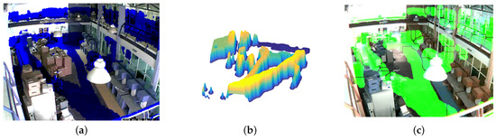
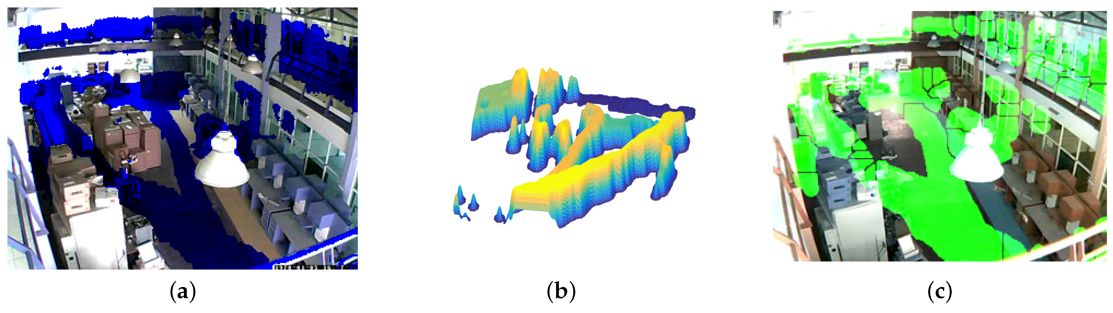
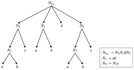
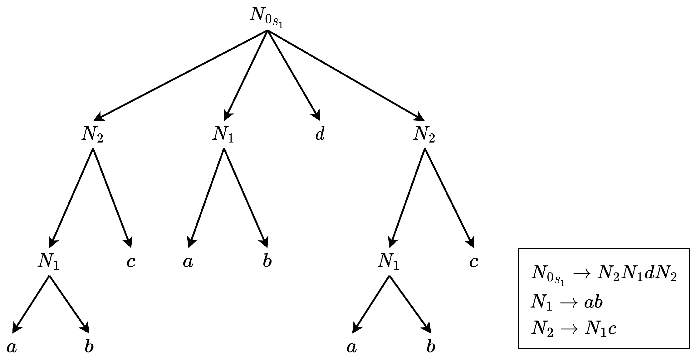
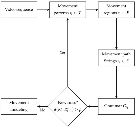
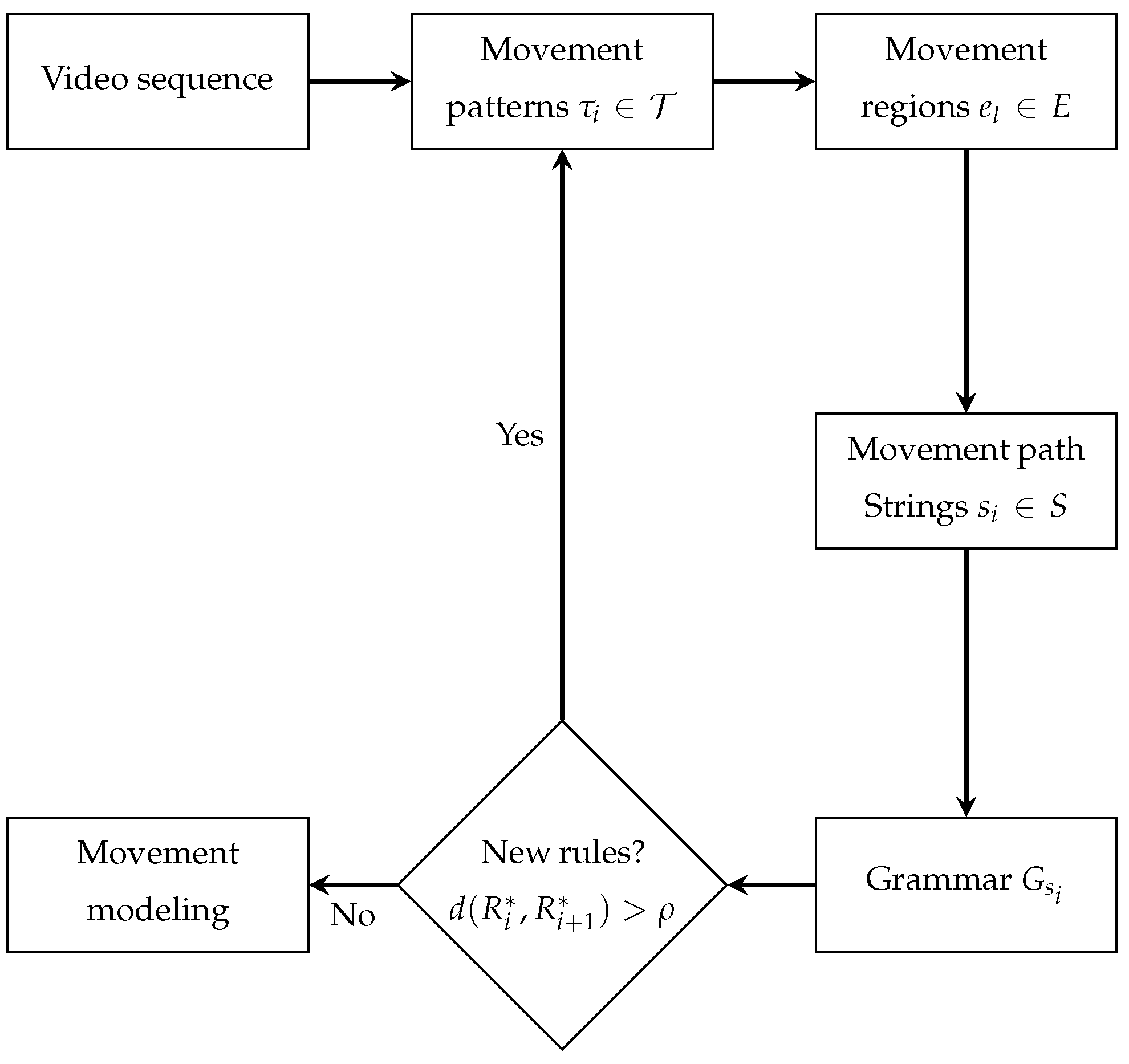
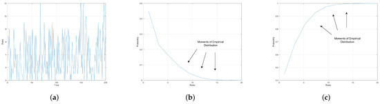
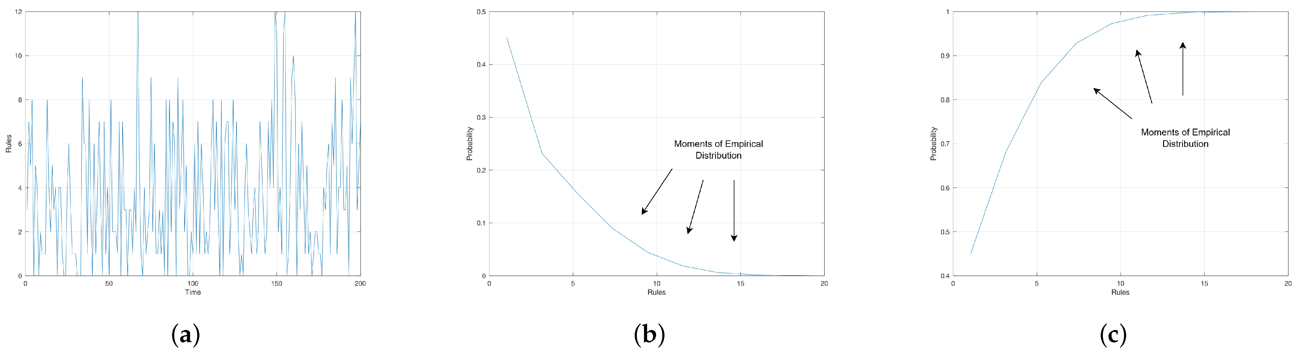
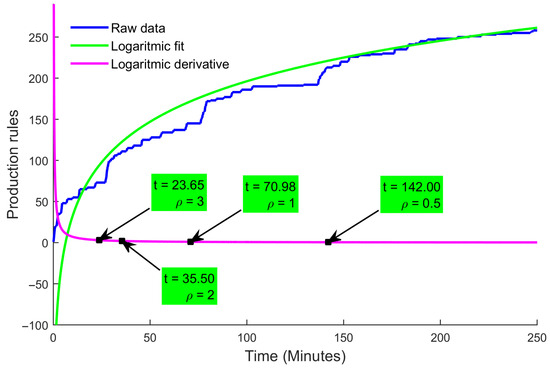
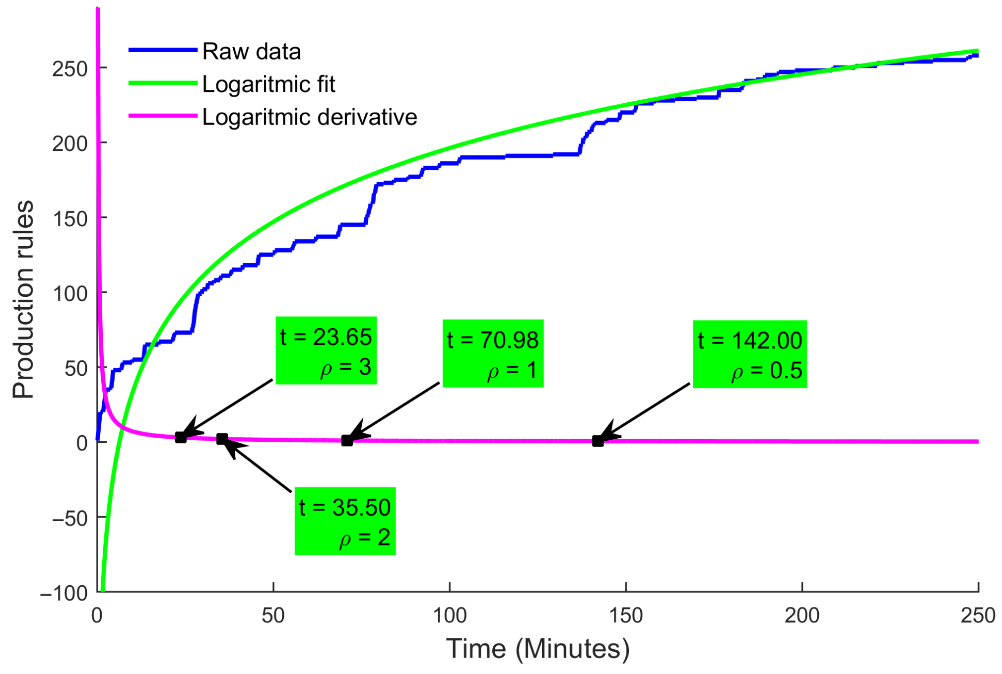
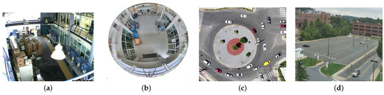
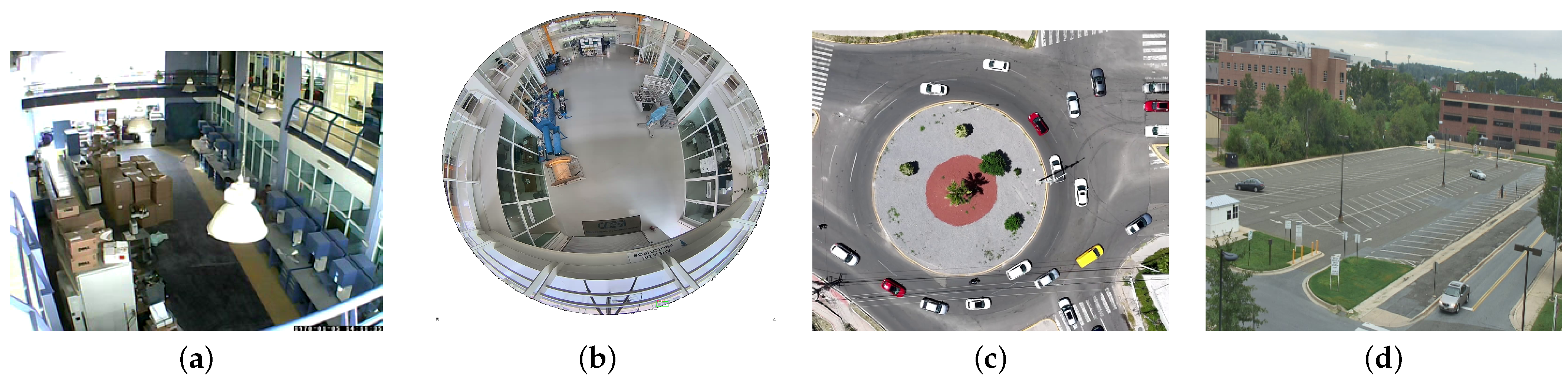


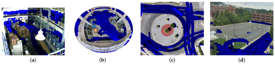
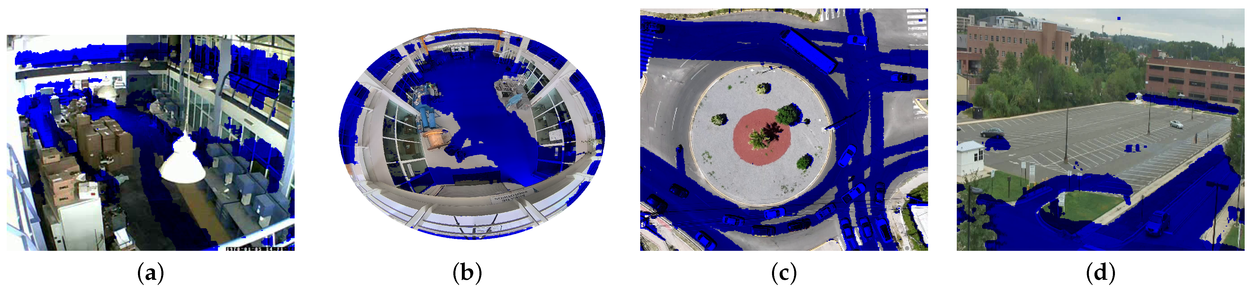
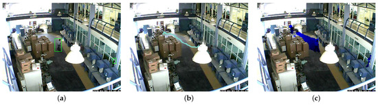
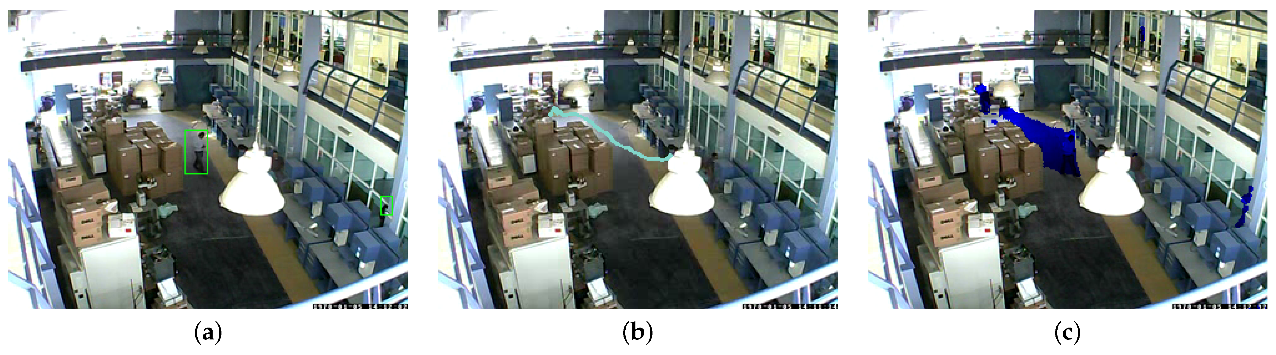
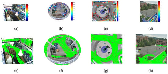
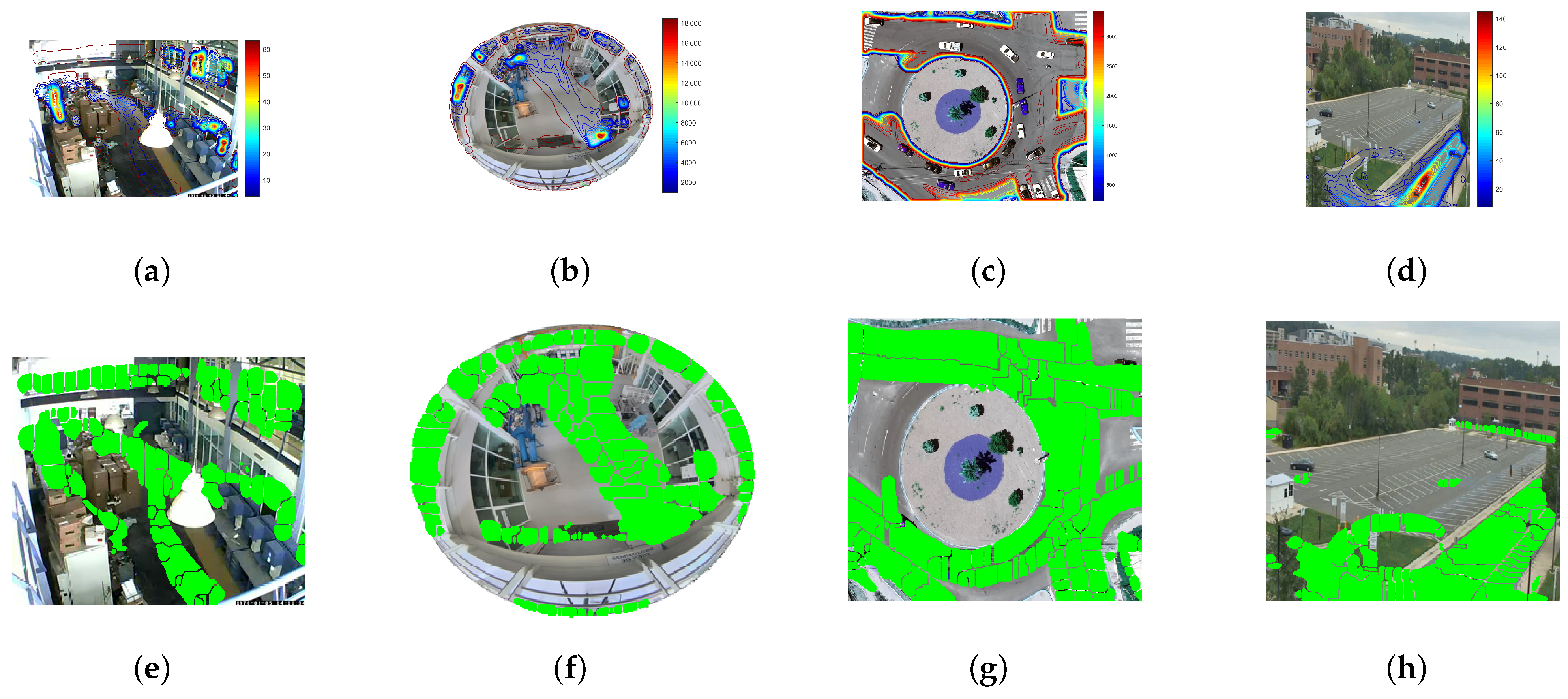
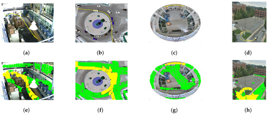
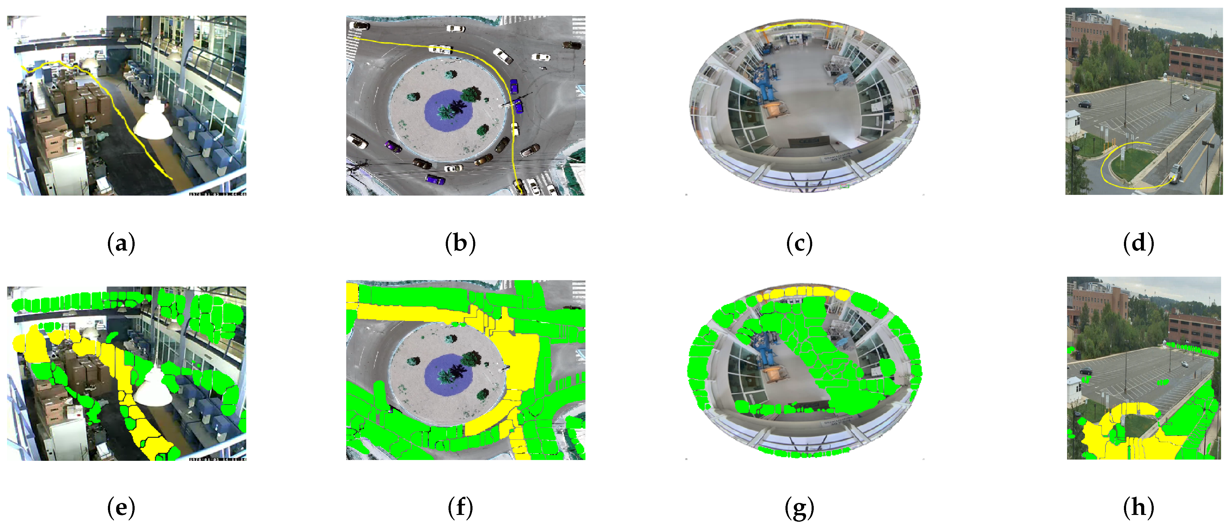
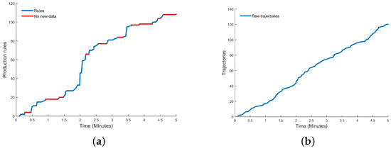
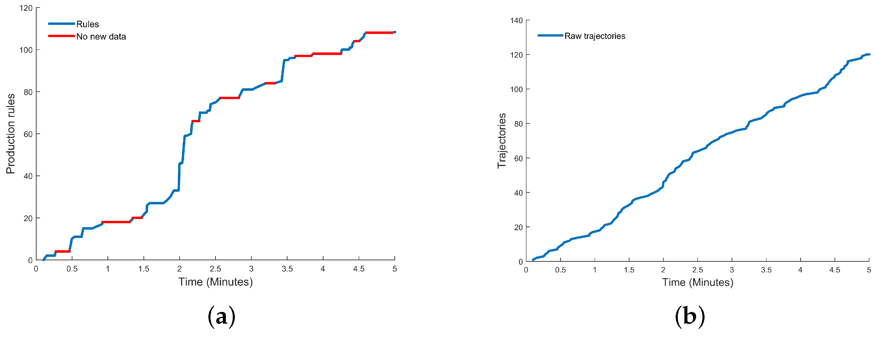
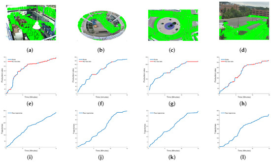
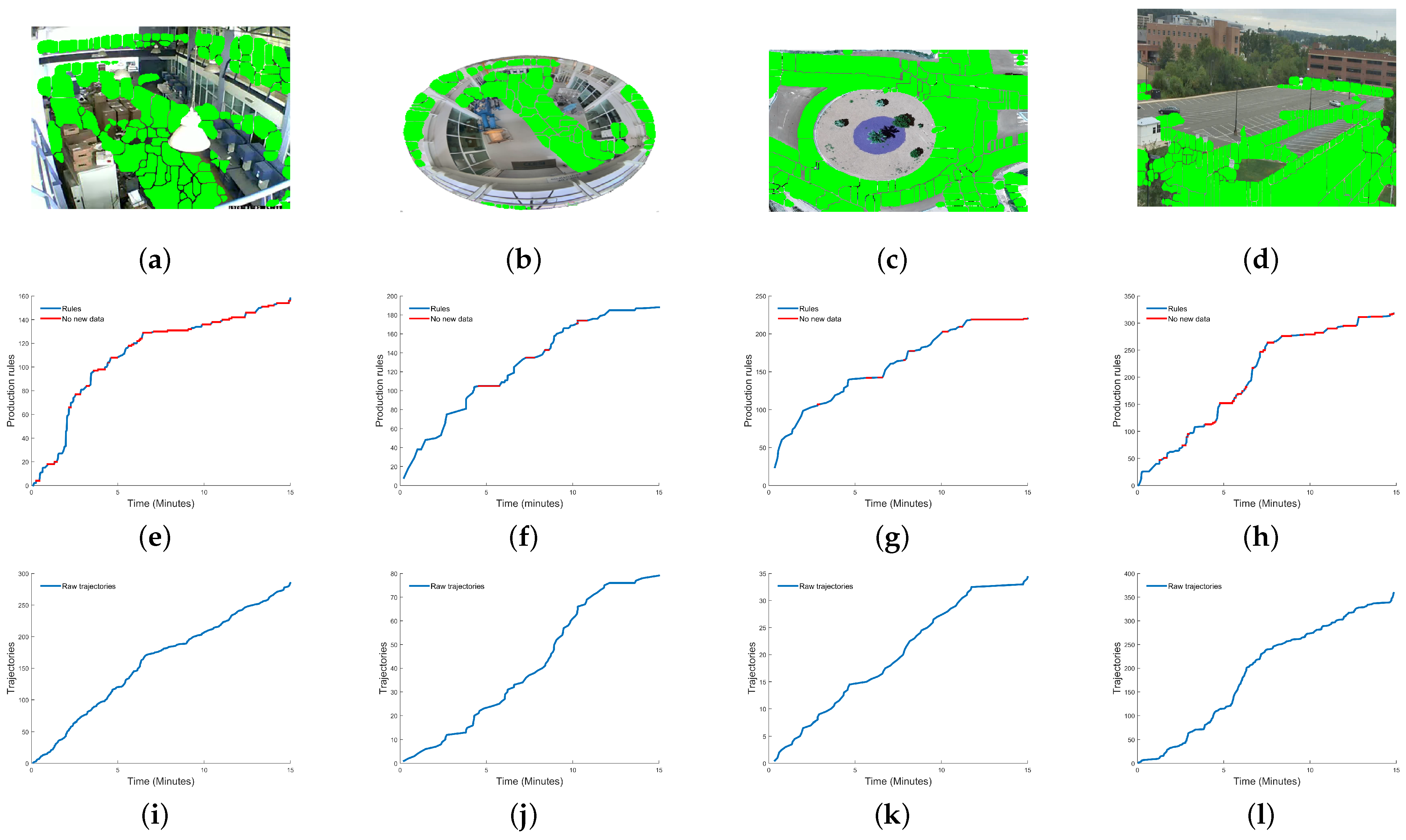
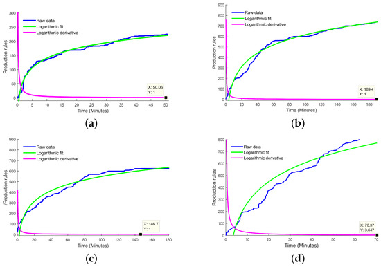
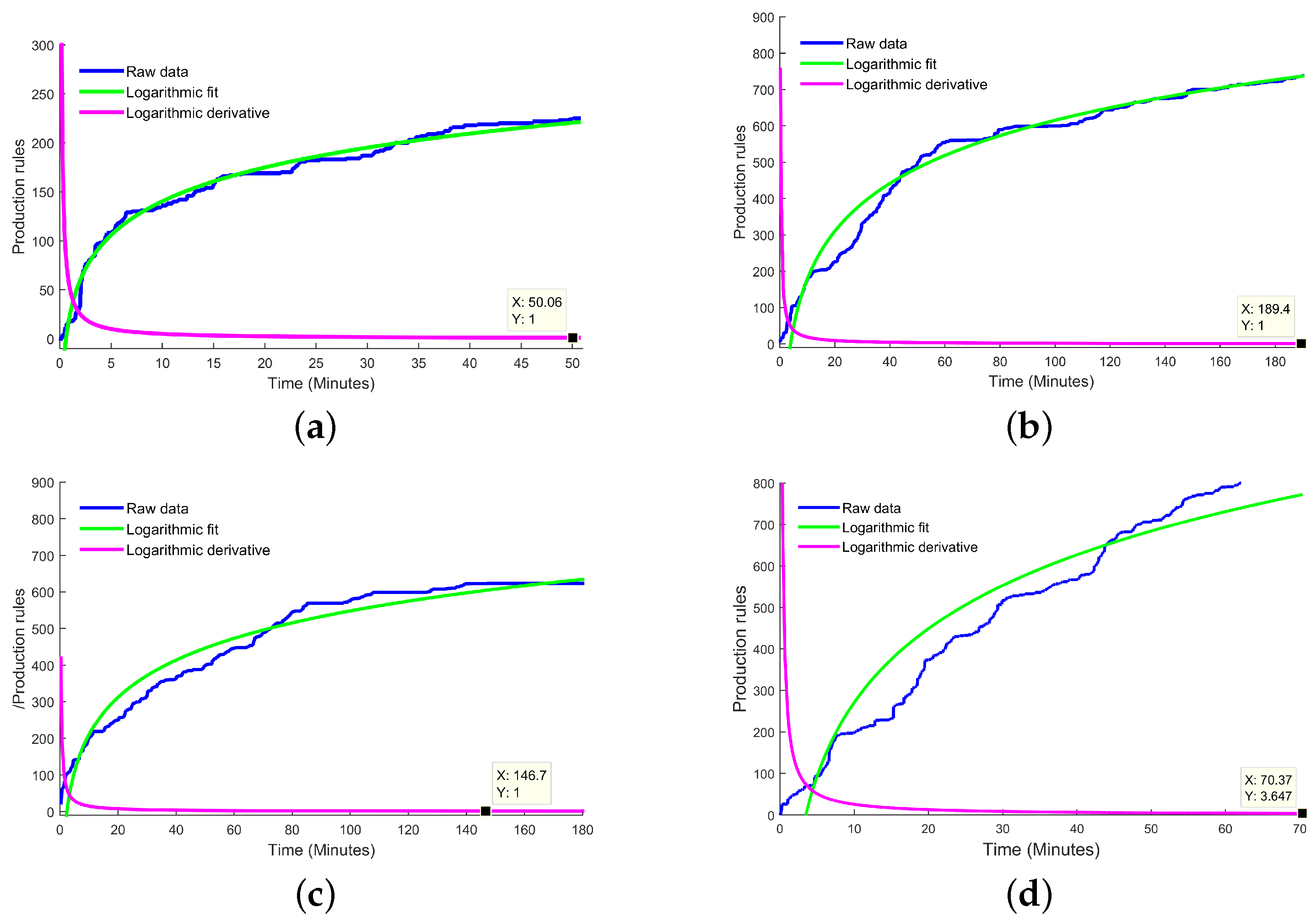
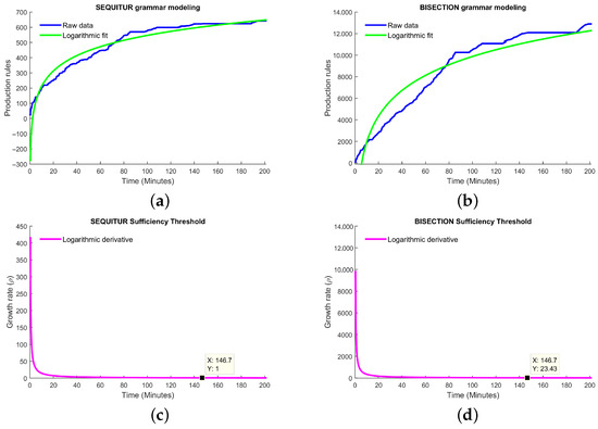
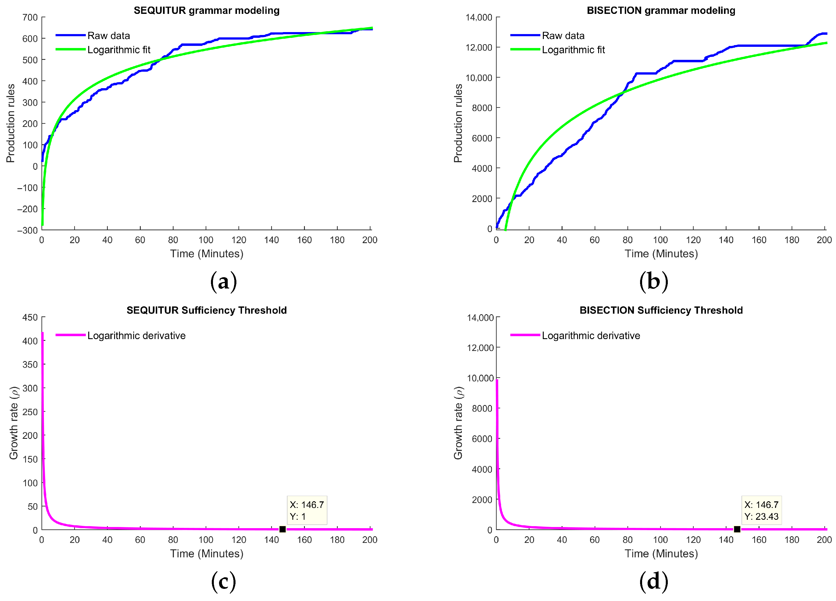
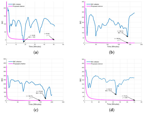
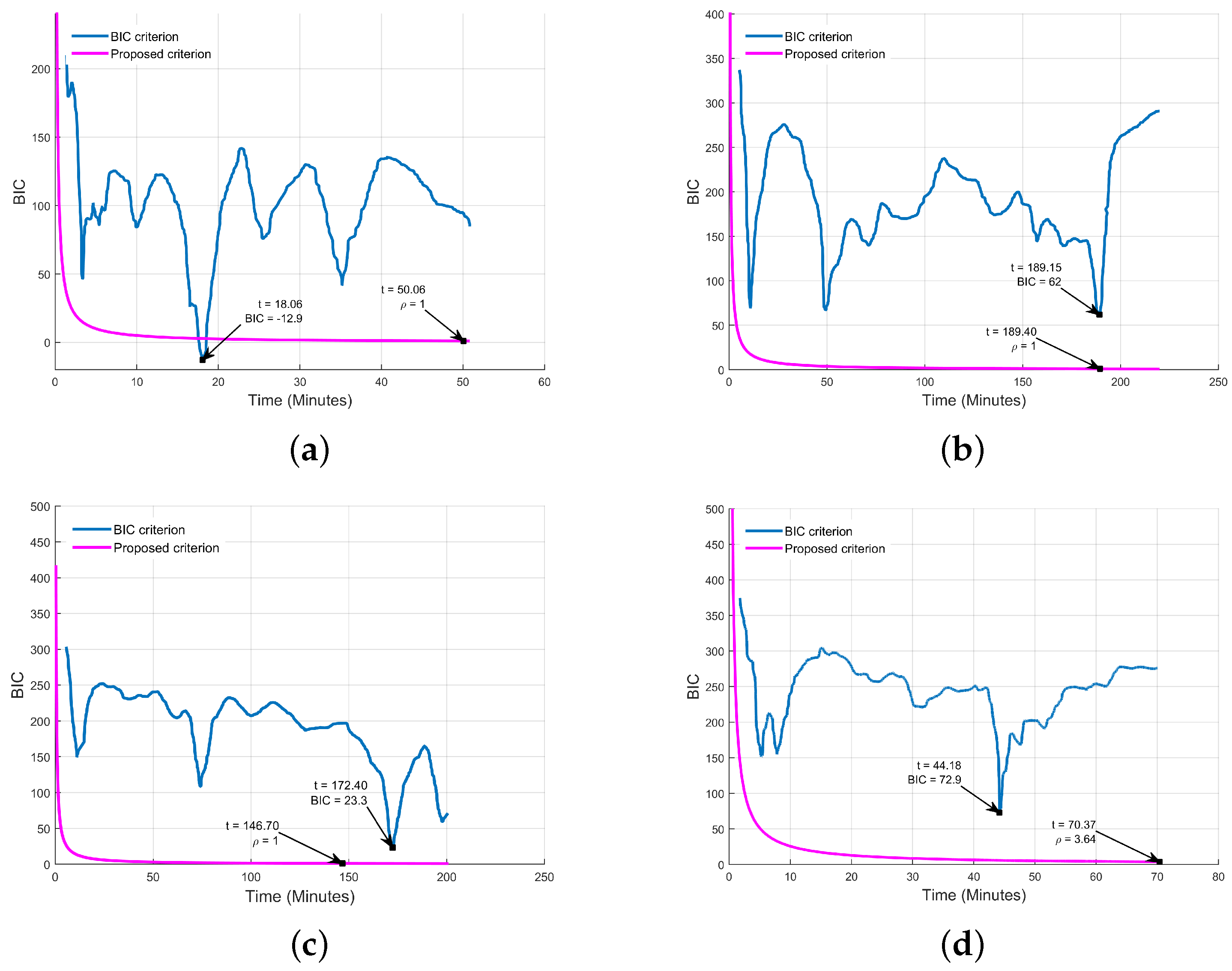
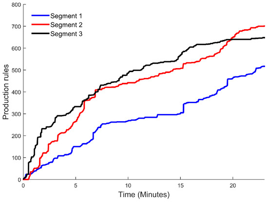
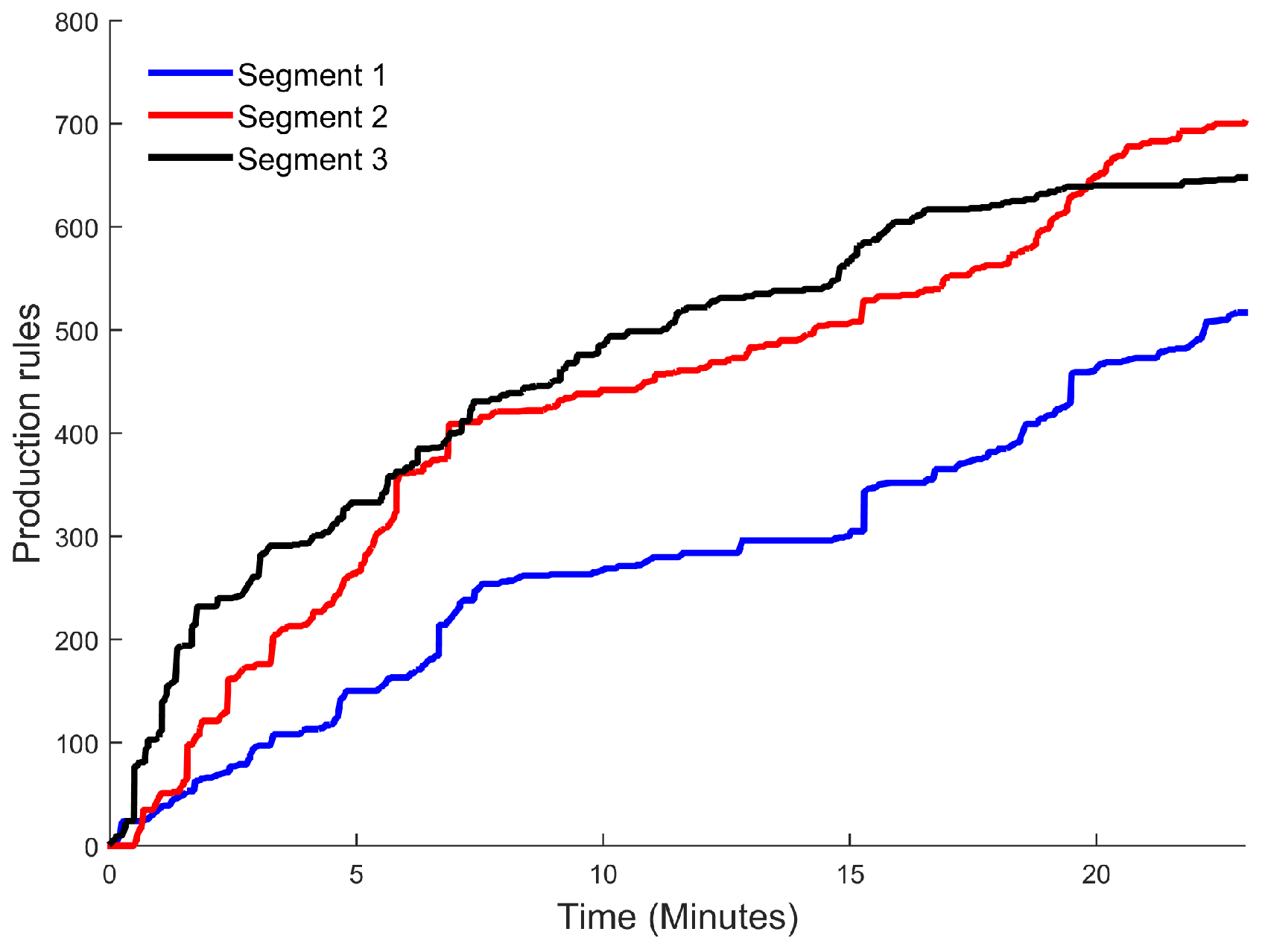
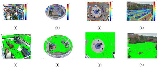
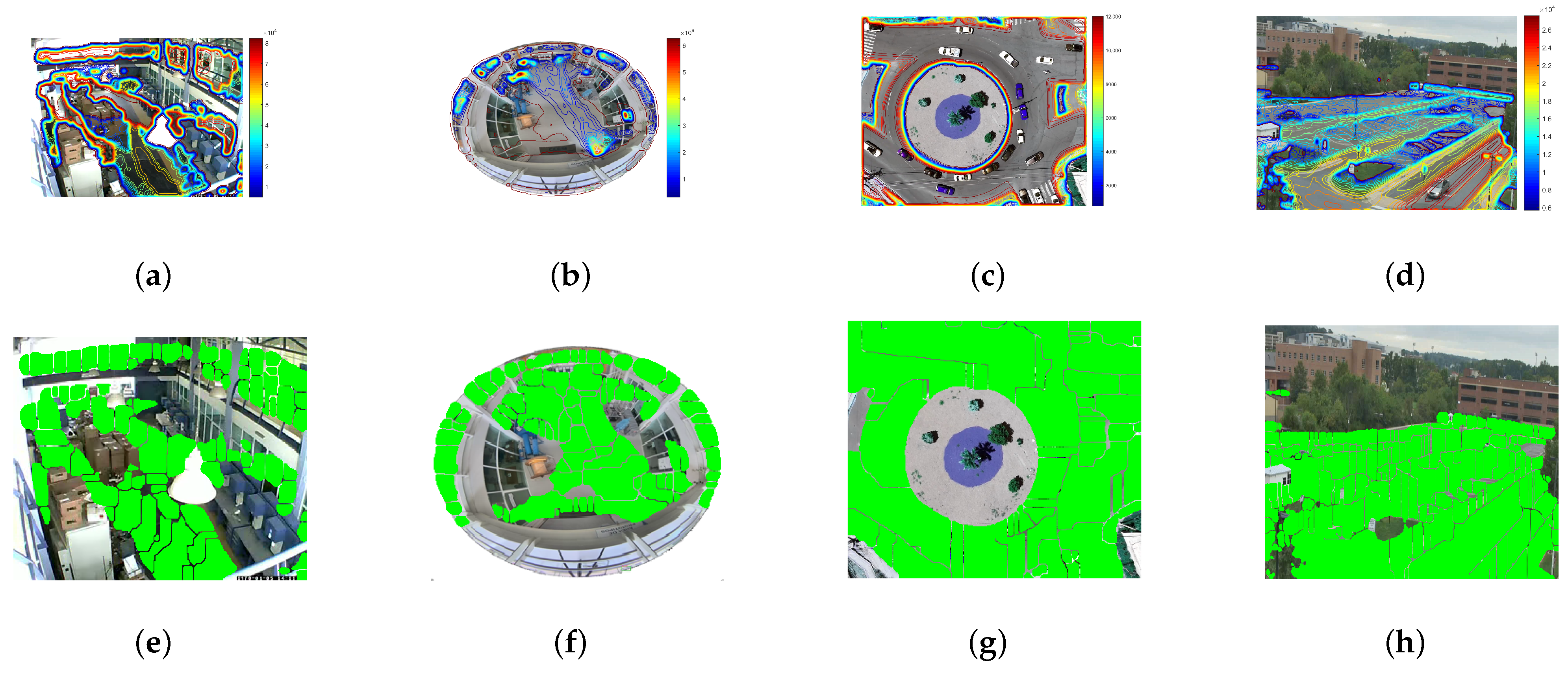
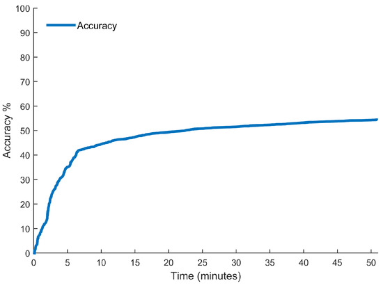
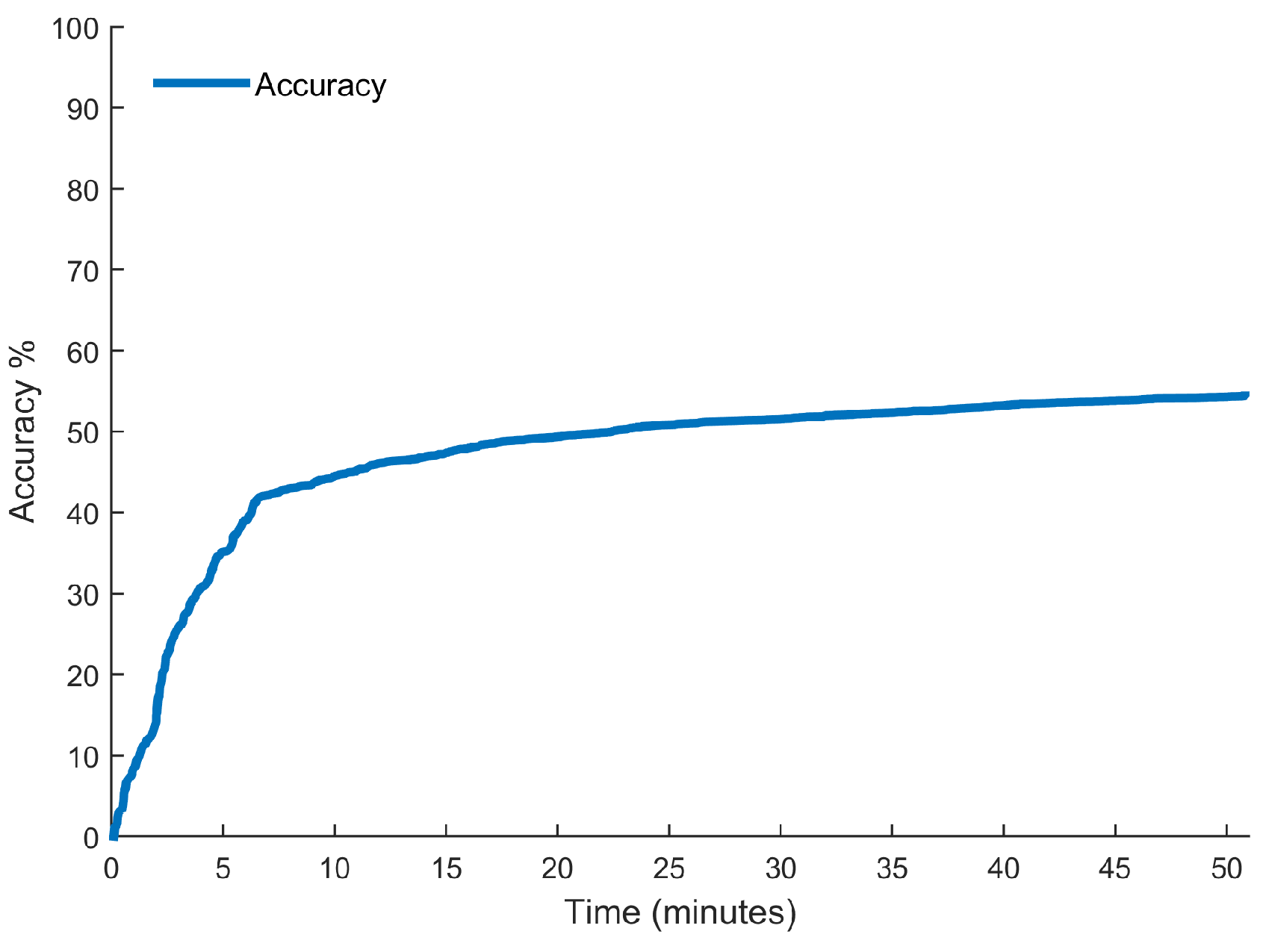

Disclaimer/Publisher’s Note: The statements, opinions and data contained in all publications are solely those of the individual author(s) and contributor(s) and not of MDPI and/or the editor(s). MDPI and/or the editor(s) disclaim responsibility for any injury to people or property resulting from any ideas, methods, instructions or products referred to in the content. |
© 2026 by the authors. Licensee MDPI, Basel, Switzerland. This article is an open access article distributed under the terms and conditions of the Creative Commons Attribution (CC BY) license.