Article

Modeling Global Warming from Agricultural CO2 Emissions: From Worldwide Patterns to the Case of Iran

by
Raziyeh Pourdarbani
1,*,
Sajad Sabzi
2,*,
Dorrin Sotoudeh
3,
Ruben Fernandez-Beltran
4,*,
Ginés García-Mateos
4 and
Mohammad Hossein Rohban
3
1
Department of Biosystems Engineering, University of Mohaghegh Ardabili, Ardabil 56199-11367, Iran
2
Department of Biosystems Engineering, Gorgan University of Agricultural Sciences and Natural Resources, Gorgan 49189-16573, Iran
3
Department of Computer Engineering, Sharif University of Technology, Tehran 14588-89694, Iran
4
Department of Computer Science and Systems, University of Murcia, 30100 Murcia, Spain
*
Authors to whom correspondence should be addressed.
Modelling 2025, 6(4), 153; https://doi.org/10.3390/modelling6040153
Submission received: 26 September 2025 / Revised: 11 November 2025 / Accepted: 17 November 2025 / Published: 24 November 2025
(This article belongs to the Section Modelling in Artificial Intelligence)

Abstract

Agriculture is a major source of greenhouse gas emissions, yet predicting temperature increases associated with specific CO2 sources remains challenging due to the heterogeneity of agri-environmental systems. In response, this study presents a machine learning framework that adopts an agri-food system boundary (production to retail) and combines systematic model benchmarking, interpretability, and a multi-scale perspective. Seven regression models, including tree ensembles and deep learning architectures, are evaluated on a harmonized dataset covering 236 countries over the 1990–2020 period to forecast annual temperature increases. Results show that gradient-boosted decision trees consistently outperform deep learning models in predictive accuracy and offer more stable feature attributions. Interpretability analysis reveals that spatio-temporal variables are the dominant drivers of global temperature variation, while environmental and sector-specific factors play more localized roles. A country-level case study on Iran illustrates how the framework captures national deviations from global patterns, highlighting intensive rice cultivation and on-farm energy use as key influential factors. By integrating high-performance predictions with interpretable insights, the proposed framework supports the design of both global and country-specific climate mitigation strategies.

Graphical Abstract

1. Introduction

Human-driven greenhouse gas (GHG) emissions are transforming the climate of the Earth more rapidly than at any other time since systematic measurements began [1]. The Sixth Assessment Report of the Intergovernmental Panel on Climate Change [2] attributes roughly 1.1 °C of the observed rise in global mean surface temperature to the cumulative burden of this type of gases. Their warming influence already reverberates throughout the climate system: glaciers retreat and ice sheets thin [3], mean sea level rises [4], and extremes in temperature and precipitation are becoming more intense and more frequent [5]. Within the GHG mix, carbon dioxide (CO2) stands out due to its sheer atmospheric abundance and its persistence, that is, once emitted, a fraction remains for centuries [6]. Although methane (CH4) and nitrous oxide (N2O) have a stronger warming potential per molecule, their shorter atmospheric lifetimes mean that the climate legacy of the present day CO2 emissions will continue with us long after the others have faded [7]. In other words, the CO2 we release today will define the climate that awaits future generations.
Against this global backdrop, the agricultural sector certainly occupies a pivotal position [8]. Agriculture, forestry and other land use form a critical node in the climate-carbon nexus, since they are a notable source of CO2 while simultaneously being highly vulnerable to shifts in temperature and water availability. Recent inventories estimate that agriculture alone contributes roughly 11–15% of total anthropogenic GHG output, surpassed only by electricity generation and transport on the global ledger [9]. Most agricultural CO2 comes from activities such as land conversion (e.g., deforestation for cropland, which releases stored carbon), diesel-powered field operations, energy-intensive irrigation pumping, and open burning of crop residues [10,11]. The continued warming and increasing hydroclimatic volatility threaten agricultural yields and rural livelihoods, creating a self-sustaining loop in which increasing exposure erodes the sector’s adaptive capacity while simultaneously amplifying its emissions footprint. These interconnected vulnerabilities underscore the urgent need for comprehensive analyses capable of modeling the complexity of agri-environmental systems, thus forming robust climate policies and improving the resilience of the agricultural sector under future climate scenarios [12].
Meeting these analytical needs in agri-environmental modeling depends critically on our ability to translate heterogeneous data sources, ranging from agri-environmental indicators to geospatial features, into accurate climate-relevant predictions. However, traditional modeling approaches often fall short in this regard. Inventory-based models provide retrospective estimates, but lack the capacity for forward-looking prediction [13]. Mechanistic simulators, such as crop or climate process models, represent biophysical complexity more faithfully, yet they demand extensive input data, are computationally intensive, and remain difficult to scale globally [14]. Simpler statistical methods, including linear regression models, offer interpretability but struggle to capture the nonlinear dynamics that characterize the climate-agriculture tandem. An illustrative example is provided by Murad et al. [15], who identified a significant bidirectional association between agricultural output and per capita CO2 emissions. However, the simplicity of the model and the limited availability of explanatory variables constrained its ability to reflect complex interactions. Taken together, these classical tools either oversimplify the problem or focus narrowly on mechanistic pathways, ultimately limiting their capacity to predict the spatial and temporal variability of CO2 emissions across diverse agricultural systems.
During the past decade, machine learning (ML) methods have transformed the way researchers study GHG emissions in agricultural contexts [16,17]. Early work in the mid-2010s relied on relatively simple shallow algorithms, such as decision trees, support vector machines (SVM), or single-layer neural networks, to demonstrate that data-driven predictive models could outperform linear regressions when there were nonlinear interactions between management, soil, and climate variables. For instance, Safa et al. provided one of the first proofs of concept with a feedforward artificial neural network (ANN) that predicted wheat crop emissions more accurately than a conventional linear benchmark [18]. In parallel, kernel-based support vector machines (SVM) were used to forecast sectoral CO2 emissions in China, while a Least Squares SVM approach incorporating economic structure and targeted feature selection further improved predictive accuracy [19]. Additionally, Pérez-Miñana et al. [20] explored Bayesian Networks for GHG management in British agriculture, showing that probabilistic modeling can improve transparency and stakeholder understanding by linking emissions directly to their economic cost. These first-generation studies validated the ML approach, but their performance was sometimes limited by small sample sizes and the inability to capture intricate dynamics.
As larger multi-site datasets became available, tree-based ensembles emerged as the workhorse for agricultural emission modeling. Random Forests (RF), which aggregate hundreds of bootstrapped decision trees, proved adept at modeling the cyclical and seasonal behavior of soil CO2 fluxes. Shiri et al. [21] applied a Random Forest model to estimate CO2 flux components across 11 forest sites, showing that temperature and radiation variables could drive accurate predictions even under data-scarce conditions. In larger multi-year compilations, gradient-boosted decision trees (GBDT) have consistently outperformed other methods. Adjuik and Davis [22], using the USDA GRACEnet database, found that a GBDT model delivered strong predictive performance on training data and matched RF as the top performer on unseen test data, ahead of SVM and k-nearest neighbors regressors. Wu et al. [23] extended this paradigm by using Extreme Gradient Boosting (XGBoost) to predict CH4 and N2O emissions from paddy fields in various management scenarios in China, obtaining robust precision and identifying key emission drivers through a feature importance analysis. Thanks to their ability to model complex interactions with modest data volumes and their built-in variable importance scores, RF and GBDT became some of the most popular baselines in agricultural emission modeling and related environmental applications.
The latest phase in this methodological evolution is marked by deep feed-forward neural networks, which can rival, and occasionally surpass, ensemble trees when the feature space is rich enough. Harsanyi et al. [24] benchmarked gradient boosting, SVM and two deep architectures, a fully connected neural network (FNN) and a convolutional neural net (CNN), on maize-field fluxes across two distinct climatic regions. The FNN achieved the highest test accuracy, with gradient boosting performing similarly well. Xue [25] leveraged a neural network based on radial basis functions to predict soil CO2 fluxes from key soil and climate variables during crop growth, demonstrating superior performance over linear models and standard feedforward networks in capturing nonlinear emission patterns. In [26], Wang et al. introduced a multi-scale deep learning framework combining attention-based encoders for daily and monthly CO2 data. Their model was able to reach state-of-the-art performance in long-term atmospheric CO2 forecasting, outperforming several baselines at a reasonable computational cost. Although these and other recent deep learning approaches show competitive results, particularly in settings with dense temporal data [27], many global emission inventories collected over extended periods lack a strong spatial or sequential structure. This limits the suitability of convolutional or sequence-based models. Instead, models tailored to tabular data, such as the Network on Network (NON) architecture [28], offer a compelling alternative by learning dedicated feature embeddings.
As modern ML models increasingly outperform traditional approaches in predicting agricultural CO2 emissions, their lack of interpretability often becomes a critical barrier to real-world adoption, especially in policy contexts that demand transparency and justification of model outputs. Tree-based methods partially address this challenge through their built-in variable importance metrics, offering a degree of interpretability by design. However, deep learning architectures operate as black boxes, making it difficult to trace individual predictions back to meaningful drivers. In this context, explainable artificial intelligence (XAI) techniques have emerged as a powerful tool to bridge the gap between performance and transparency. These techniques are applied after model training and aim to interpret how input variables influence the resulting predictions, thereby identifying the most relevant factors behind the model’s behavior. Rather than modifying the model itself, they provide an additional analytical layer that enhances transparency and facilitates trust in data-driven conclusions. Among them, the SHAP (SHapley Additive exPlanations) framework [29] builds on the Shapley value concept from cooperative game theory, in which each feature is regarded as a ’player’ contributing to the overall model output. This theoretical basis allows SHAP to fairly quantify how much each variable contributes to a given prediction. This framework provides consistent, model-agnostic, and locally accurate attributions for both ensemble and neural models. Recent applications have demonstrated its effectiveness in climate-related modeling tasks. For instance, this approach has been used to validate the Environmental Kuznets Curve hypothesis [30] by revealing nonlinear relationships between income per capita and CO2 emissions [31]. In the transportation sector, it has also been applied to identify the main factors influencing vehicle CO2 emissions in Canada, such as urban and highway fuel consumption and fuel type, offering valuable insights for decarbonization strategies [32]. By translating complex model outputs into actionable information, this explainability method fosters stakeholder trust and facilitates the integration of ML into evidence-based climate policy.
Despite the clear benefits of capturing global patterns with XAI, climate mitigation decisions are ultimately formulated and implemented at the national level. Country-specific agro-ecological conditions, policy environments, and data-reporting practices can lead to substantial deviations from global emission patterns. For example, spatial optimization models show that low-emission strategies optimized globally may differ from those based on local sourcing, highlighting how efficiency and emissions vary regionally [33]. As a result, predictive frameworks must be flexible enough to accommodate local particularities without losing their generalization. Comparing global and country-level feature attributions then becomes essential not just to identify general and local drivers, but also to understand how global patterns translate into specific national contexts. This contrast can reveal the adaptability of predictive models to diverse conditions, reinforcing their utility for designing evidence-based mitigation policies that are both globally informed and locally actionable [34].
In response to these demands, this study develops a methodological framework to estimate surface temperature increases driven by agriculture-related CO2 emissions. The framework integrates systematic model benchmarking with explainable techniques and a multi-scale perspective, enabling robust global analysis while preserving relevance for country-level policy design. Three key challenges motivate the research conducted in this work. First, it remains unclear which type of ML model offers the best combination of robustness and accuracy when applied to medium-sized tabular datasets that integrate agri-environmental information. Existing research, for example [16,17,24], still provides limited findings on the specific task of predicting surface temperatures from agricultural CO2 emissions. Second, although many high-capacity models achieve excellent predictive performance, their inner workings are often opaque. This lack of interpretability complicates their use in policy-oriented settings, where decision-makers require not only accurate forecasts but also a clear understanding of the underlying drivers. Third, most global modeling approaches generalize across regions, frequently at the cost of overlooking country-specific dynamics. As a result, they struggle to support locally relevant mitigation strategies, particularly in countries with atypical emission profiles or distinct agro-environmental constraints.
To address these challenges in a specific data-driven setting, this work relies on a harmonized global dataset covering 236 countries over the period 1990–2020. This panel combines agriculture-related CO2 emissions with environmental, demographic, and geographic variables, offering a suitable basis for benchmarking ML models on structured, medium-scale data. To assess the capacity of the framework to generate actionable country-level insights, we complement the global analysis with a case study of Iran. This country exemplifies the complex interplay of agro-climatic stress, technological inertia, and institutional constraints. Its semi-arid climate, heavy reliance on groundwater irrigation, and high agricultural carbon intensity create a highly nonlinear emission profile that global patterns alone fail to resolve. Previous work on Iran’s agricultural emissions, such as Shabani et al. [35], focused on improving CO2 forecasts, but did not examine the role of temperature or provide interpretable insights between global and local patterns. Our framework addresses both gaps by explicitly modeling temperature effects and emphasizing explainability. As such, Iran serves as a critical case for testing the interpretability of the framework and its relevance in policy under national conditions. Overall, this study addresses the scientific problem of how to accurately model and interpret agriculture-related CO2 emissions and their temperature impacts in a way that combines predictive performance, interpretability, and multi-scale relevance. Building on this context, the paper makes four main contributions:
  • A systematic benchmarking protocol that compares seven machine learning regression models on the specific task of linking agricultural CO2 emissions to surface temperature changes, under a unified preprocessing, tuning, and validation setup.
  • An interpretability scheme that combines impurity-based importance metrics with model-agnostic SHAP analyses to provide transparent, multi-scale explanations of emission drivers.
  • Empirical evidence, in our dataset, that gradient-boosted tree models consistently outperform deep tabular networks on medium-sized agri-environmental data, while providing more stable feature attributions.
  • A multi-scale application contrasting global feature attributions with a national case study (Iran), showing how the same methodological pipeline can support both international benchmarking and country-level mitigation analysis.
The remainder of the paper is structured as follows. Section 2 describes the dataset, the regression models considered, and the interpretability tools used in the study. Section 3 presents the experimental results, including a comparative performance evaluation of all models, a multi-model interpretability analysis, and a case study on Iran. Finally, Section 4 summarizes the main findings, discusses their implications for environmental modeling and policy, and outlines directions for future work.

2. Materials and Methods

2.1. Dataset Description

The dataset used in this work is based on the Agri-food CO2 emission dataset—Forecasting ML, published by Alessandro Lo Bello on Kaggle [36]. It comprises annual records from 236 countries covering the period from 1990 to 2020, totaling over 7000 instances. Each record includes environmental, agricultural, and demographic variables, along with the target variable of this study: the increase in temperature at the country level. The collection originally comprised 31 features spanning various GHG emissions sources (e.g., ‘Savanna Fires’, ‘Crop Residues’, ‘Rice Cultivation’, ‘Manure Management’, etc.), socio-economic indicators (‘Urban Population’, ‘Rural Population’, ‘Food Transport’), aggregate measures such as total emissions, and the annual average temperature increase (‘Average Temperature’). It is important to note that this dataset covers the entire agri-food system, including downstream emissions from transport, retail, and waste, not just on-farm agricultural production. A complete description of all variables and units is provided in Table 1.
To enrich the data with geographical context, we introduced some additional features: ‘continent’, ‘latitude’, ‘longitude’, and ‘altitude’. Geographic covariates were obtained from open public sources: country coordinates [37] (providing ‘latitude’ and ‘longitude’) and average country elevation [38] (providing ‘altitude’). While [38] is an aggregator, this specific data (average elevation) is static, factual, and has been verified as consistent with other public geographical repositories.
In addition, several preprocessing steps were applied to ensure data quality and model compatibility. Initially, inconsistent features were removed. The columns ‘Total Population-Male’ and ‘Total Population-Female’ were excluded due to discrepancies with the population figures based on urban and rural areas. Then, a new ‘Total Population’ feature was computed, and the values of ‘Urban Population’ and ‘Rural Population’ were normalized with respect to this total, in order to represent relative demographic distributions. Subsequently, additional preprocessing was performed to prepare the data for model training. Categorical variables such as ‘continent’ were encoded either ordinally or through one-hot vectors depending on the requirements of each model. Missing values were also imputed using feature-wise means, and duplicate entries were removed from the collection. Moreover, the column containing country information was discarded to eliminate redundancy, given the inclusion of more informative spatial features.
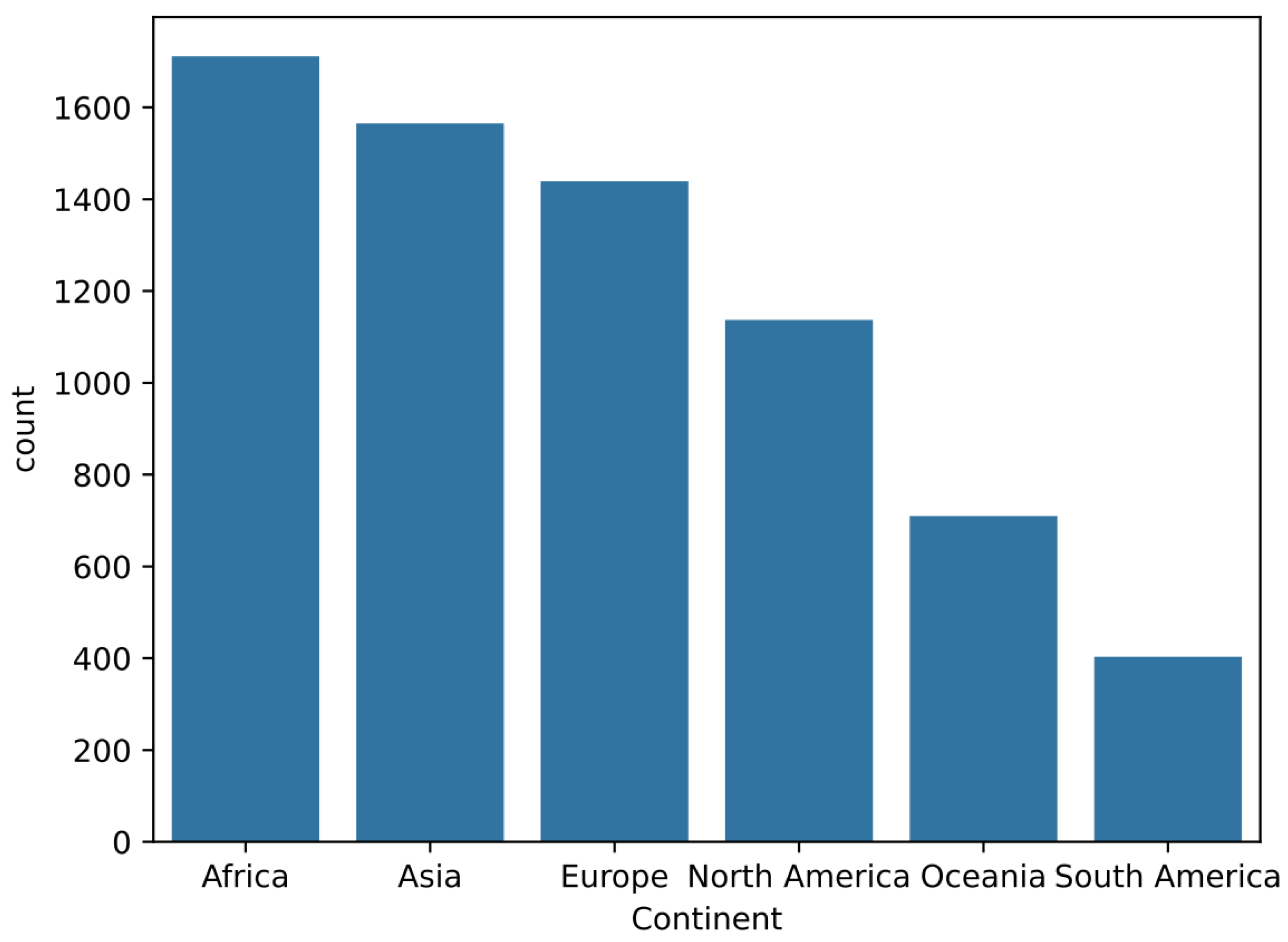
The resulting data were then divided into training (70%), validation (15%), and test (15%) splits, using stratified sampling based on the ‘continent’ feature in order to preserve the geographic distribution. As Figure 1 shows, the dataset presents a significant imbalance across continents. To ensure representative learning and prevent geographic bias, this distribution was proportionally preserved across the training, validation, and test splits. In order to reduce multicollinearity, features with a Pearson correlation coefficient greater than 0.95 were removed following an analysis of the correlation matrix computed on the training set. Finally, all continuous features were standardized using the mean and standard deviation calculated from the training data.
Conceptually, the dataset can be viewed as a single large table (or matrix), where each row corresponds to a specific country in a specific year (e.g., ‘Iran, 1995’), and each column corresponds to one of the variables listed in Table 1. Among these variables, ‘Average Temperature’ serves as the target attribute of the study.
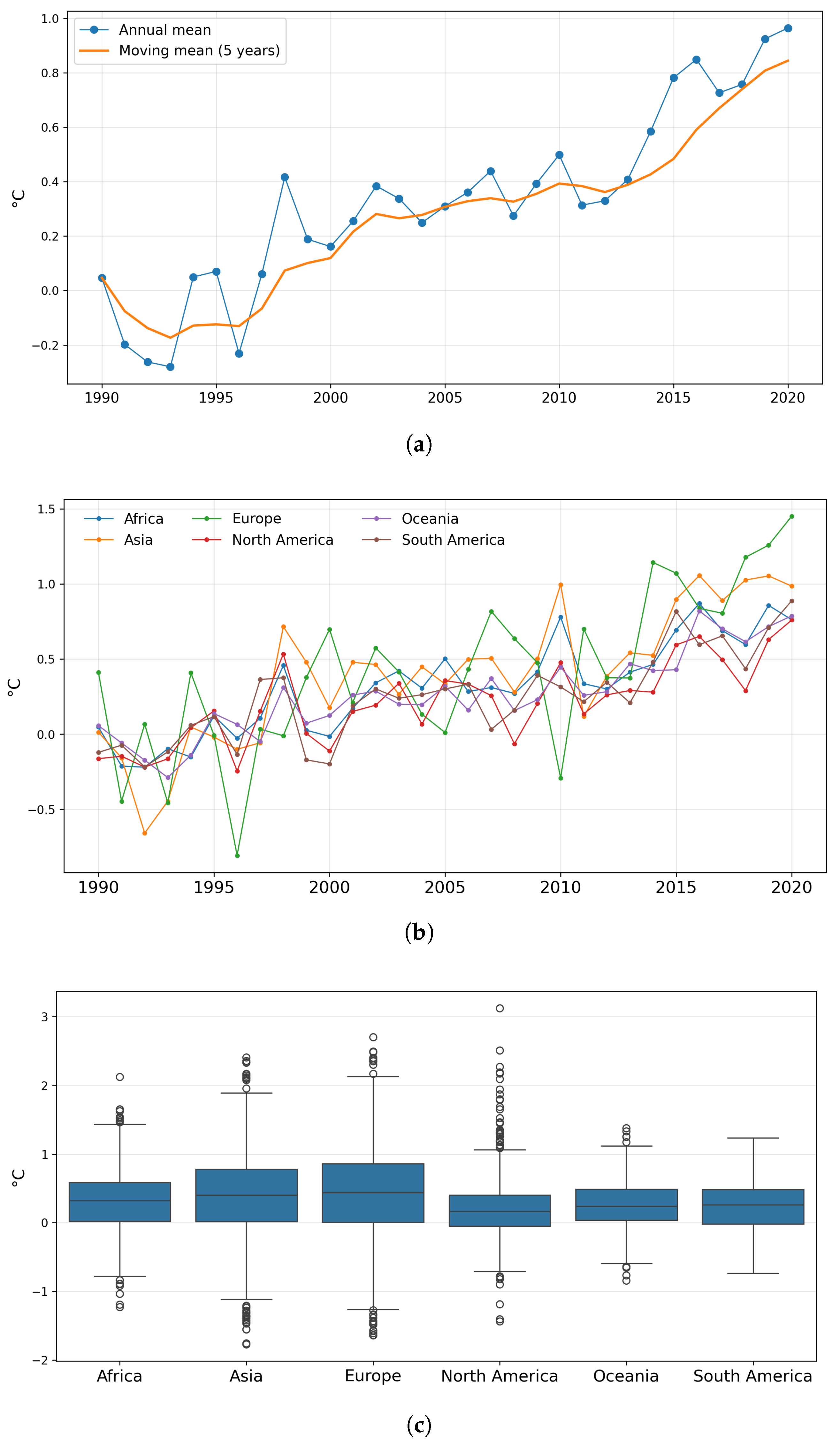
To illustrate the complexity of the target variable, ‘Average Temperature’, and to motivate the necessity for advanced regression models, a preliminary exploratory analysis was conducted. Figure 2 presents several views of the temperature data from 1990 to 2020.
As shown in Figure 2a, the global mean temperature exhibits a clear and accelerating upward trend, with the 5-year moving average smoothing out high annual volatility. However, this global trend masks significant regional heterogeneity. Figure 2b breaks down the mean temperature by continent, revealing distinct patterns and varying degrees of volatility. Europe, for instance, shows a much steeper and more erratic increase compared to other continents. This high variability between geographic regions is further confirmed by the temperature distributions shown in Figure 2c, where differences in medians, interquartile ranges, and outlier presence are evident across continents.
Taken together, these visualizations demonstrate that the target variable is characterized by: (i) a strong, non-stationary global trend, (ii) high spatio-temporal heterogeneity and variance, and (iii) complex, non-linear relationships that differ by region. A simple global model would fail to capture this intricate behavior, thereby justifying the benchmarking of sophisticated, data-driven machine learning models capable of learning these multi-scale patterns.

2.2. Regression Methodology

To effectively model the complex relationship between CO2 emissions and global temperature rise, we selected a diverse set of regression algorithms that are well suited for structured and heterogeneous data. The benchmark includes seven models in total: five ensemble algorithms that aggregate multiple decision trees and two neural network models. On the one hand, the ensemble methods include Random Forests, Gradient Boosting Machines, Extreme Gradient Boosting (XGBoost), Light Gradient Boosting Machine (LightGBM), and Gradient Based Decision Tree Ensembles (GRANDE). On the other hand, the neural network models cover the Multilayer Perceptron (MLP) and the Network on Network architecture (NON). The ensembles contribute robustness, resistance to overfitting, and clear estimates of variable importance, whereas the neural networks add capacity to learn subtle nonlinear interactions. Together, these methods provide both the predictive power needed to describe intricate emission patterns and the transparency essential for a sound climate assessment.
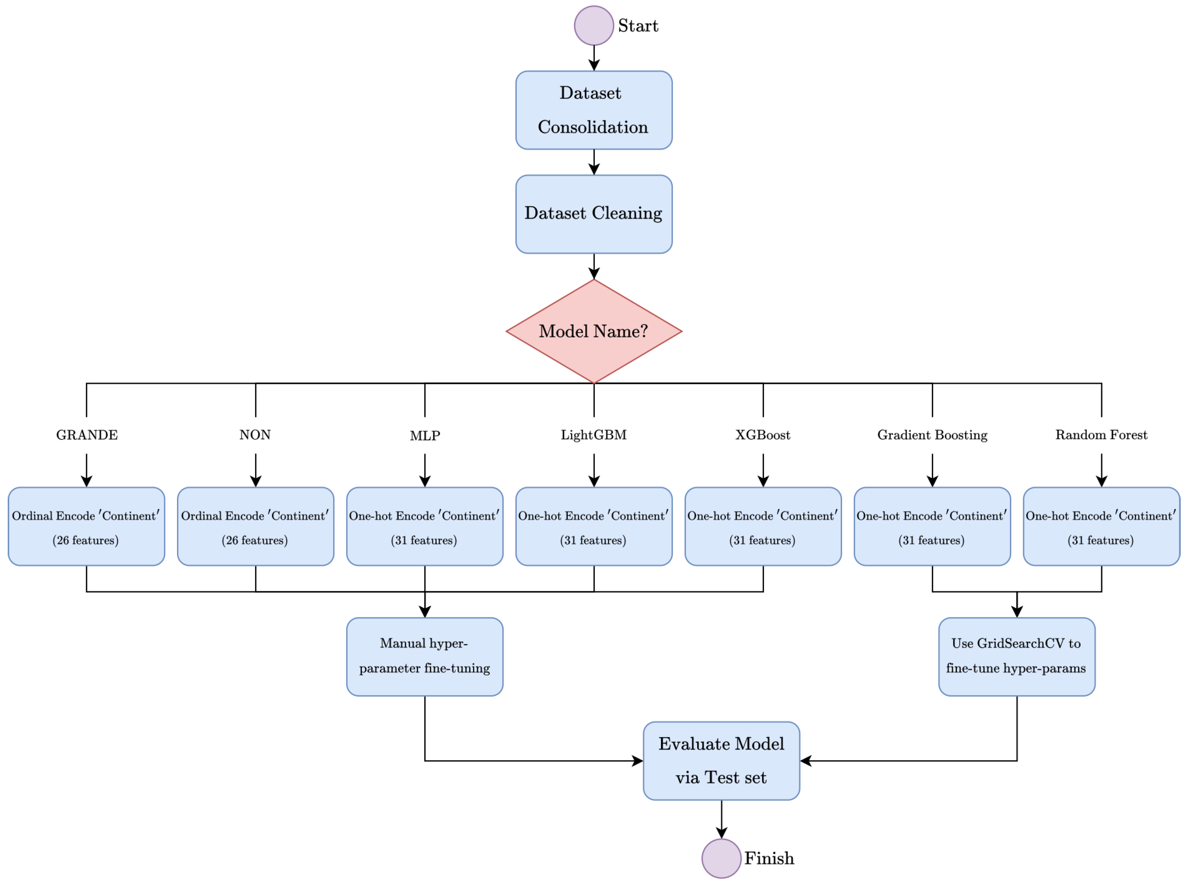
The general workflow of the regression methodology is depicted in Figure 3. After the initial dataset consolidation and cleaning steps (Section 2.1), model-specific handling of the ‘continent’ feature was performed: ordinal encoding (26 features) for GRANDE and NON, and one-hot encoding (31 features) for MLP, LightGBM, XGBoost, Gradient Boosting, and Random Forest. As is possible to see, hyperparameter optimization strategies also varied, employing GridSearchCV with 5-fold cross-validation on the training set for Random Forest and Gradient Boosting, and manual tuning on the validation set (typically with early stopping) for the remaining models. The final generalization performance of each optimized model was then assessed on the held-out test set.
The following subsections describe each regression method considered in this study, along with its specific configuration and training strategy. Each model is trained to predict the annual increase in surface temperature from the structured input features. Throughout this section, we denote the input vector by x, the corresponding true temperature increase by y, and the model prediction by y ^ .

2.2.1. Random Forest

Random Forest [39] is an ensemble learning algorithm widely used for regression and classification tasks due to its robustness against overfitting and strong performance on tabular data [40]. It mainly operates by constructing a multitude of decision trees, each built using a bootstrap sample (random sampling with replacement) of the training data. Crucially, Random Forest introduces further randomness by selecting only a random subset of features for consideration at each potential split within a tree. For regression tasks, the quality of each split is determined by an impurity-based criterion, specifically the reduction in the sum of squared errors (SSE), also known as the squared error reduction rule (SERR), and the final prediction is obtained by averaging the predictions of all individual trees in the forest. This aggregation process can be formally expressed as
y ^ ( x ) = 1 B b = 1 B T b ( x ; Θ b )
where B is the number of trees, and T b ( x ; Θ b ) is the prediction of the b-th tree for input x. This ensemble averaging significantly reduces variance compared to a single decision tree, leading to more stable and accurate predictions.
To optimize the Random Forest regressor for predicting annual temperature increase, we applied GridSearchCV with 5-fold cross-validation on the training set. The search was carried out to maximize the coefficient of determination (R2) while exploring three key hyperparameters that govern model complexity and the size of the ensemble. As an impurity measure, we used the standard squared error criterion, also known as mean squared error (MSE). The best configuration obtained was n_estimators = 250, max_depth = 15, and min_samples_split = 10. Using 250 trees improves stability and reduces variance, limiting depth to 15 levels avoids overly complex trees, and requiring at least 10 samples per split prevents the model from fitting the noise present in small subsets.

2.2.2. Gradient Boosting

Gradient Boosting [41] is an ensemble technique that builds a predictive model sequentially in stages. Unlike Random Forest, where all trees are trained independently, Gradient Boosting adds one decision tree at each iteration to correct the residual errors of the current ensemble. Let us assume that after ( m 1 ) iterations the ensemble prediction is
F m 1 ( x ) = j = 1 m 1 η T j ( x ; Θ j ) ,
where T j ( x ; Θ j ) denotes the j-th tree with parameters Θ j . At iteration m a new tree T m ( x ; Θ m ) is fitted to the pseudo-residuals, that is, the negative gradient of the chosen loss with respect to F m 1 ( x ) , and the ensemble is updated by
F m ( x ) = F m 1 ( x ) + η T m ( x ; Θ m )
where η ( 0 , 1 ] is the learning rate (or shrinkage factor) that scales the contribution of the new tree. Under this scheme, the number of boosting iterations controls the total number of trees, and vice versa. Accordingly, the final prediction for an input x is given by the output of the ensemble after M rounds, that is, y ^ ( x ) = F M ( x ) . Because each tree has been optimized to reduce the residual error, Gradient Boosting often achieves very high accuracy, but its sequential dependence also makes it more susceptible to overfitting, necessitating regularization through shallow trees, small η , early stopping, or additional constraints.
To tailor the Gradient Boosting regressor for our experiments, we used the aforementioned GridSearchCV procedure with 5-fold cross-validation, using the MSE function to compute the residuals. In this case, the optimal parameters were identified as n_estimators = 100, learning_rate = 0.1, and max_depth = 8. Limiting the number of trees to 100 prevents Gradient Boosting from overfitting in the early stages, while allowing the bias to be incrementally reduced. In addition, individual trees can be simplified to a depth of 8 since each tree sequentially focuses on modeling the remaining error (pseudo-residual) between the true annual temperature increase and the prediction made by the current ensemble.

2.2.3. Extreme Gradient Boosting

Extreme Gradient Boosting (XGBoost) [42] is an optimized implementation of gradient boosting that delivers both high accuracy and efficiency on large-scale tabular datasets. XGBoost enhances the classical boosting framework with explicit 1 and 2 regularization on leaf weights, parallelized tree construction, and support for early stopping to prevent overfitting. It offers two split-finding algorithms: (i) the exact method, which evaluates all candidate split points, and (ii) the approximate (histogram) method, which bins feature values for faster search. It also incorporates sparsity-aware learning and out-of-core computation for memory-limited environments. These innovations allow XGBoost to scale seamlessly to millions of samples while maintaining state-of-the-art predictive performance.
To adapt the model to our temperature-prediction task, we trained the XGBoost regressor for up to 50,000 boosting rounds, with early stopping after 1000 rounds without improvement in the validation R2 score (see Section 2.3.3 for details on this metric). The objective was set to minimize the MSE between predicted and true values. We fixed the learning rate at 0.01 to ensure gradual stable updates, and set lambda ( 2 regularization) to 1 and alpha ( 1 regularization) to 0. We also used the ‘hist’ tree method with max_bin = 256 for efficient split finding, a ‘depthwise’ grow policy to expand splits closest to the root first, and max_depth = 10 to balance model complexity and training time. This configuration yielded a robust model that captures subtle non-linear effects of geographical and emission features on annual temperature rise while controlling both overfitting and computational cost.

2.2.4. Light Gradient Boosting Machine

Light Gradient Boosting Machine (LightGBM) [43] represents a significant advancement in the gradient boosting decision tree (GBDT) family, with the focus on dramatically improving training speed, memory efficiency, and scalability while maintaining high predictive accuracy [44]. This is achieved primarily through two novel techniques: Gradient-based One-Side Sampling (GOSS) and Exclusive Feature Bundling (EFB). The former (GOSS) pursues to retain data instances with large gradients (which contribute more to information gain) while randomly sampling those with small gradients, in order to reduce the size of the dataset without a significant loss of accuracy. The latter (EFB) bundles mutually exclusive sparse features together, reducing the feature dimensionality and thus the computational cost of finding splits. Unlike the level-wise tree growth common in many GBDT implementations (like XGBoost’s default), LightGBM typically employs a leaf-wise growth strategy, which often leads to faster convergence and lower loss but requires careful control of tree complexity (e.g., via max_leaves) to prevent overfitting. Its foundation on histogram-based algorithms further enhances efficiency, especially on large datasets.
To predict the annual temperature increase using our heterogeneous dataset, the LightGBM regressor was trained following the procedure described in Figure 3. Similarly to XGBoost, the training process was carried out for a maximum of 50,000 iterations, incorporating early stopping with a patience of 1000 rounds based on the validation R2 score to prevent overfitting and optimize training time. The key hyperparameters were configured to balance performance and efficiency: learning_rate was set to 0.01 for stable convergence. The standard boosting_type = ‘gbdt’ was used. The computational complexity was controlled by limiting the number of max_leaves to 31, a common strategy in LightGBM to manage the leaf-wise growth. Stochasticity was introduced via data_sample_strategy = ‘bagging’, and training was performed using tree_learner = ‘serial’ for single-machine processing. This configuration was applied to the one-hot encoded input data (31 features), aiming for a fast yet accurate model suitable for the environmental data.

2.2.5. Gradient-Based Decision Tree Ensembles

Gradient-based Decision Tree Ensembles (GRANDE) [45] extends boosted tree ensembles by training all trees jointly with end-to-end gradient descent instead of the stage-wise boosting used in XGBoost or LightGBM. Let T k ( x ; Θ k ) k = 1 K denote K differentiable decision trees with parameters Θ k . For a given input x, GRANDE produces the prediction
F ( x ) = k = 1 K γ k ( x ; Φ ) T k x ; Θ k
where γ k ( x ; Φ ) are instance-wise gates obtained from a softmax over learnable logits Φ . Note that the softmax gating forces k γ k ( x ) = 1 , ensuring the ensemble prediction is a convex combination of the tree outputs. This formulation allows the model to specialize trees to different sub-regions of the feature space while optimizing all { Θ k , Φ } simultaneously, thereby reducing boosting-style residual error accumulation and mitigating overfitting. Split decisions rely on a Softsign activation that preserves gradient flow through internal nodes, and regularization is achieved via (i) instance-wise dropout of whole trees, (ii) random feature and data subsampling, and (iii) 2 weight decay on leaf values.
In our regression experiments, GRANDE was trained to minimize the MSE between predicted and actual temperature values, using a maximum of 50,000 epochs with early stopping triggered after 1000 epochs without improvement in validation R2. The final configuration comprised 512 trees of depth 7, optimized with Adam [46] (default β values) at dual learning rates of 0.005 for leaf weights and 0.01 for split logits without cosine decay. To reduce overfitting, a tree-level dropout of 0.75 was applied, together with 80% feature subsampling (per tree) and full data usage, all processed in mini-batches of 128 samples. Whenever the validation score plateaued for 300 epochs, every learning rate was reduced by a factor of 0.2. This setup provides ample capacity while leveraging aggressive regularization to capture the complex, nonlinear relationships between geographical and emission features without sacrificing generalization.

2.2.6. Network on Network

Network On Network (NON) [28] is a deep architecture explicitly designed for tabular data. Instead of concatenating all field (feature) embeddings and feeding them to a single multilayer perceptron (MLP), NON decomposes the modeling task into three complementary sub-networks:
(a)
Field-Wise Networks { F i ( · ; θ i ) } i = 1 P learn intra-field patterns by applying a small MLP to every field i (there are P categorical/numerical fields after preprocessing).
(b)
Across-Field Network A ( · ; ψ ) dynamically chooses, via attention-style gates, how to combine the individual field embeddings, thus capturing cross-field interactions that vary from sample to sample.
(c)
Operation-Fusion Network O ( · ; ϕ ) receives several nonlinear transformations of the aggregated embedding (e.g., element-wise product, difference, concatenation) and fuses them with skip connections.
Given an input sample x, the overall regression output can be expressed as
y ^ ( x ) = g O A [ F 1 ( x 1 ) , , F P ( x P ) ] ; ψ ; ϕ ,
where g ( · ) is a linear activation that maps the fused representation to the target space. By providing auxiliary losses on intermediate layers, NON encourages each sub-network to learn complementary information, improving convergence stability and reducing overfitting.
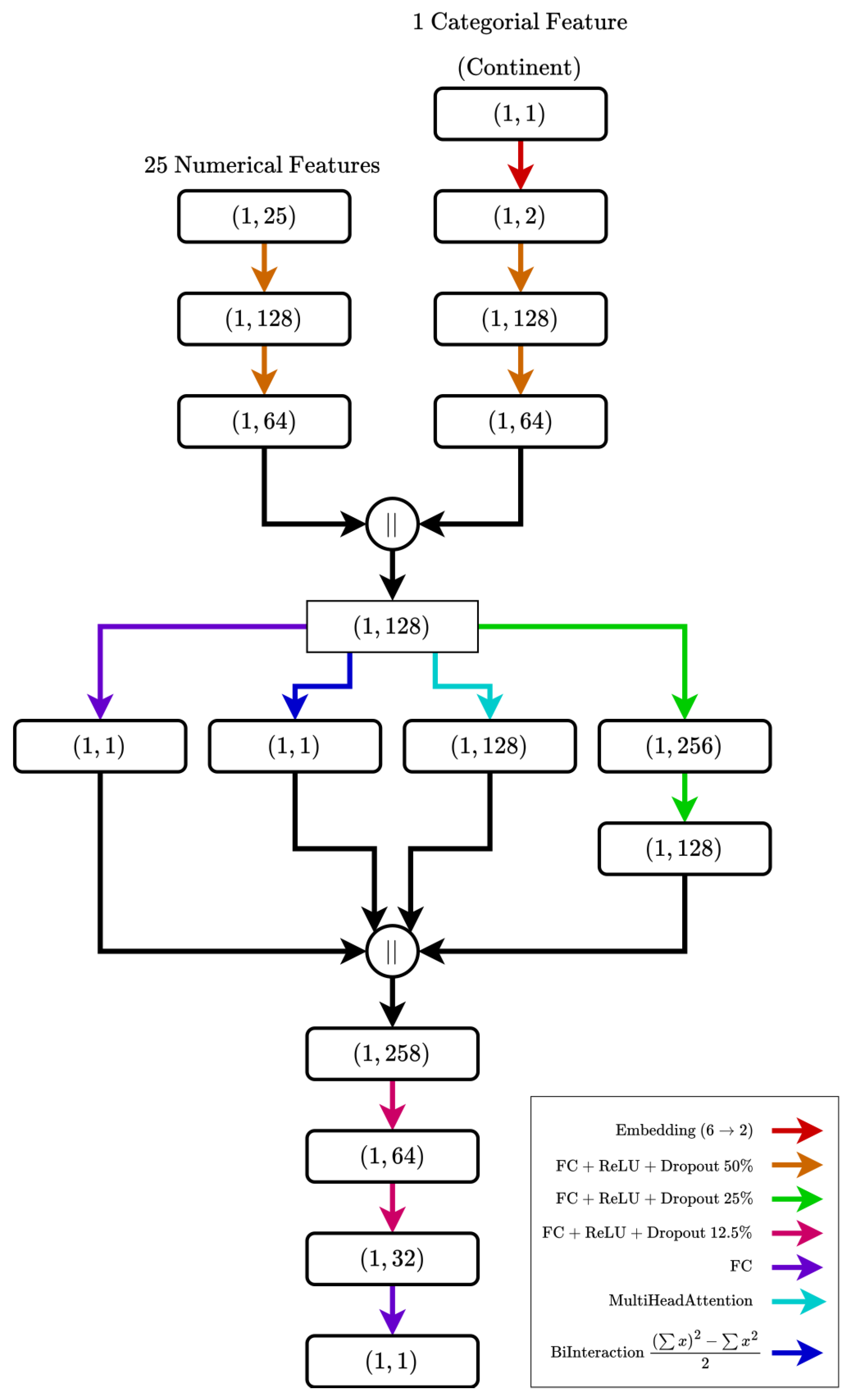
Figure 4 illustrates the regression architecture developed in this study, adapted from the NON framework to explicitly handle our structured input as a mix of numerical and categorical fields. The network begins by processing the 25 numerical features through a MLP composed of two fully connected layers with ReLU activations and 50% dropout, projecting each input from ( 1 , 25 ) ( 1 , 128 ) ( 1 , 64 ) . In parallel, the categorical ‘continent’ feature is embedded into a 2-dimensional vector ( 1 , 1 ) ( 1 , 2 ) and then passed through the same MLP structure. The resulting 64-dimensional outputs are concatenated into a unified 128-dimensional vector that captures field-level representations. This joint embedding is then enriched via four parallel transformation paths: a linear projection to a scalar, a bilinear interaction computing ( x ) 2 x 2 2 , a Multi-Head Attention layer producing a 128-dimensional output, and a deeper MLP stack ( 128 256 128 ) with ReLU, batch normalization, and 25% dropout. The outputs of these four components are concatenated into a 258-dimensional vector, which is passed through a final fusion MLP ( 258 64 32 1 ) with decreasing dropout (12.5%) and a final linear layer that outputs the predicted annual temperature increase. This design effectively combines local feature representations with higher-order global interactions, tailored to the complex dependencies observed in environmental data.
In terms of training configuration, the NON model was fine-tuned to minimize the MSE loss over a maximum of 50,000 epochs with mini-batches of 128 samples, using the Adam optimizer (learning rate 10 3 , weight decay 10 5 ). We employed early stopping-halting training if the validation R2 failed to improve for 2000 consecutive epochs, and a ReduceLROnPlateau policy to multiply the learning rate by 0.9 after 200 stagnant epochs. Dropout was applied after every dense layer, decaying from 50% in the initial layers to 12.5% in the final fusion block, which curbed early co-adaptation while preserving the network’s capacity for higher-order feature interactions. These settings produced the highest validation R2 of other tested configurations, demonstrating its higher suitability to capture both local and global patterns underlying annual temperature increase.

2.2.7. Multilayer Perceptron (MLP)

The Multilayer Perceptron (MLP) is a standard deep learning architecture that is able to capture complex nonlinear relationships in supervised learning tasks. Specifically, it defines a mapping function by composing multiple layers of linear transformations and nonlinear activations. Given an input vector x, the model produces the predicted output as follows
y ^ ( x ) = W ( L ) σ σ ( W ( 1 ) x + b ( 1 ) ) + b ( L )
where W ( ) and b ( ) represent the weights and biases of layer , and σ ( · ) denotes the activation function. Under this formulation, an MLP-based regression model can be trained by minimizing a loss function computed between the predicted output and the ground-truth values, using backpropagation and gradient descent.
In our setting, each input sample consisted of 25 numerical variables and the categorical ‘continent’ feature, which was one-hot encoded, i.e., represented as 6 binary indicator variables (one per continent), resulting in a total of 31 input dimensions. The MLP was configured with three hidden layers of widths 32, 128, and 32 respectively, each followed by a ReLU activation and a Dropout layer with a rate of 30%. As training objective, we adopted the MSE loss, promoting stable convergence and penalizing large deviations in temperature predictions. The network was trained for 50,000 epochs using mini-batches of size 128 and the Adam optimizer with a learning rate of 10 3 and 2 weight decay of 10 5 . Early stopping was also implemented after 1000 epochs without improvement in validation R2, and the learning rate was reduced by a factor of 0.8 if the metric plateaued for 200 epochs. This configuration offers a compromise between model capacity and regularization, allowing the MLP to learn complex interactions among features while reducing the risk of overfitting in our environmental prediction task.
Although the models evaluated in this benchmark offer complementary strengths, their limitations should also be acknowledged. Gradient-boosted tree methods such as XGBoost, while accurate and robust, require careful hyperparameter tuning and can be computationally demanding during model selection, which may increase training time and the risk of overfitting if regularization or early stopping are not properly applied. Neural network architectures, by contrast, tend to be less effective for structured tabular data and often require larger datasets and stronger regularization to achieve stable performance. Recognizing these trade-offs is important for understanding the scope and applicability of each model family.

2.3. Evaluation Metrics

To assess how accurately each model predicts temperature variations, we rely on the five complementary regression metrics presented in this section. In combination, they are able to capture different aspects of predictive performance, allowing an objective comparison of how well each algorithm translates CO2-emission patterns into reliable forecasts of annual temperature change. In what follows, we denote the size of the test set by n, and the true and predicted temperature increase for the i-th sample by y ( i ) and y ^ ( i ) , respectively.

2.3.1. Mean Squared Error

The Mean Squared Error (MSE) function quantifies the average squared deviation between predictions and observations [47]
MSE = 1 n i = 1 n y ( i ) y ^ ( i ) 2 .
Because the squaring term emphasizes large discrepancies, this metric is particularly useful when large errors are deemed unacceptable, especially in a climate change context. In this study, MSE is reported in ( C ) 2 .

2.3.2. Mean Absolute Error

The Mean Absolute Error (MAE) averages the absolute residuals [47]
MAE = 1 n i = 1 n | y ( i ) y ^ ( i ) | ,
providing an easily interpretable typical error in the units of the target variable. In our case, MAE is expressed in °C and offers an intuitive measure of the annual misestimation.

2.3.3. Coefficient of Determination

The coefficient of determination (R2) quantifies how well the predicted values reproduce the true data while penalizing systematic bias. It expresses the proportion of the total variance in annual temperature change that is correctly captured by the model [47]
R 2 = 1 i = 1 n y ( i ) y ^ ( i ) 2 i = 1 n y ( i ) y ¯ 2 ,
where y ¯ is the empirical mean of the true target values in the test set. A value of 1 indicates perfect fidelity. Values below 0 show that the model performs worse than the mean predictor. In this case, R2 is dimensionless.

2.3.4. Explained Variance

The Explained Variance (EV) quantifies the fraction of variability captured by the predictions without penalizing for potential systematic bias [48]
EV = 1 Var y ( i ) y ^ ( i ) Var y ( i ) .
Here, Var ( · ) represents the empirical variance computed across the test set. When considered together with R2 the metric helps to separate variance capture from consistent over- or underestimation. EV is also dimensionless.

2.4. Explainable Artificial Intelligence Methods

To better understand which input features most influence model predictions, we adopted the two explainability tools presented in this section: Impurity-based Feature Importance and Shapley Additive Explanations (SHAP). These methods help reveal how different variables contribute to predicted temperature changes, enabling the identification of key drivers behind model decisions. This interpretability is essential for translating technical results into actionable insights that inform climate policy and guide effective mitigation planning.

2.4.1. Impurity-Based Feature Importance

For ensemble models based on decision trees, such as random forests and gradient boosting machines, feature importance can be quantified by measuring the total reduction in squared-error impurity across all splits where a feature is used. Specifically, for each split in each tree, the decrease in impurity is recorded and subsequently averaged over the entire ensemble (mean decrease in impurity). In this way, a feature that contributes to significant impurity reductions across many splits can be considered more influential to the final prediction. This method is computationally efficient and aligns directly with the training objective. However, it tends to overestimate the importance of features with many distinct values and is logically limited to tree-based models. In our work, we used the normalized impurity reductions obtained from the trained tree-based models to construct a coarse global ranking of feature relevance.

2.4.2. Shapley Additive Explanations

To complement the analysis of feature contributions, the SHAP (SHapley Additive exPlanations) framework proposed by Lundberg et al. [29] was employed. SHAP is a game-theoretic approach to explain the output of any ML model, based on the computation of Shapley values from cooperative game theory. It attributes to each feature the change in the model output when including that feature, averaged over all possible feature orderings. Given a model f and an input x = ( x 1 , , x p ) , the SHAP values ϕ j for each feature j satisfy the following additive decomposition
f ( x ) = ϕ 0 + j = 1 p ϕ j
where ϕ 0 represents the expected value of the model prediction across the training data, and each ϕ j denotes the marginal contribution of feature j to the deviation from ϕ 0 . Formally, the SHAP value for a feature j is defined as
ϕ j = S { 1 , , p } { j } | S | ! ( p | S | 1 ) ! p ! f S { j } ( x S { j } ) f S ( x S )
where S denotes a subset of features not containing j, and f S ( x S ) is the model’s prediction when only the features in S are present. Intuitively, this expression measures how much the inclusion of each feature changes the model’s prediction, on average, across all possible combinations of features. Each ϕ j can therefore be interpreted as the individual contribution of feature j to the specific prediction f ( x ) , positive when it increases the output and negative when it decreases it. The principal advantage of SHAP is its model-agnostic nature, which allows a unified framework for explaining the predictions of ML algorithms, including tree ensembles, neural networks, and generalized additive models. Furthermore, it ensures properties of local accuracy, consistency, and missingness, resulting in feature attributions that are mathematically correct and reliable.
The graphical representation of SHAP values, namely the SHAP summary plot, arranges features by decreasing importance (mean absolute SHAP value) and shows for each feature the distribution of SHAP values across all samples. Positive SHAP values indicate that the feature increases the model output relative to the baseline, whereas negative values imply a decreasing effect. The color encoding typically reflects the original feature value, allowing the identification of monotonic or non-monotonic relationships between features and predictions.
In this work, SHAP values were computed for all the considered regression models, including tree-based ensembles and deep learning models. For tree-based models, the TreeSHAP algorithm was employed to calculate exact SHAP values in polynomial time. For non-tree models, KernelSHAP was utilized as a model-agnostic approximation. The global importance of each feature was estimated by averaging the absolute SHAP values across the test set. These values were visualized through SHAP summary plots, which combine feature importance with the direction and magnitude of each feature’s effect on model output. While SHAP values are inherently in the same units as the model output (°C), all visualizations used consistent axes to facilitate qualitative comparison across models.

3. Results and Discussion

This section provides a detailed examination of the experimental results, combining quantitative comparisons, model interpretability analyses, case-specific evaluations, and local error investigations. In Section 3.1, we first present a comparative assessment of all regression models using tabular metrics, scatter plots, and residual analyses, highlighting their predictive accuracy and generalizability. Next, Section 3.2 synthesizes model interpretability insights through SHAP values and feature importance rankings, identifying common patterns and divergences across methods. Section 3.3 focuses on a case study that compares Iran’s emission profile with global trends, uncovering unique national characteristics and their implications. Finally, Section 3.4 presents an error analysis based on SHAP force plots and outlier diagnostics, shedding light on individual prediction behaviors and revealing conditions under which the models succeed or fail. This helps identify edge cases and evaluate model reliability in high-impact settings.

3.1. Comparative Model Performance

Table 2 provides a comprehensive comparison of the seven machine learning models and the Linear Regression baseline evaluated in this study, based on four standard performance metrics computed on the held-out test set: MSE, MAE, R2, and EV. Lower values are better for error-based metrics (MSE, MAE), whereas higher values indicate better performance for variance-explaining metrics (R2, EV). These results allow us to jointly assess the accuracy, robustness, and generalization capability of each model.
To contextualize the rationale behind the selected models, we first establish a Linear Regression model as a simple baseline. As shown in Table 2, this baseline model performs poorly (MSE = 0.59, R2 = 0.40), failing to capture even half of the variance in the test data. This result indicates that, although spatio-temporal features such as Year and Lat/Lon are informative, their relationship with temperature is markedly non-linear. A single global linear function cannot approximate either the accelerating warming trend (Figure 2a) or the heterogeneous spatial patterns across regions (Figure 2b). Consequently, the weak performance of the linear baseline provides empirical support for employing models with non-linear capacity.
With this baseline established, the results reveal a clear performance hierarchy. Gradient-boosted tree ensembles occupy the top tier, with XGBoost achieving the lowest error across the board (MSE = 0.27, MAE = 0.38) and explaining 73% of the variance, marginally ahead of both Gradient Boosting and LightGBM (MSE ≈ 0.29, R2 ≈ 0.71). The improvement over a standard Random Forest (MSE = 0.33, R2 = 0.66) illustrates how the sequential error-correction in boosting leads to more accurate annual temperature rise forecasts than the independent aggregation used in simple bagging. A second tier is formed by GRANDE (MSE = 0.37, R2 = 0.63), whose jointly trained tree ensemble lags the boosting trio, but still outperforms neural baselines. The gap widens for NON (MSE = 0.46) and vanilla MLP (MSE = 0.49), both of which retain barely half of the target variance. These initial figures suggest that for medium-sized datasets in environmental modeling that combine numerical and categorical variables, large parametric networks struggle to generalize, whereas tree ensembles, especially when boosted, translate the heterogeneous feature space into accurate, low-bias estimates. Our results are consistent with earlier studies on agricultural emission modeling, where gradient-boosted trees also outperformed other regression methods [22,23]. This agreement reinforces the robustness of ensemble approaches, while the comparatively weaker performance of deep networks in our setting reflects the data size and tabular structure, as similarly noted by Harsanyi et al. [24].
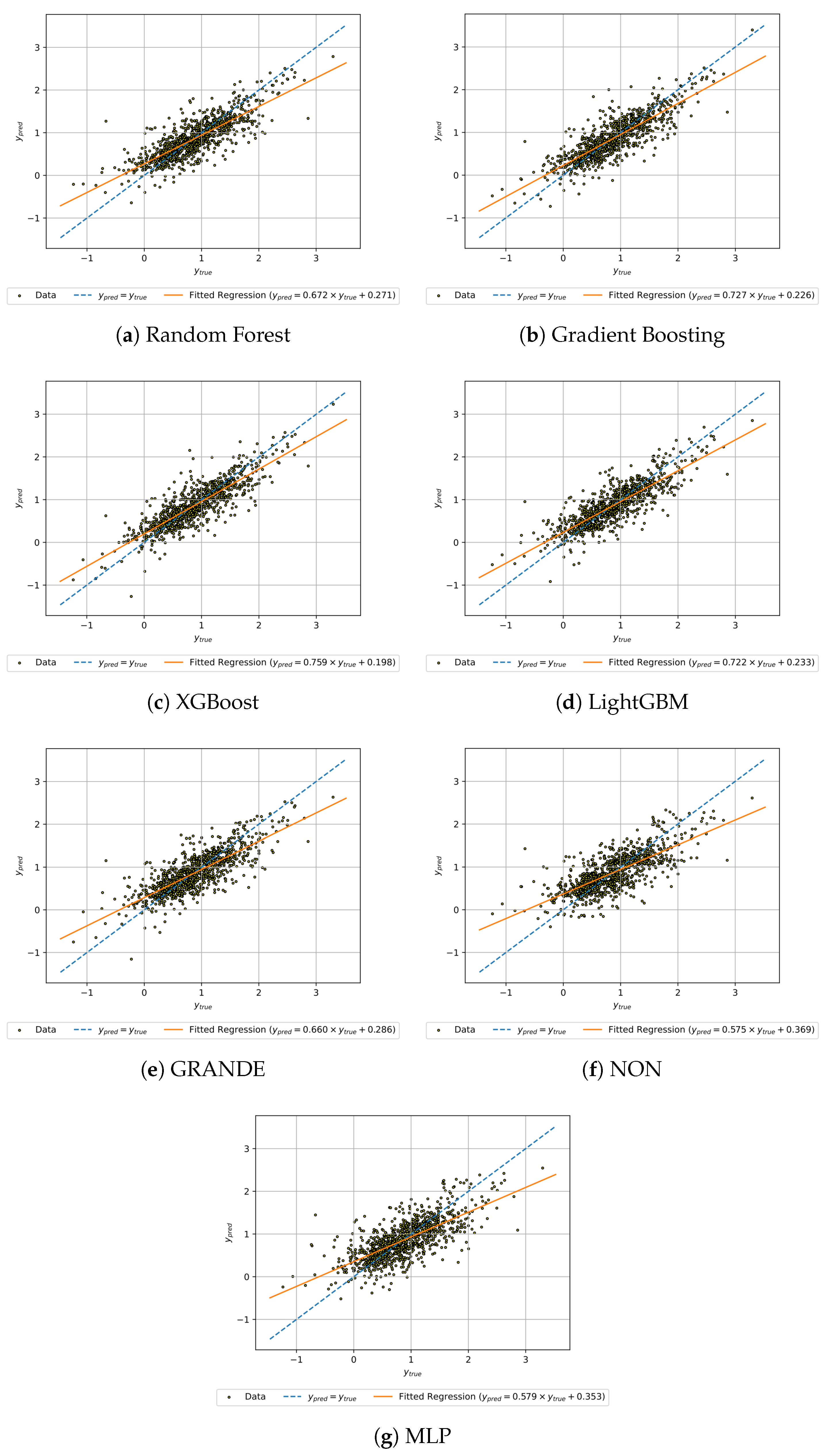
To translate these numerical rankings into a more intuitive understanding of each model’s strengths and weaknesses, we now turn to a detailed analysis of scatter plots and residual histograms. Figure 5 presents the scatter plots of predicted versus real values for each of the seven regression models evaluated in this study. Each subplot shows the ideal prediction line ( y pred = y true , dashed blue) alongside a fitted regression line (solid orange) to visualize systematic biases. These plots provide a graphical assessment of the predictive accuracy, error dispersion, and generalization behavior of each model. A tighter clustering of points around the diagonal indicates better agreement between predictions and ground truth, while systematic deviations highlight model-specific tendencies to under- or overestimate.
The diagrams in Figure 5 visually reinforce the performance hierarchy identified in the quantitative metrics. Boosted tree ensembles (XGBoost, Gradient Boosting, and LightGBM) show tight clustering around the identity line, with regression slopes near unity and minimal intercepts, indicating strong calibration and a faithful reproduction of the full dynamic range of annual temperature increases. These models are particularly effective at capturing extreme cases, both high- and low-emission scenarios, demonstrating their ability to generalize across diverse geopolitical and environmental contexts. In contrast, Random Forest approximates the overall trend but shows a shallower slope and increased vertical dispersion, suggesting a tendency to compress extreme predictions. This behavior, consistent with its higher MSE and lower R2, reflects the bias of the model toward the mean due to its independent tree averaging strategy. GRANDE shows a similar pattern, but with wider residual variance, reinforcing its intermediate performance between bagging and boosting approaches. Deep learning models such as NON and MLP visibly collapse their predictions to the mean of the data set, as indicated by regression slopes well below one and limited variance around the central cluster. This pattern is indicative of underfitting, consistent with the limited capacity of the models to capture nonlinear interactions and spatial dependencies embedded in agricultural emission data.
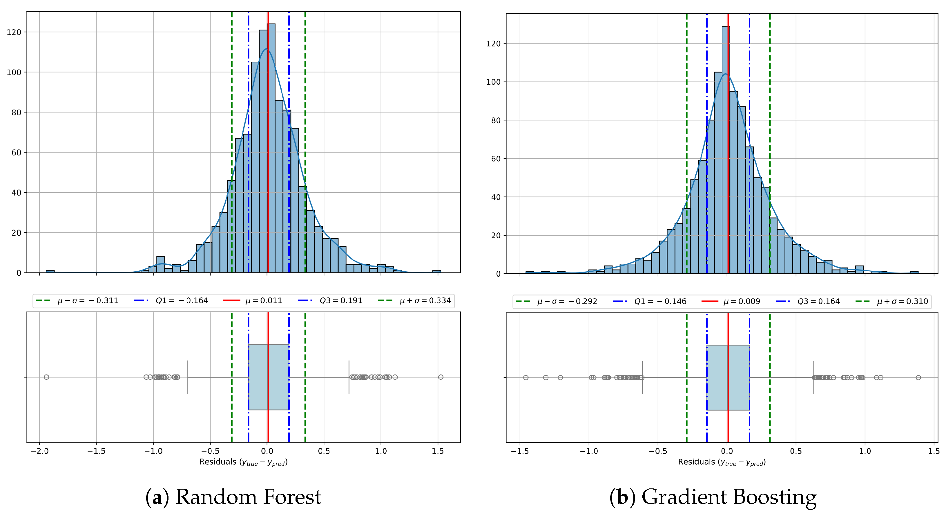
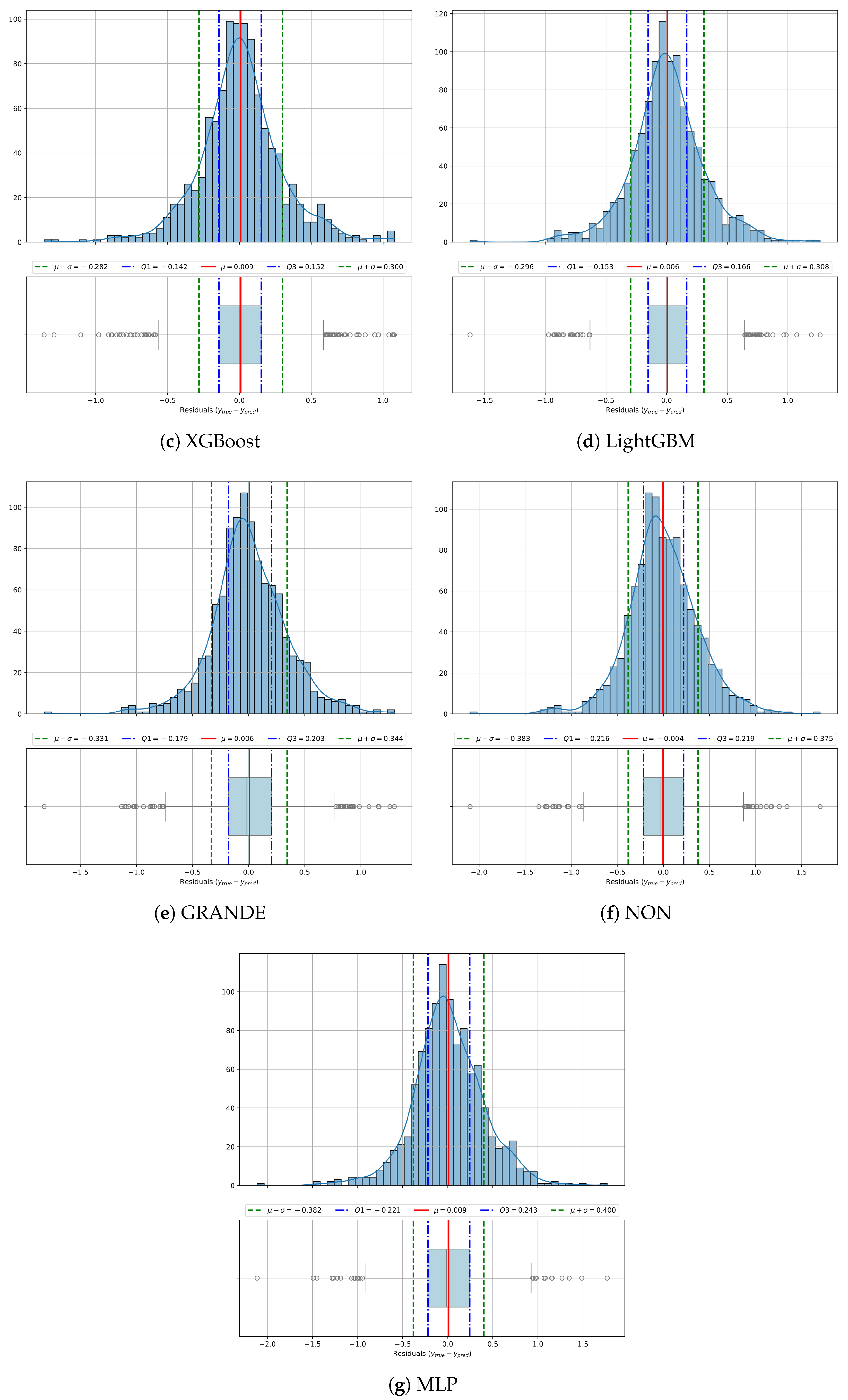
In order to complement the scatter plot analysis and gain deeper insight into the reliability and distribution of model errors, Figure 6 displays residual histograms and box plots for each regression method. These visualizations summarize how the prediction errors of each model are distributed around zero, providing clues about bias, variance, symmetry, and the presence of outliers. A narrow, centered, and symmetric histogram indicates consistent and unbiased performance, while wider or skewed distributions, as well as heavy tails, suggest instability, systematic bias, or sensitivity to certain samples. By comparing the shape, spread, and frequency of outliers across models, we can assess their robustness and error consistency under diverse conditions.
The residual distributions in Figure 6 provide a more granular perspective on prediction errors across models. Boosted methods once again emerge as the most effective, with XGBoost showing a mean residual close to zero ( μ = 0.009 ), low variability ( σ = 0.298 ), and a narrow interquartile range ( Q 1 = 0.150 , Q 3 = 0.148 ), which reflects stable and unbiased predictions with few extreme errors. Gradient Boosting and LightGBM perform similarly, maintaining symmetric error profiles centered near zero, although with slightly wider dispersion (approximately σ = 0.30 ). Random Forest ( σ = 0.323 ) and GRANDE ( σ = 0.328 ) display broader distributions, pointing to greater error variability and more frequent moderate misestimations. In contrast, NON and MLP exhibit flatter and wider residual curves with more pronounced tails. For example, NON reaches a standard deviation of 0.384, suggesting lower stability in the predictions. MLP also displays a slight negative skew, indicating a tendency to overestimate. These residual patterns support previous observations, confirming that boosted ensembles not only outperform in global metrics but also produce more consistent and reliable predictions on a case-by-case basis.
From an application point of view, these findings are particularly relevant for environmental forecasting and climate policy design. The ability of boosted ensemble methods to produce accurate, stable and well-calibrated predictions, even in the upper range of the temperature distribution, is crucial when modeling the impacts of agricultural CO2 emissions. If warming in high-emission countries is underestimated, the result could be overly optimistic mitigation targets and inadequate policy responses. In contrast, the strong generalization capacity and low prediction bias shown by XGBoost, Gradient Boosting, and LightGBM ensure that national emission variability is faithfully captured in the forecasts. This level of reliability makes these models especially appropriate for supporting scenario analysis, emission benchmarking, and early warning systems, particularly in regions with limited data availability. In sum, the predictive behavior of tree-based ensemble methods aligns well with the demands of climate-sensitive planning, establishing them as valuable tools for environmental impact assessment.

3.2. Model Interpretability

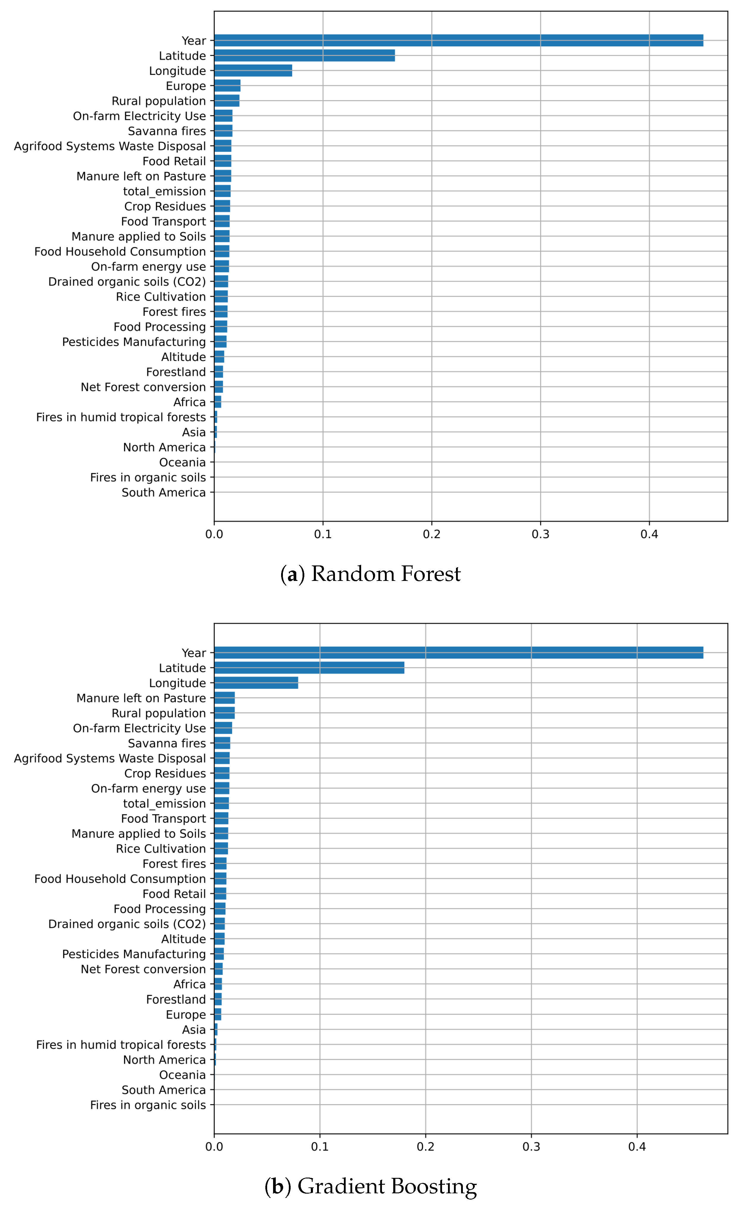
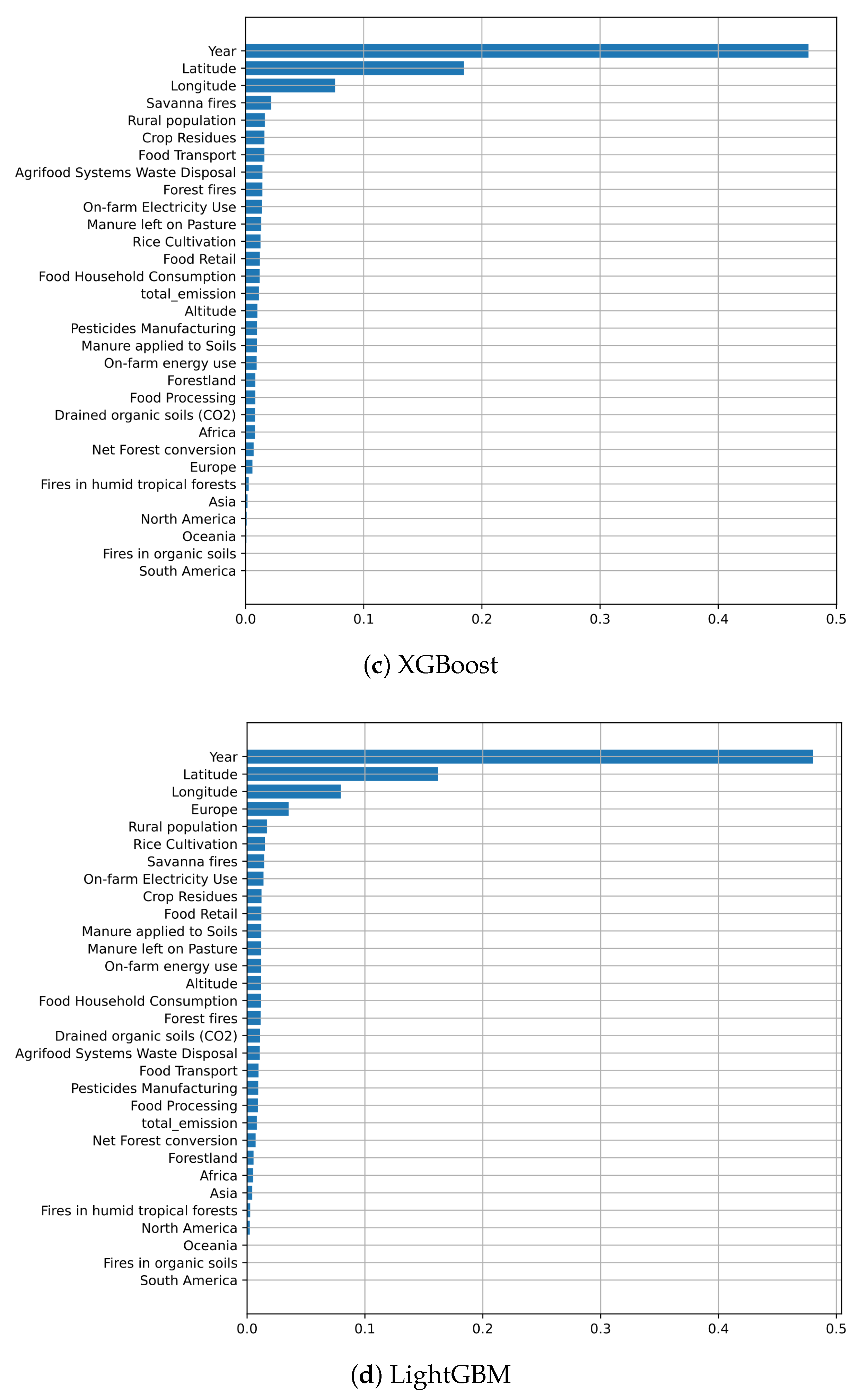
Here, we explore model interpretability through SHAP values and feature importance rankings. Rather than presenting findings model-by-model, this section synthesizes key insights into a comparative analysis that highlights both shared patterns and meaningful differences across algorithms. We begin with the feature importance scores obtained from the tree-based regressors. Figure 7 displays the normalized contribution of each input variable to the reduction of impurity during training. This visualization provides a broad perspective on which input categories, such as temporal, spatial, or environmental characteristics, play the most significant role in determining the model predictions. These rankings help to clarify how different types of information influence the learning process and guide the behavior of the ensemble methods.
The feature importance rankings in Figure 7 exhibit a striking consensus among the tree-based regressors. All models consistently assign the highest importance to temporal and spatial predictors, particularly ‘Year’, ‘Latitude’, and ‘Longitude’. These three characteristics dominate the impurity reduction process in all models, confirming that the general warming trend and geographic location are the main drivers of variation in the annual temperature increase associated with agricultural CO2 emissions. In contrast, most environmental and sector-specific features, such as ‘Savanna fires’, ‘Crop Residues’, and ‘Rice Cultivation’, occupy lower ranks, often contributing less than 5% to the model’s decisions. Some socio-economic features like ‘Rural population’ or ‘On-farm Electricity use’ register modest importance in select models, but generally remain secondary. This pattern suggests that, while granular environmental factors may shape local emission profiles, it is the broader spatio-temporal structure that most effectively informs predictive modeling in this domain. It is crucial to note that this dominance does not imply that simpler, linear models are sufficient. On the contrary, it reinforces the need for the advanced models benchmarked in this study. The high predictive performance is achieved precisely because these ML models, unlike linear ones, can capture the critical, non-linear interactions between the dominant spatio-temporal drivers and the secondary, sector-specific features.
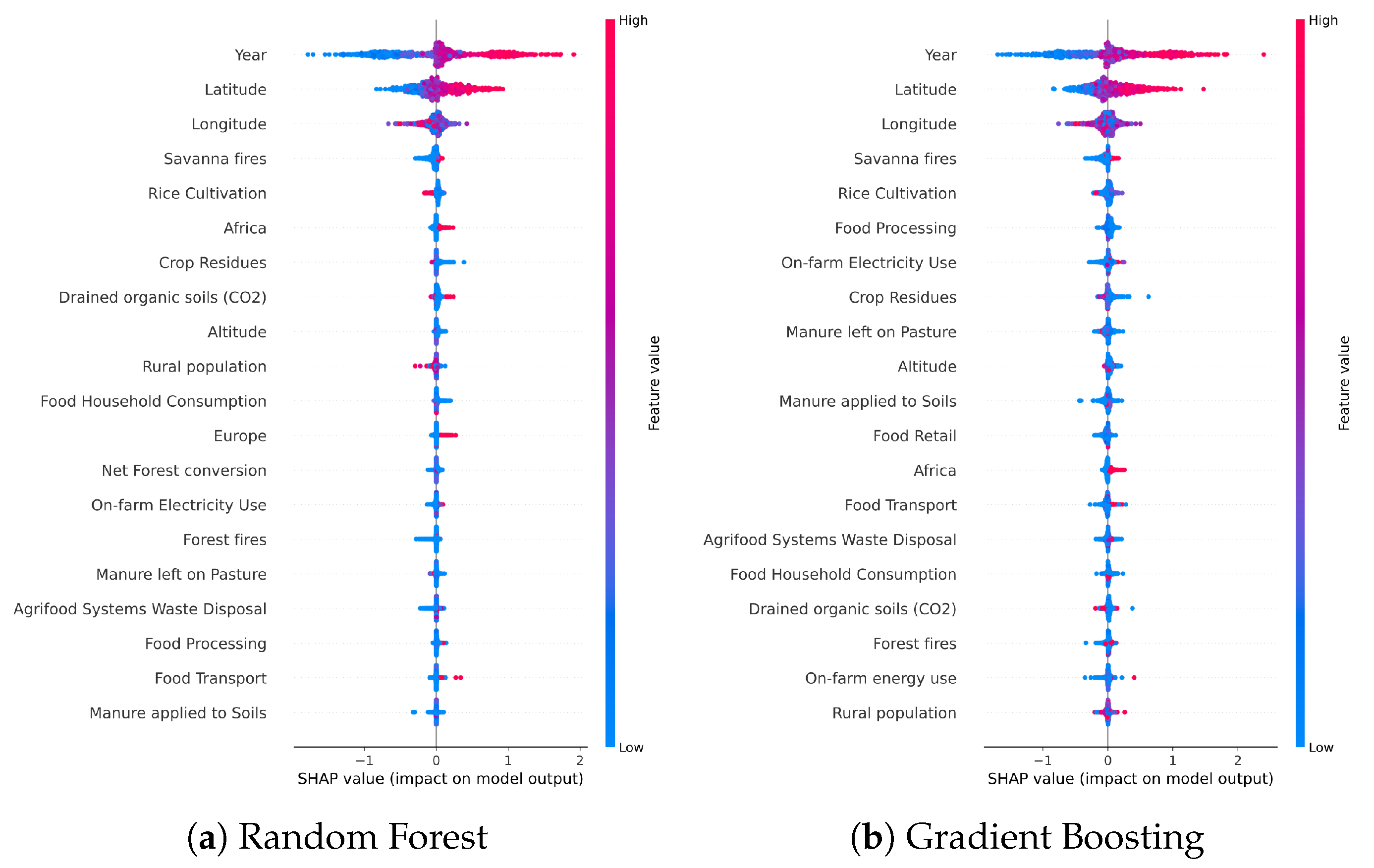
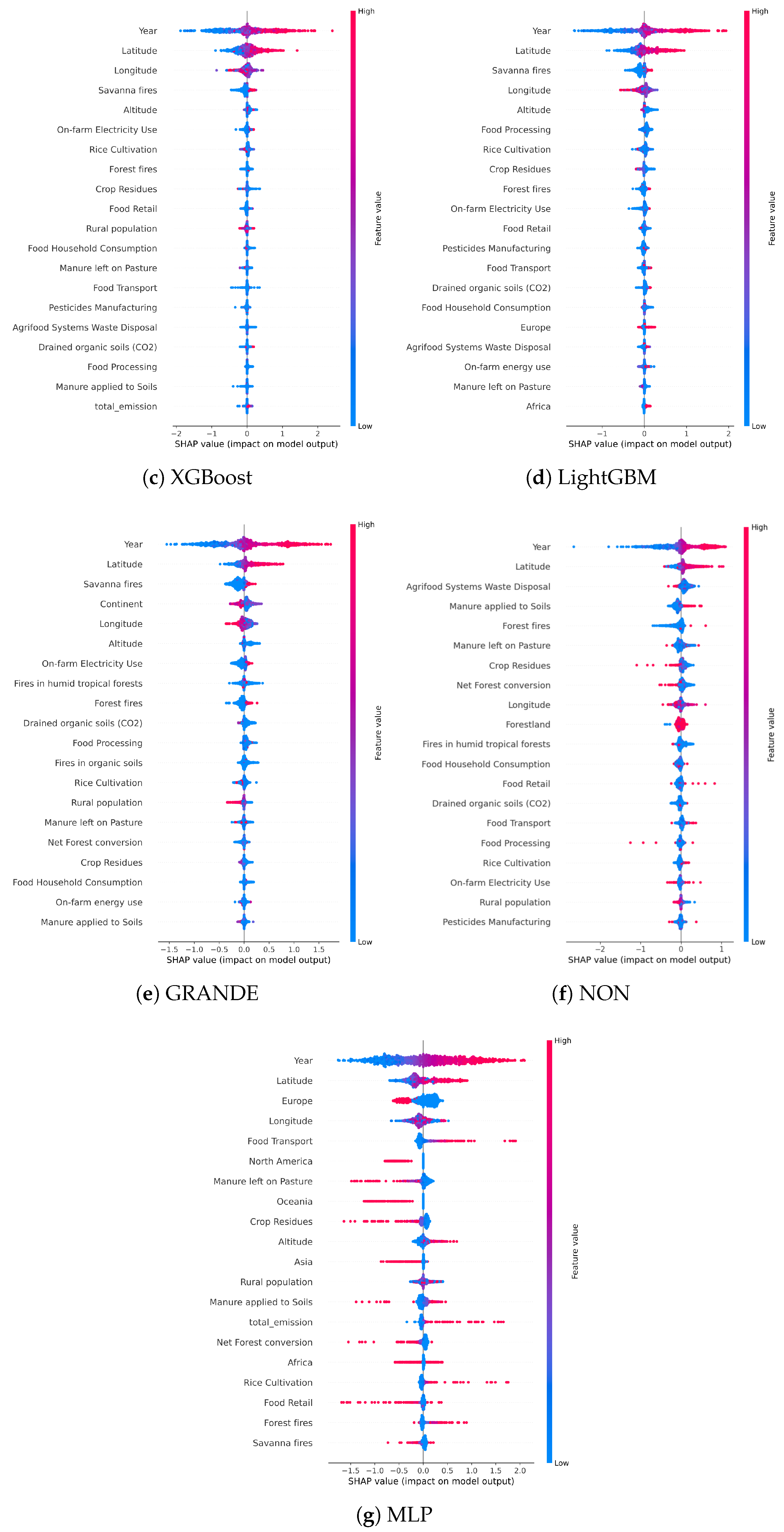
To broaden the interpretability analysis and include all model types, we next examine SHAP values. While traditional feature importance metrics are only applicable to tree-based models, SHAP offers a unified, model-agnostic framework that attributes each prediction to specific input features. This is particularly useful for understanding the behavior of neural networks such as NON and MLP, where native importance rankings are not available. Figure 8 presents SHAP summary plots for each regressor, highlighting both the magnitude and direction of feature contributions. These visualizations help identify not only which variables matter most, but also how they interact with predictions across different value ranges.
The SHAP diagrams in Figure 8 provide a detailed and comparative view of feature contributions across models, revealing not only consistent trends but also subtle differences in how each algorithm processes the input data. As previously observed, ‘Year’, ‘Latitude’, and ‘Longitude’ consistently emerge as the most influential variables, reaffirming the dominant role of spatiotemporal context in shaping predictions of agricultural CO2-induced warming. However, the SHAP distributions offer further nuance. In models such as XGBoost and NON, the broad range of SHAP values associated with ‘Year’ suggests that temporal dynamics exert varying degrees of influence depending on architecture. ‘Longitude’ frequently displays high variance, symmetric spreads (particularly in LGBM and Random Forest), hinting at complex regional interactions or latent feature entanglement. Environmental features including ‘Savanna fires’, ‘Rice Cultivation’, and ‘On-farm Electricity use’ exhibit stronger and more directional impact in GRANDE, NON, and MLP, indicating their importance in models with higher capacity for local or nonlinear structure. In contrast, tree-based models consistently downplay these variables, perhaps due to the dominance of stronger global signals. Socio-demographic and categorical features such as ‘Europe’, ‘North America’, and ‘Oceania’ show wide SHAP dispersions in neural networks, supporting the idea that these architectures integrate regional encodings to capture latent economic and institutional variation. Additionally, variables like ‘Food Transport’ and ‘Manure left on Pasture’ contribute meaningfully to MLP, and ‘Agrifood Systems Waste Disposal’ and ‘Manure applied to Soils’ show strong positive impact in NON, reflecting broader agri-environmental system effects. The feature ‘Rural population’ exhibits high directional variance, sometimes boosting predictions, sometimes damping them, underscoring its entangled role across models. Similarly, ‘Altitude’ appears with a consistent, though weak, negative contribution in several regressors, likely reflecting indirect effects related to land use or elevation patterns. Finally, while intuitively relevant, variables such as ‘Forest fires’ or ‘Crop Residues’ remain marginal across models, suggesting redundancy or multicollinearity with more dominant inputs. Together, these insights reaffirm that boosted trees excel at isolating strong global predictive signals, while deep networks can capture more context-specific or interaction-driven relationships, offering complementary perspectives on the drivers of warming.
All these interpretability findings reinforce the practical value of combining high-performance models with transparent diagnostics. For stakeholders involved in climate-sensitive planning (such as agricultural ministries, environmental agencies, or international policy bodies), the ability to trace predictions back to specific regional, environmental, or temporal factors is crucial. The prominence of spatio-temporal features across models confirms the importance of location and trajectory in emission forecasting, while the selective sensitivity of neural networks to localized or sector-specific variables suggests their utility in exploratory analysis or targeted intervention design. Importantly, SHAP results help identify not only the dominant predictors but also those whose impact varies significantly between models or contexts, such as ‘Rural population‘ or ‘Savanna fires’. These signals can guide data collection priorities, improve scenario testing, and enhance trust in model outputs by making their behavior more intelligible to non-technical decision-makers. Ultimately, interpretability is not merely a diagnostic tool, it is a bridge between technical modeling and actionable climate strategy.

3.3. Case Analysis: Iran vs. Global

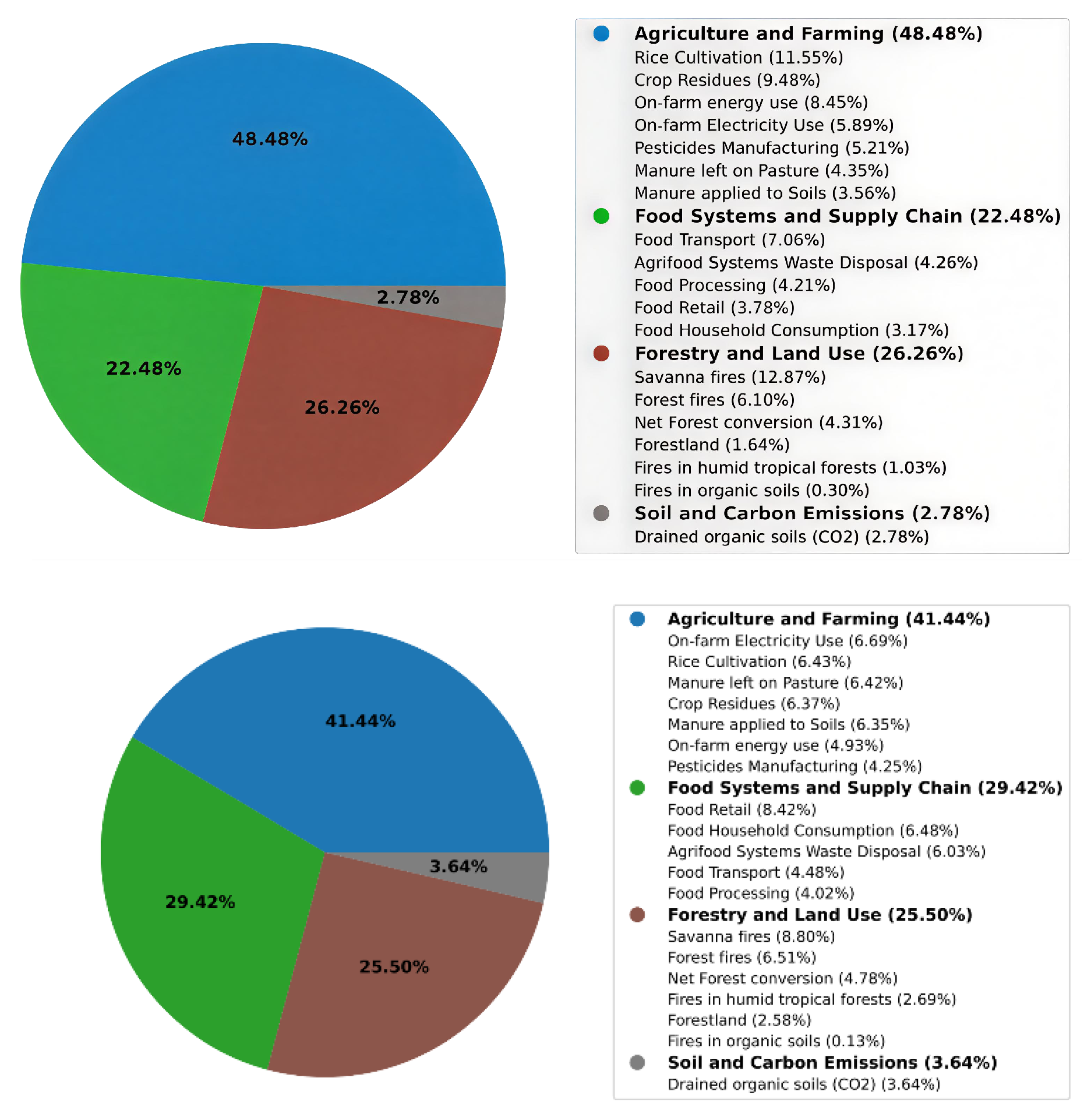
While the previous sections focused on global modeling and interpretability trends, this subsection provides a focused case study of Iran. Given its status as a top greenhouse gas emitter and its unique agroenvironmental profile, Iran offers a compelling opportunity to assess how national characteristics diverge from global patterns. To that end, we analyze the distribution of feature importance derived from mean normalized SHAP values in the XGBoost model, contrasting Iran-specific samples against global trends. These contrasts are visually summarized in Figure 9, which displays the relative contribution of grouped environmental characteristics to temperature predictions for Iran (top) and the global dataset (bottom).
The analysis highlights marked contrasts in the forces that shape temperature change at national and global scales. In the Iranian case, agriculture is clearly the dominant factor: the variables linked to this sector explain 48.48% of the model’s output, well above the 41.44% observed worldwide. Much of this gap is due to the weight of ‘Rice Cultivation’, which alone contributes 11.55%—almost double the influence of the next agricultural variable, ‘Crop Residues’. The figure mirrors Iran’s dependence on flooded paddy systems, known for their methane release, and on other water-intensive crops. Energy inputs compound the picture: both ‘On-farm energy use’ and ‘On-farm Electricity Use’ carry greater importance in Iran than in the global set, signaling persistent inefficiencies in farm power systems.
The supply chain shows an inverse pattern. The features grouped under food processing, distribution, and consumption account for just 22.48% in Iran versus 29.42% worldwide. Although ‘Food Transport’ remains the main element in this group for Iran (7.06%), variables such as ‘Food Retail’ (3.78%) and ‘Household Consumption’ (3.17%) make only a modest appearance. This aligns with the relatively centralized and less consumer-driven food networks of the country, where shorter supply chains can reduce the relative weight of downstream activities.
Land use dynamics show a similar aggregate weight in both contexts: 26. 26% for Iran and 25. 50% globally, but the underlying composition differs significantly. In Iran, the attribution of models is dominated by ‘Savanna Fires’ (12.87%), a striking figure given the limited extent of the true ecosystems of the savannas in the country. This may reflect rangeland burning practices or inconsistencies in spatial classification. In contrast, the global profile distributes importance more broadly across ‘Tropical Forest Fires’ and ‘Net Forest Conversion’, reflecting well-documented deforestation dynamics in tropical regions.
Soil-related emissions play a minor role in both settings, although the category is 31% less prominent in Iran (2.78%) than globally (3.64%). This reduction is mainly due to the minimal relevance of ‘Drained Organic Soils’, which are uncommon in Iran’s arid landscapes. Other soil-associated variables, such as ‘Manure left on Pasture’ and ‘Manure applied to Soils’, also show lower importance in Iran, suggesting different fertilization practices or land use configurations relative to global norms.
A closer look confirms that Iranian emissions are more concentrated in a limited number of dominant sources. In particular, ‘Rice Cultivation’ and ‘On-farm energy use’ together account for over 40% of the agriculture-related attribution, while the global distribution is more diffuse across a broader set of contributing variables, each with lower individual weights. Similarly, the reduced contribution of ‘Food Retail’ and ‘Household Consumption’ reflects shorter supply chains and limited cold chain infrastructure—features that, if modernized, could increase emissions unless accompanied by robust efforts to decarbonize.
In sum, Iran’s attribution profile reflects structural and agroecological particularities: the reliance on water-intensive cropping systems, centralized food logistics and energy-intensive farming practices differentiates it from global averages. Effective mitigation strategies should therefore prioritize irrigation efficiency, electrification and upgrading of farm equipment, and decentralization of food distribution networks. At the same time, convergence with international priorities, such as sustainable land management, improved manure handling, and improved supply chain efficiency, is essential to achieve integrated climate goals.

3.4. Error Analysis

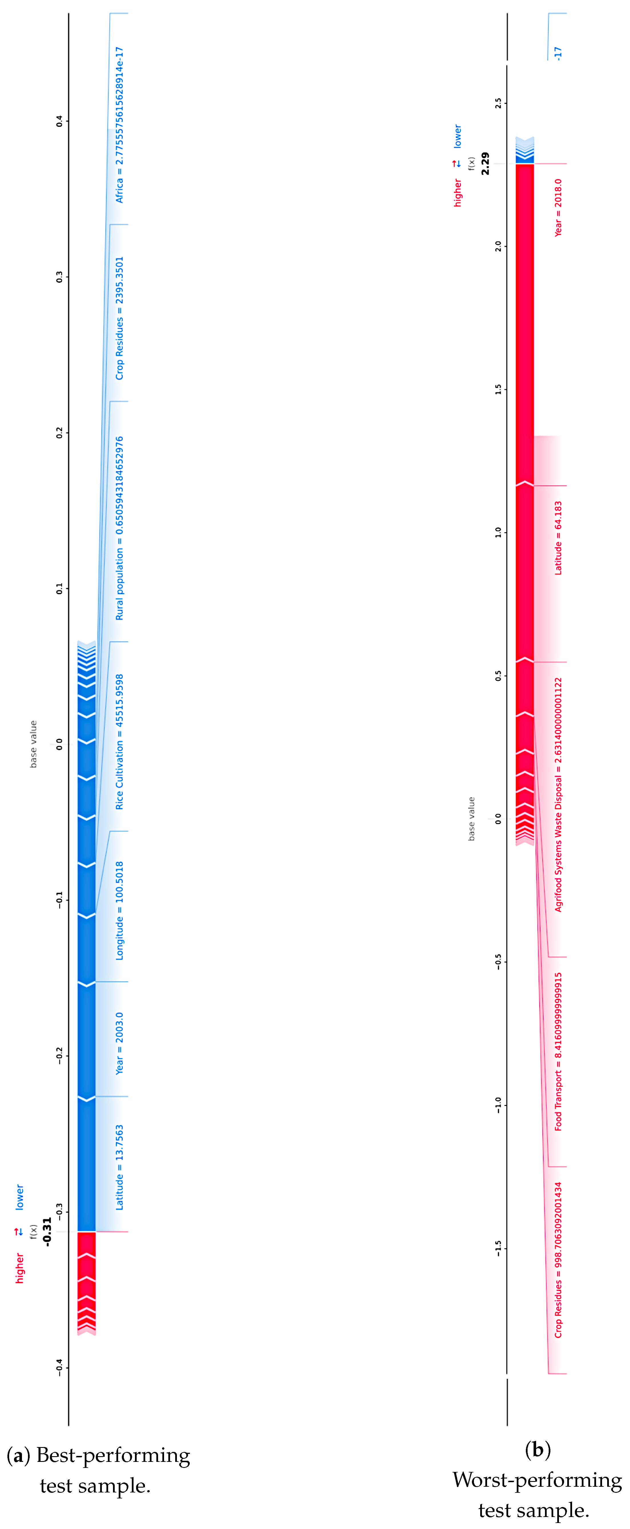
Beyond average performance metrics, understanding how and why models succeed or fail at the individual level is essential to build trust in predictive systems, particularly in high-stakes environmental modeling. Local interpretability techniques, such as SHAP force plots, allow for granular inspection of the model behavior in specific instances, highlighting the internal reasoning behind each prediction. This subsection leverages force plots to explore the extremes of model performance using XGBoost, the top-performing method in our evaluation. Figure 10 displays two representative samples: the most accurately predicted test instance (top panel) and the one with the highest prediction error (bottom panel), offering complementary insights into the model’s strengths and limitations.
In the best-predicted sample, the contribution of individual characteristics is relatively balanced, with no single variable disproportionately influencing the output. Key features such as ‘Year’, ‘Latitude’, and ‘Rice Cultivation’ exhibit moderate contributions that constructively align to approximate the true value, suggesting that the model correctly internalized the dominant patterns governing the sample’s emission-temperature relationship. This reinforces the validity of our core hypothesis that certain spatial-temporal and agro-environmental variables act as consistent predictors of warming trends and that tree-based ensemble methods are capable of capturing such interactions with high fidelity under typical conditions.
In contrast, the worst-performing prediction reveals signs of local overfitting or misalignment of the feature interaction. Notably, ‘Crop Residues’ and ‘Agrifood Systems Waste Disposal’ display strong positive SHAP values, collectively pushing the prediction well above the true temperature increase. This behavior suggests that in atypical samples, perhaps from countries with unique reporting patterns or extreme feature values, XGBoost may overestimate the impact of certain variables due to spurious correlations or limited contextual nuance. Such cases underscore the importance of integrating domain-specific priors or hybrid modeling strategies in future work. They also validate the inclusion of post hoc interpretability tools in our methodological pipeline, not just to explain average trends, but to diagnose and mitigate outlier behavior that could undermine policy relevance or stakeholder confidence.

4. Conclusions

This study developed a data-driven framework to analyze and predict the impact of agricultural CO2 emissions on annual temperature increase in 236 countries over a 30-year period. Using a diverse suite of regression models, including tree-based ensembles and deep neural architectures, we evaluated the capacity of representative machine learning (ML) techniques to forecast global warming trends from structured agri-environmental data. In parallel, we applied explainability tools (feature importance and SHapley Additive exPlanations (SHAP) values) to understand the drivers behind model predictions, both globally and in a focused national case study (Iran).
Our results show that gradient-boosted tree ensembles, particularly XGBoost, consistently outperform alternative models across all error and variance explanation metrics. These methods achieve high accuracy while maintaining interpretability, which makes them suitable for environmental forecasting. In contrast, deep learning models show weaker performance, likely due to their higher data requirements and lower inductive bias for tabular inputs. SHAP-based interpretability confirms that spatio-temporal features—especially ‘Year’, ‘Latitude’, and ‘Longitude’—are dominant predictors, with environmental and socio-economic variables playing more context-specific roles. Furthermore, local error analysis using SHAP force plots reveals that outlier predictions are often driven by exaggerated influence from less frequent emission sources, highlighting the need for context-aware regularization.
A key contribution of the study lies in the integrative use of predictive modeling and post hoc interpretability to reveal actionable insights. For example, the Iran case study demonstrated a pronounced national dependence on rice cultivation and on-farm energy use, contrasting with global trends that attribute greater weight to downstream supply chain emissions. These insights provide a concrete basis for region-specific mitigation strategies and policy design, offering a bridge between ML and sustainable development goals.
As with any data-driven study, this work has certain limitations. The use of nationally aggregated data, while useful for capturing general trends and enabling global comparisons, may also overlook important local variations in emission behaviors. Similarly, although SHAP provides valuable interpretability, its outcomes can be affected by feature interdependencies and model-specific characteristics. Moreover, the relatively modest performance of neural models probably stems from a combination of factors, including limited data, model complexity, and reduced inductive bias for tabular inputs, rather than the inherent unsuitability of deep learning approaches. Future work should consider hybrid models that combine expert knowledge with data-driven learning, incorporate additional remote sensing or land-use datasets, and explore causal inference techniques to strengthen the interpretability and robustness of predictions. In addition, integrating a formal uncertainty quantification component, such as the propagation of measurement errors or the use of probabilistic and Bayesian approaches, would be a valuable extension of the framework, providing a more explicit assessment of prediction confidence. Finally, extending the analysis to project future emissions under various policy or climatic scenarios would offer substantial value for forward-looking environmental planning.
Author Contributions

Conceptualization, R.P., S.S., D.S., R.F.-B., G.G.-M. and M.H.R.; Methodology, R.P. and S.S.; Software, S.S. and D.S.; Investigation, R.P., S.S., D.S., R.F.-B., G.G.-M. and M.H.R.; Visualization, R.P. and D.S.; Supervision, R.P., S.S., R.F.-B. and M.H.R.; Writing—Original Draft Preparation, R.P., S.S., D.S. and M.H.R.; Writing—Review & Editing, R.F.-B. and G.G.-M.; Funding Acquisition, G.G.-M. All authors have read and agreed to the published version of the manuscript.

Funding

This research was funded by project 1403/D/9/27530 from the University of Mohaghegh Ardabili, and by the Region of Murcia (Spain) through the Regional Program for the Promotion of Scientific and Technical Research of Excellence (Action Plan 2022), managed by Fundación Séneca - Agencia de Ciencia y Tecnología de la Región de Murcia, grant number 22130/PI/22.

Data Availability Statement

All datasets used in this study are publicly available. The primary dataset (Agri-food CO2 emission dataset—Forecasting ML) is accessible on Kaggle [36]. Geographic covariates were obtained from open sources: country coordinates [37] and average country elevation [38]. No proprietary or restricted-access data were used. The code to reproduce preprocessing, model training, and figures is openly available at GitHub: https://github.com/dorrin-sot/co2_emission_regression (accessed on 25 September 2025). For questions, please contact the maintainers (s.sabzi@gau.ac.ir, dorrin.sotoudeh@sharif.edu).

Conflicts of Interest

The authors declare no conflict of interest. The funders had no role in the design of the study; in the collection, analyses, or interpretation of data; in the writing of the manuscript, or in the decision to publish the results.

References

  1. Forster, P.M.; Smith, C.; Walsh, T.; Lamb, W.F.; Lamboll, R.; Hall, B.; Hauser, M.; Ribes, A.; Rosen, D.; Gillett, N.P.; et al. Indicators of Global Climate Change 2023: Annual update of key indicators of the state of the climate system and human influence. Earth Syst. Sci. Data 2024, 16, 2625–2658. [Google Scholar] [CrossRef]
  2. Intergovernmental Panel on Climate Change. Sixth Assessment Report—Synthesis Report. 2022. Available online: https://www.ipcc.ch/report/ar6/syr/ (accessed on 25 September 2025).
  3. Ding, Y.; Mu, C.; Wu, T.; Hu, G.; Zou, D.; Wang, D.; Li, W.; Wu, X. Increasing cryospheric hazards in a warming climate. Earth-Sci. Rev. 2021, 213, 103500. [Google Scholar] [CrossRef]
  4. Nicholls, R.J.; Lincke, D.; Hinkel, J.; Brown, S.; Vafeidis, A.T.; Meyssignac, B.; Hanson, S.E.; Merkens, J.L.; Fang, J. A global analysis of subsidence, relative sea-level change and coastal flood exposure. Nat. Clim. Change 2021, 11, 338–342. [Google Scholar] [CrossRef]
  5. Zittis, G.; Almazroui, M.; Alpert, P.; Ciais, P.; Cramer, W.; Dahdal, Y.; Fnais, M.; Francis, D.; Hadjinicolaou, P.; Howari, F.; et al. Climate change and weather extremes in the Eastern Mediterranean and Middle East. Rev. Geophys. 2022, 60, e2021RG000762. [Google Scholar] [CrossRef]
  6. Solomon, S.; Daniel, J.S.; Sanford, T.J.; Murphy, D.M.; Plattner, G.K.; Knutti, R.; Friedlingstein, P. Persistence of climate changes due to a range of greenhouse gases. Proc. Natl. Acad. Sci. USA 2010, 107, 18354–18359. [Google Scholar] [CrossRef] [PubMed]
  7. Smith, S.J.; Chateau, J.; Dorheim, K.; Drouet, L.; Durand-Lasserve, O.; Fricko, O.; Fujimori, S.; Hanaoka, T.; Harmsen, M.; Hilaire, J.; et al. Impact of methane and black carbon mitigation on forcing and temperature: A multi-model scenario analysis. Clim. Change 2020, 163, 1427–1442. [Google Scholar] [CrossRef]
  8. Singh, A.; Pandey, A.K.; Santhosh, D.; Ganavi, N.; Sarma, A.; Deori, C.; Das, J.; Kumar, S. A comprehensive review on greenhouse gas emissions in agriculture and evolving agricultural practices for climate resilience. Int. J. Environ. Clim. Change 2024, 14, 455–464. [Google Scholar] [CrossRef]
  9. Li, L.; Awada, T.; Shi, Y.; Jin, V.L.; Kaiser, M. Global Greenhouse Gas Emissions From Agriculture: Pathways to Sustainable Reductions. Glob. Change Biol. 2025, 31, e70015. [Google Scholar] [CrossRef]
  10. Sauerbeck, D.R. CO2 emissions and C sequestration by agriculture–perspectives and limitations. Nutr. Cycl. Agroecosyst. 2001, 60, 253–266. [Google Scholar] [CrossRef]
  11. Santiago-De La Rosa, N.; González-Cardoso, G.; Figueroa-Lara, J.d.J.; Gutiérrez-Arzaluz, M.; Octaviano-Villasana, C.; Ramírez-Hernández, I.F.; Mugica-Álvarez, V. Emission factors of atmospheric and climatic pollutants from crop residues burning. J. Air Waste Manag. Assoc. 2018, 68, 849–865. [Google Scholar] [CrossRef]
  12. Laborde, D.; Mamun, A.; Martin, W.; Piñeiro, V.; Vos, R. Agricultural subsidies and global greenhouse gas emissions. Nat. Commun. 2021, 12, 2601. [Google Scholar] [CrossRef]
  13. Lokupitiya, E.; Paustian, K. Agricultural soil greenhouse gas emissions: A review of national inventory methods. J. Environ. Qual. 2006, 35, 1413–1427. [Google Scholar] [CrossRef]
  14. Butterbach-Bahl, K.; Kesik, M.; Miehle, P.; Papen, H.; Li, C. Quantifying the regional source strength of N-trace gases across agricultural and forest ecosystems with process based models. Plant Soil 2004, 260, 311–329. [Google Scholar] [CrossRef]
  15. Murad, W.; Islam Molla, R.; Bin Mokhtar, M.; Raquib, A. Climate change and agricultural growth: An examination of the link in Malaysia. Int. J. Clim. Change Strateg. Manag. 2010, 2, 403–417. [Google Scholar] [CrossRef]
  16. Hamrani, A.; Akbarzadeh, A.; Madramootoo, C.A. Machine learning for predicting greenhouse gas emissions from agricultural soils. Sci. Total Environ. 2020, 741, 140338. [Google Scholar] [CrossRef]
  17. Sharafi, S.; Kazemi, A.; Amiri, Z. Estimating energy consumption and GHG emissions in crop production: A machine learning approach. J. Clean. Prod. 2023, 408, 137242. [Google Scholar] [CrossRef]
  18. Safa, M.; Nejat, M.; Nuthall, P.; Greig, B. Predicting CO2 Emissions from Farm Inputs in Wheat Production using Artificial Neural Networks and Linear Regression Models. Int. J. Adv. Comput. Sci. Appl. 2016, 7, 268–274. [Google Scholar] [CrossRef]
  19. Sun, W.; Liu, M. Prediction and analysis of the three major industries and residential consumption CO2 emissions based on least squares support vector machine in China. J. Clean. Prod. 2016, 122, 144–153. [Google Scholar] [CrossRef]
  20. Pérez-Miñana, E.; Krause, P.J.; Thornton, J. Bayesian Networks for the management of greenhouse gas emissions in the British agricultural sector. Environ. Model. Softw. 2012, 36, 128–138. [Google Scholar] [CrossRef]
  21. Shiri, N.; Shiri, J.; Kazemi, M.H.; Xu, T. Estimation of CO2 flux components over northern hemisphere forest ecosystems by using random forest method through temporal and spatial data scanning procedures. Environ. Sci. Pollut. Res. 2022, 29, 16123–16137. [Google Scholar] [CrossRef] [PubMed]
  22. Adjuik, T.A.; Davis, S.C. Machine learning approach to simulate soil CO2 fluxes under cropping systems. Agronomy 2022, 12, 197. [Google Scholar] [CrossRef]
  23. Wu, Q.; Wang, J.; He, Y.; Liu, Y.; Jiang, Q. Quantitative assessment and mitigation strategies of greenhouse gas emissions from rice fields in China: A data-driven approach based on machine learning and statistical modeling. Comput. Electron. Agric. 2023, 210, 107929. [Google Scholar] [CrossRef]
  24. Harsányi, E.; Mirzaei, M.; Arshad, S.; Alsilibe, F.; Vad, A.; Nagy, A.; Ratonyi, T.; Gorji, M.; Al-Dalahme, M.; Mohammed, S. Assessment of Advanced Machine and Deep Learning Approaches for Predicting CO2 Emissions from Agricultural Lands: Insights Across Diverse Agroclimatic Zones. Earth Syst. Environ. 2024, 8, 1109–1125. [Google Scholar] [CrossRef]
  25. Xue, W. Deep learning algorithm-based carbon emission assessment of agricultural soils. In Proceedings of the 2023 8th International Conference on Intelligent Computing and Signal Processing (ICSP), Xi’an, China, 21–23 April 2023; pp. 1311–1314. [Google Scholar]
  26. Wang, H.; Mei, Y.; Ren, J.; Zhu, X.; Qian, Z. Multi-Scale Temporal Integration for Enhanced Greenhouse Gas Forecasting: Advancing Climate Sustainability. Sustainability 2025, 17, 3436. [Google Scholar] [CrossRef]
  27. Chen, Y.; Xie, Y.; Dang, X.; Huang, B.; Wu, C.; Jiao, D. Spatiotemporal prediction of carbon emissions using a hybrid deep learning model considering temporal and spatial correlations. Environ. Model. Softw. 2024, 172, 105937. [Google Scholar] [CrossRef]
  28. Luo, C.; Liu, Y.; Gao, P. Learning nonlinear feature interactions for tabular data. Proc. AAAI Conf. Artif. Intell. 2020, 34, 4811–4818. [Google Scholar]
  29. Lundberg, S.M.; Lee, S.I. A unified approach to interpreting model predictions. Adv. Neural Inf. Process. Syst. 2017, 30, 4768–4777. [Google Scholar]
  30. Grossman, G.M.; Krueger, A.B. Environmental Impacts of a North American Free Trade Agreement. 1991. Available online: https://www.nber.org/papers/w3914 (accessed on 25 September 2025).
  31. Han, T.T.T.; Lin, C.Y. Exploring long-run CO2 emission patterns and the environmental kuznets curve with machine learning methods. Innov. Green Dev. 2025, 4, 100195. [Google Scholar] [CrossRef]
  32. Guo, X.; Kou, R.; He, X. Towards Carbon Neutrality: Machine Learning Analysis of Vehicle Emissions in Canada. Sustainability 2024, 16, 10526. [Google Scholar] [CrossRef]
  33. Kreidenweis, U.; Lautenbach, S.; Koellner, T. Regional or global? The question of low-emission food sourcing addressed with spatial optimization modelling. Environ. Model. Softw. 2016, 83, 190–200. [Google Scholar] [CrossRef]
  34. D’Orazio, P.; Pham, A.D. Evaluating climate-related financial policies’ impact on decarbonization with machine learning methods. Sci. Rep. 2025, 15, 1694. [Google Scholar] [CrossRef] [PubMed]
  35. Shabani, E.; Hayati, B.; Pishbahar, E.; Ghorbani, M.A.; Ghahremanzadeh, M. A novel approach to predict CO2 emission in the agriculture sector of Iran based on Inclusive Multiple Model. J. Clean. Prod. 2021, 279, 123708. [Google Scholar] [CrossRef]
  36. Bello, A.L. Agri-Food CO2 Emission Dataset—Forecasting ML. 2022. Available online: https://www.kaggle.com/datasets/alessandrolobello/agri-food-co2-emission-dataset-forecasting-ml (accessed on 25 September 2025).
  37. Mooney, P. Latitude and Longitude for Every Country and State. 2020. Available online: https://www.kaggle.com/datasets/paultimothymooney/latitude-and-longitude-for-every-country-and-state (accessed on 25 September 2025).
  38. Wikipedia Contributors. List of Countries by Average Elevation. 2023. Available online: https://en.wikipedia.org/wiki/List_of_countries_by_average_elevation (accessed on 25 September 2025).
  39. Biau, G. Analysis of a random forests model. J. Mach. Learn. Res. 2012, 13, 1063–1095. [Google Scholar]
  40. Prasad, A.M.; Iverson, L.R.; Liaw, A. Comparing spatial regression to random forests for large environmental data sets. PLoS ONE 2020, 15, e0229509. [Google Scholar] [CrossRef]
  41. Friedman, J.H. Greedy function approximation: A gradient boosting machine. Ann. Stat. 2001, 29, 1189–1232. [Google Scholar] [CrossRef]
  42. Chen, T.; Guestrin, C. XGBoost: A Scalable Tree Boosting System. In Proceedings of the 22nd ACM SIGKDD International Conference on Knowledge Discovery and Data Mining, New York, NY, USA, 13–17 August 2016; pp. 785–794. [Google Scholar] [CrossRef]
  43. Ke, G.; Meng, Q.; Finley, T.; Wang, T.; Chen, W.; Ma, W.; Ye, Q.; Liu, T. LightGBM: A highly efficient gradient boosting decision tree. Adv. Neural Inf. Process. Syst. 2017, 30, 3149–3157. [Google Scholar]
  44. Bentéjac, C.; Csörgo, A.; Martínez-Muñoz, G. A comparative analysis of gradient boosting algorithms. Artif. Intell. Rev. 2021, 54, 1937–1967. [Google Scholar] [CrossRef]
  45. Marton, S.; Lüdtke, S.; Bartelt, C.; Stuckenschmidt, H. GRANDE: Gradient-based decision tree ensembles for tabular data. arXiv 2023, arXiv:2309.17130. [Google Scholar]
  46. Kingma, D.P.; Ba, J. Adam: A Method for Stochastic Optimization. In Proceedings of the International Conference on Learning Representations (ICLR), San Diego, CA, USA, 7–9 May 2015. [Google Scholar]
  47. Willmott, C. Some comments on the evaluation of model performance. Bull. Am. Meteorol. Soc. 1982, 63, 1309–1313. [Google Scholar] [CrossRef]
  48. McKay, M.; Donnelly, P.; Paradis, K.; Horgan, P.; Brennan, C.; Cole, J.; Worrell, F. Time to look at self-rated health: Do time attitudes scores explain variance in self-rated health beyond health indicators? Personal. Individ. Differ. 2024, 217, 112454. [Google Scholar] [CrossRef]
Figure 1. Class imbalance across continents in the full dataset.
Modelling 06 00153 g001
Figure 2. Exploratory analysis of the average temperature increase (°C) data (1990–2020), showing (a) the global trend, (b) continental trends, and (c) distributions by continent. These plots highlight the data’s non-stationarity, high volatility, and significant spatio-temporal heterogeneity.
Modelling 06 00153 g002
Figure 3. Flowchart illustrating the workflow adopted in this paper, highlighting model-specific preprocessing (encoding) and hyperparameter tuning approaches.
Modelling 06 00153 g003
Figure 4. A general overview of the developed NON architecture. Black arrows indicate the data flow, while colored arrows represent specific operations (e.g., Fully Connected layers, attention) as detailed in the embedded legend.
Modelling 06 00153 g004
Figure 5. Scatter plots of predicted vs. true values for each regression method. Dashed blue line: y pred = y true ; solid orange line: fitted regression.
Modelling 06 00153 g005
Figure 6. Residuals histograms (and box-plots) for each regression method. Dashed line marks the zero-error reference.
Modelling 06 00153 g006aModelling 06 00153 g006b
Figure 7. Normalized feature-importance rankings for each tree-based regression model. (a) Random Forest. (b) Gradient Boosting. (c) XGBoost. (d) LightGBM.
Modelling 06 00153 g007aModelling 06 00153 g007b
Figure 8. SHAP summary plots for each regression method, illustrating the contribution of each feature to the model’s output.
Modelling 06 00153 g008aModelling 06 00153 g008b
Figure 9. Grouped feature contributions to temperature predictions in Iran (top) and globally (bottom) based on SHAP values from the XGBoost model.
Modelling 06 00153 g009
Figure 10. SHAP force plots (rotated 90 degrees) for the best-performing (a) and the worst-performing (b) test samples using XGBoost. Bars represent the contribution of each feature to the deviation from the base value. Red features increase the predicted value, blue features decrease it.
Modelling 06 00153 g010
Table 1. Features of the Agri-food CO2 emissions dataset. All emissions are expressed in kilotonnes (kt) of CO2, except for ‘Rice Cultivation’ (CH4 emissions) and ‘total_emission’ (CO2-equivalent).
FeatureDescription
‘Area’Reporting country
‘Year’Calendar year
‘Savanna Fires’Emissions from fires in savanna ecosystems
‘Forest Fires’Emissions from fires in forested areas
‘Crop Residues’Emissions from burning or decomposition of crop residues
‘Rice Cultivation’Methane emissions from rice cultivation
‘Drained Organic Soils’Emissions from draining organic soils
‘Pesticides Manufacturing’Emissions from pesticide production
‘Food Transport’Emissions from food transportation
‘Forestland’Net CO2 sequestration by existing forests
‘Net Forest Conversion’Net emissions from land-use change (deforestation/afforestation)
‘Food Household Consumption’Emissions from household food consumption
‘Food Retail’Emissions from retail food sales
‘On-farm Electricity Use’Emissions from electricity use on farms
‘Food Packaging’Emissions from food packaging lifecycle
‘Agrifood Systems Waste Disposal’Emissions from waste disposal in agrifood systems
‘Food Processing’Emissions from industrial food processing
‘Fertilizers Manufacturing’Emissions from fertilizer production
‘IPPU’Emissions from industrial processes and product use
‘Manure Applied to Soils’Emissions from applying manure to agricultural soils
‘Manure Left on Pasture’Emissions from manure on grazing land
‘Manure Management’Emissions from manure treatment and storage
‘Fires in Organic Soils’Emissions from fires in organic soils
‘Fires in Humid Tropical Forests’Emissions from fires in humid tropical forests
‘On-farm Energy Use’Emissions from energy consumption on farms
‘Rural Population’Number of people living in rural areas
‘Urban Population’Number of people living in urban areas
‘Total Population—Male’Total number of male individuals
‘Total Population—Female’Total number of female individuals
‘total_emission’Total greenhouse gas emissions from all sources
‘Average Temperature’Average annual temperature change (°C)
Table 2. Performance comparison of regression models on the test set. Lower values indicate better performance for MSE and MAE, whereas higher values (closer to 1.0) are better for R 2 and EV. Best results are highlighted in bold.
ModelMSE (↓)MAE (↓)R2 (↑)EV (↑)
Linear Regression0.590.570.400.40
Random Forest0.330.420.660.66
Gradient Boosting0.290.390.710.71
XGBoost0.270.380.730.73
LightGBM0.290.400.710.71
GRANDE0.370.450.630.63
NON0.460.510.540.54
MLP0.490.520.510.51
Disclaimer/Publisher’s Note: The statements, opinions and data contained in all publications are solely those of the individual author(s) and contributor(s) and not of MDPI and/or the editor(s). MDPI and/or the editor(s) disclaim responsibility for any injury to people or property resulting from any ideas, methods, instructions or products referred to in the content.