Abstract
Accurate identification of plastic polymers is essential for effective recycling, quality control, and environmental monitoring. This study assesses how spectral derivative preprocessing affects the classification of six common plastic polymers: Polyethylene Terephthalate (PET), Polyvinyl Chloride (PVC), Polypropylene (PP), Polystyrene (PS), and both High- and Low-Density Polyethylene (HDPE and LDPE), based on Fourier Transform Infrared (FTIR) spectroscopy data acquired at a resolution of 8 . Using Savitzky–Golay derivatives (orders 0, 1, and 2), five machine learning algorithms, namely Multilayer Perceptron (MLP), Extremely Randomized Trees (ET), Linear Discriminant Analysis (LDA), Support Vector Classifier (SVC), and Random Forest (RF), were tested within a strict framework involving stratified repeated cross-validation and a final hold-out test set to evaluate generalization. The first spectral derivative notably improved the model performance, especially for MLP and SVC, and increased the stability of the ET, LDA, and RF classifiers. The combination of the first derivative with the ET model provided the best results, achieving a mean F1-score of 0.99995 (±0.00033) in cross-validation and perfect classification (1.0 in Accuracy, F1-score, Cohen’s Kappa, and Matthews Correlation Coefficient) on the independent test set. LDA also performed very well, underscoring the near-linear separability of spectral data after derivative transformation. These results demonstrate the value of derivative-based preprocessing and confirm a robust method for creating high-precision, interpretable, and transferable machine learning models for automated plastic polymer identification.
1. Introduction
The global surge in plastic production, rising from 234 million tons in 2000 to 460 million tons in 2019, has intensified plastic pollution, making it a critical environmental challenge. Moreover, only 9% of waste is recycled, while 22% is dumped in uncontrolled landfills or released into the environment [1].
A concerning consequence of plastic pollution is the spread of microplastics, which are synthetic particles smaller than 5 , highly resistant to degradation and persistent in various ecosystems, where they accumulate and enter the food chain [2,3]. Their presence is usually linked to the widespread use of industrial polymers such as Polyethylene Terephthalate (PET), Polyvinyl Chloride (PVC), Polypropylene (PP), Polystyrene (PS), and both High- and Low-Density Polyethylene (HDPE and LDPE), with applications in packaging, construction, and consumer products. These materials are valued for their durability, flexibility, and resistance, but also cause adverse effects on aquatic organisms and key ecological processes [3].
Microplastics come from primary sources like cosmetic microbeads and secondary sources created when larger plastics undergo physical fragmentation, chemical degradation, and biological processes in the environment. Their small size allows them to disperse through water, wind, and living organisms [2].
The identification and quantification of microplastics require precise techniques such as Fourier Transform Infrared (FTIR) and Raman spectroscopy, which are useful for chemically characterizing polymers. However, these methods have limitations, including low sensitivity for particles smaller than 5 and potential interference from fluorescence in Raman spectroscopy. Additionally, manual analysis is laborious, slow, and prone to subjective errors when managing large sample volumes or complex mixtures [4]. These limitations justify the need to develop automated and efficient tools for spectral data analysis. In this sense, Machine Learning (ML) offers a promising set of techniques to address this challenge by enabling the identification of complex patterns in large datasets. Furthermore, preprocessing spectral data can greatly improve the performance of ML models by accentuating subtle features and minimizing the effects of noise or unwanted baseline distortions in the spectra.
The use of machine learning on spectroscopic data for identifying and classifying materials, including plastics and microplastics, has been a focus of active research. Numerous studies have explored different combinations of preprocessing techniques and ML algorithms to enhance the accuracy and efficiency of these analyses. Table 1 presents a direct, synthesized comparison between manual interpretation and automated classification paradigms. The criteria selected (including analysis time, scalability, reproducibility, required expertise, sensitivity to noise, and adaptability to new materials) reflect key practical considerations for researchers, laboratory managers, and regulatory agencies evaluating these methodologies. This table is designed to serve as a quick-reference tool that highlights the inherent trade-offs and complementary strengths of each approach.

Table 1.
Comparative overview of manual versus machine learning–based spectral interpretation.
In spectroscopy, data preprocessing is essential for improving spectral quality and analytical precision; the literature emphasizes normalization methods like Min–Max scaling, Max-Abs normalization, sum of squares transformation, and Z-score standardization [10], as well as scatter compensation methods comprising standard normal variate (SNV), multiplicative scatter correction (MSC), and spectral derivatives processing, which help reduce variability unrelated to the chemical composition and improve the performance of the multivariate models [11].
Several studies have emphasized the importance of applying suitable preprocessing techniques to FTIR spectral data to enhance model performance and data quality. Besides normalization, baseline corrections are used to eliminate the spectral background, while smoothing filters, such as the Savitzky–Golay filter, help reduce noise and calculate derivatives by fitting a polynomial curve locally within a sliding window. This improves the spectral resolution and accuracy of multivariate models, especially in FTIR spectra, and its usefulness in deep preprocessing to address distortions from light scattering has also been recognized [12]. In practical studies, such as the one by Delwiche and Reeves [13], it has been shown that using first and second-order derivatives computed with the Savitzky–Golay filter enhances spectral resolution and increases accuracy in multivariate regression models. This is supported by a range of applications; for instance, Zheng et al. [14] evaluated various preprocessing methods (including first and second derivatives, MSC, SNV, and the Savitzky–Golay filter) to improve both the spectral quality and model accuracy.
Similarly, Sitorus et al. [15] detailed the application of normalization, MSC, SNV, first and second derivatives, and their combinations prior to building prediction models for adulteration detection. In the context of wood forensics, Garg et al. [16] applied a first-order derivative to ATR-FTIR spectra to highlight subtle chemical differences between wood species that are otherwise visually indistinguishable due to shared components such as cellulose, hemicellulose, and lignin. Additionally, Liu et al. [17] applied multiple preprocessing methods (derivatives, two-dimensional transformations, MSC, SNV, Savitzky–Golay, and their combinations) before building traditional chemometric models, which can effectively learn directly from raw spectra.
In this study, the primary preprocessing step involved computing the first derivative using the Savitzky–Golay filter, which calculates the derivative and performs polynomial smoothing to enhance spectral resolution and reduce unwanted effects such as baseline drift and background noise.
In terms of classification, various machine learning algorithms have been successfully applied to classify the FTIR spectra of plastics, including Convolutional Neural Networks (CNNs), Logistic Regression (LR), Multilayer Perceptrons (MLP), Support Vector Machines (SVMs), k-Nearest Neighbors (k-NNs), Gradient Boost (GB), Decision Trees (DTs), Naive Bayes (NB), and Random Forests (RFs). Their effectiveness varies based on the dataset’s dimensionality and characteristics [5,17,18]. For example, Liu et al. [17] reported an accuracy of 97.44% with a 1D CNN, Tian et al. [18] found that a CNN with a Savitzky–Golay filter outperformed DT and SVM in agricultural soils, and Enyoh and Wang [5] emphasized the strong performance of RF and MLP in classifying aged PET.
Following this sequence of ideas, the primary objective of this research is to evaluate and compare the performance of a preprocessing technique based on spectral derivatives, combined with different ML algorithms for accurately classifying the six most common types of industrial plastics (PET, HDPE, PVC, LDPE, PP, and PS) from their FTIR spectra. The purpose is to demonstrate that this combination can offer a straightforward, effective, and reliable solution for automating microplastic identification, thereby enhancing environmental monitoring methods.
Our approach distinguishes itself and complements existing work in several ways. First, we use a public dataset of FTIR spectra from six common industrial polymers (PET, HDPE, PVC, LDPE, PP, and PS), with 500 samples for each [19], which facilitates reproducibility and comparison with future studies. This dataset spans a wide wavenumber range from 4000 to 400 , covering important regions of the mid-infrared that contain characteristic information about the polymers’ molecular bonds. Second, our main preprocessing focus is the systematic application of the first and second spectral derivatives, calculated with the Savitzky–Golay filter. Although derivatives are not entirely new in spectroscopy, exhaustively evaluating them across multiple ML algorithms for this specific dataset and examining their effect on class separation is a contribution of this work. We explore how derivatives help reduce baseline and noise issues inherent in spectral data. Third, we evaluate a specific set of classification algorithms: Multilayer Perceptron (MLP), Linear Discriminant Analysis (LDA), Extremely Randomized Trees (ETs), Random Forest (RF), and Support Vector Classification (SVC). The selection of these algorithms allows for comparing linear and non-linear models, as well as ensemble-based methods, providing a comprehensive view of their performance with preprocessed data. This set of algorithms may vary or constitute a particular combination that has not been extensively explored in previous works for this specific dataset and preprocessing technique.
Therefore, this study aims to advance the field by thoroughly evaluating the effects of preprocessing with derivatives across a broad spectral range and comparing the performance of various machine learning classifiers in identifying common plastics.
2. Materials and Methods
This section outlines the theoretical underpinnings, data resources, preprocessing steps, and machine learning techniques employed in this study, presenting the key concepts that sustain the methods and analysis of the results.
2.1. Machine Learning Techniques
Machine Learning (ML), a subset of Artificial Intelligence (AI), develops algorithms that autonomously enhance their task performance through data-driven learning, eliminating the need for case-specific programming [20]. In the context of this work, supervised learning is used, where the algorithm learns from a training dataset containing input examples (FTIR or Raman spectra) along with their corresponding output labels (type of plastic) [6,21]. This work aims to train a classifier with a strong generalization performance for novel inputs. The main approach is classification, which assigns a category (type of plastic) to each spectral sample. The process of learning from the training data is known as training, which is also referred to as fitting. Once the model is trained, it is evaluated on unseen data (test data) in a phase called testing, also known as predicting. These terms are often used interchangeably, but they reflect the two fundamental stages in supervised learning: learning patterns from known data and making predictions on new data.
For classifying plastic FTIR spectra, we chose a diverse set of machine learning algorithms representing different methodological approaches. We used a Multilayer Perceptron (MLP), a feedforward neural network capable of capturing complex, nonlinear decision boundaries. This approach has previously achieved average accuracies of 70.25% in similar FTIR-based polymer classification tasks [22,23].
In parallel, we included Linear Discriminant Analysis (LDA), a classical statistical method that projects data into a subspace to maximize inter-class separability, assuming Gaussian-distributed classes with shared covariance matrices [24]. While LDA provides interpretability and efficiency, its sensitivity to noise and limited performance on small or non-Gaussian datasets have led to the development of more robust extensions, which we explicitly considered in our experimental design.
To leverage the power of ensemble learning, we incorporated two tree-based methods: Random Forest (RF) and Extremely Randomized Tree (ET). RF operates through bagging, building multiple decision trees on bootstrapped samples and random feature subsets to reduce overfitting and improve generalization [25]; recent adaptations even include intuitionistic fuzzy logic to further enhance predictive accuracy [26]. ET expands this framework by introducing extra randomness in the choice of splitting thresholds, thereby lowering variance at a slight increase in bias. This trade-off is often helpful in high-dimensional spectral data [27].
Finally, we implemented Support Vector Classification (SVC), which finds the optimal separating hyperplane by mapping data into higher-dimensional spaces using kernel functions, including linear, polynomial, and Radial Basis Function (RBF) kernels. The choice of kernel and its hyperparameters is crucial in managing nonlinear class boundaries, making careful tuning essential for optimal performance on spectroscopic datasets [28].
The application of ML to this problem is motivated by its established effectiveness in uncovering complex, non-linear relationships within high-dimensional feature spaces, such as those generated by FTIR spectroscopy. ML algorithms can learn to distinguish between plastic types based on subtle differences in their spectral “fingerprints”, a task that is challenging to perform manually with high accuracy. This difficulty is particularly pronounced in post-consumer plastic waste (PCPW) spectra, where the presence of additives (e.g., organic pigments or calcium carbonate) and other contaminants can distort spectral bands and obscure identifying features [29]. The suite of algorithms detailed previously was therefore deliberately chosen to represent a range of diverse methodological approaches, including linear, neural network-based, and decision tree ensemble models, based on their reported success in similar classification tasks. It should be noted that the primary aim of this study was not an exhaustive hyperparameter tuning but rather a comparative assessment of how different preprocessing techniques affect classifier performance. Consequently, each model was implemented using its default hyperparameter settings.
2.2. Dataset
The dataset for this study was sourced from an open-access repository containing FTIR spectra of the six most common industrial polymers: Polyethylene Terephthalate (PET), Polyvinyl Chloride (PVC), Polypropylene (PP), Polystyrene (PS), High-Density Polyethylene (HDPE), and Low-Density Polyethylene (LDPE) [19]. The data were available at two resolutions, 4 (3736 features) and 8 (1869 features), where each feature represents a transmittance value. Although the higher resolution provides greater spectral detail, we selected the 8 dataset as a methodological choice to specifically evaluate the robustness and generalization capabilities of the ML models under less-than-ideal conditions, while also offering the ancillary benefit of minimizing computational demands. The transmittance values for each spectrum were generally within the 0–100 range, with occasional exceptions.
To facilitate their use with ML algorithms, the datasets were restructured. A column named ‘target’ was added to each dataset, containing the categorical label identifying the type of plastic for each sample (PET, HDPE, PVC, LDPE, PP, or PS). The remaining columns corresponded to spectral features (wavenumbers), and each row represents an individual sample with its respective transmittance values.
To provide a visual reference of the raw spectral data used in this study, Figure 1 displays randomly selected FTIR spectra (one per polymer class) drawn from the full dataset. These examples illustrate two common characteristics of the unprocessed spectra: the presence of high-frequency noise and a continuous, non-uniform background (baseline drift). While no quantitative analysis is derived from this figure, it serves a descriptive purpose: to contextualize the nature of the input data and to motivate the need for preprocessing, specifically baseline correction and noise reduction, prior to machine learning classification. This visual overview is intentionally placed here to help readers understand the starting conditions of the spectral data before any transformation is applied.
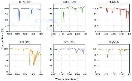
Figure 1.
Raw (unprocessed) FTIR spectra for each of the six polymer types, randomly selected from the dataset. The full spectral range (4000–400 cm−1) is displayed to illustrate common characteristics such as high-frequency noise and baseline drift, motivating the need for preprocessing. The corresponding sample number is indicated in parentheses.
2.3. Data Preprocessing: Spectral Derivatives
To formalize this preprocessing step, let the spectral intensity be defined as a function of the wavenumber , denoted by . In this formulation, represents the signal of interest, whereas denotes the baseline, which may assume constant, linear, or non-linear forms. In the specific case where the original spectrum includes a constant baseline B, the first derivative effectively eliminates it, as the derivative of a constant equals zero. Accordingly, the original spectrum (1) and its first derivative (2) can be expressed as follows:
In the case of a linear baseline, i.e., , the first derivative removes the constant term b, but retains an offset equal to the slope a. As illustrated in (3) and (4), the slope a remains as a constant offset in the differentiated signal.
For non-linear baselines, such as a quadratic function , the first derivative does not completely eliminate them but rather transforms them into lower-order terms. The result of applying the first derivative to the spectrum defined in (5) is given in (6):
For spectra with non-linear baselines, complete suppression of baseline distortions may require higher-order derivatives, such as the second derivative .
Spectral derivatives improve the ability to distinguish narrow peaks and subtle spectral features by reducing baseline effects, which is a key benefit when differentiating polymers with similar absorption profiles. However, direct numerical differentiation often amplifies high-frequency noise. To address this, we used the Savitzky–Golay filter, which calculates derivatives through local least-squares polynomial regression over a sliding window, providing smoothed derivative estimates that maintain peak shape and relative intensity [30].
In this context, using the original dataset (obtained at 8 resolution), we generated a single derived spectral set with first-order Savitzky–Golay derivatives. The filter parameters were selected empirically to balance noise suppression with the preservation of diagnostically important spectral features. The specific parameters for the Savitzky–Golay filter included a window length of 21 points and a second-order polynomial.
These values align with recommendations in specialized literature, such as Zimmermann and Kohler [31], emphasizing that proper tuning of window size and polynomial order significantly improves spectral resolution and signal-to-noise ratio in FTIR derivative analysis, while Sadeghi and Behnia [32] supports using second-order polynomials for spectral shape preservation and suggests minimizing the mean squared error (MSE) to select the optimal window.
2.4. Evaluation Metrics
The evaluation of the model performance was based on metrics derived from the confusion matrix, a fundamental tool for assessing classification models [33]. In this framework, a target class is designated as Positive (), with all other classes grouped as Negative (). As detailed in Table 2, the matrix compares the true class of an instance, y, against the class predicted by the model, .
Table 2.
Fundamental components of a confusion matrix for a class of interest.
A comprehensive suite of metrics was derived from the confusion matrix components: TP, TN, FP, and FN. The evaluation began with accuracy, calculated as the overall ratio of correct predictions (7). However, given that accuracy can be a misleading indicator on imbalanced datasets, a more nuanced set of metrics is often required [34].
Specifically, we assessed the trade-off between different types of errors using precision and recall. Precision, the ratio of true positives to all predicted positives (8), is critical when minimizing false positives is a priority [33]. In contrast, recall (sensitivity), the ratio of true positives to all actual positives (9), is paramount when the cost of false negatives is high [34]. The F1-score (10) was then used to provide a single performance measure that balances both Precision and Recall through their harmonic mean, which is especially valuable in the context of imbalanced classes [33,34].
Finally, to ensure a robust assessment that accounts for correct classifications occurring by chance, we employed two additional metrics. Cohen’s Kappa measures the level of agreement beyond random chance (11) [34]. The Matthews Correlation Coefficient (MCC) provides a correlation value between predictions and ground truth ranging from −1 to +1, where −1 indicates systematic disagreement (anti-correlation), 0 represents no correlation (random prediction), and +1 signifies perfect correlation (12). By utilizing all four values of the confusion matrix, MCC is considered a particularly reliable and unbiased metric for imbalanced datasets [34,35].
These metrics, used together, provide a strong and complete assessment of the classification models’ performance in the proposed task. For multiclass problems like in this study, metrics such as Recall and Precision, as well as F1, are usually calculated for each class and then averaged (for example, macro-average, where metrics are first calculated per-class then uniformly averaged, assigning equal importance to all classes).
2.5. Experimental Design and Modelling Methodology
The objective of this study was to rigorously evaluate how spectral derivative preprocessing affects the performance of machine learning classifiers on the FTIR spectra of six common polymers (PET, HDPE, PVC, LDPE, PP, and PS). Using data at a 8 resolution, the complete dataset of 3000 spectra (500 per polymer) was first randomly shuffled. A stratified split was then performed to create a training set (70%, 2100 samples) and a final hold-out test set (30%, 900 samples), ensuring proportional class representation. The test set was reserved exclusively for the final performance assessment to prevent data leakage. All stochastic operations were controlled with a fixed random seed of 42 for reproducibility.
To determine the optimal configuration, a comprehensive evaluation was conducted on the training set. This involved testing three spectral derivative orders (0, 1, and 2), calculated with a Savitzky–Golay filter (21-point window, 2nd-order polynomial), against five classifiers (MLP, LDA, ET, RF, and SVC). Each combination was assessed using a repeated stratified 5-fold cross-validation (10 repetitions), a method designed to provide reliable estimates of generalization performance and variability [36]. The configuration yielding the highest mean F1 score across the CV trials was selected as the optimal pipeline.
Following the selection process, a final model was trained on the entire 2100-sample training set using the identified optimal configuration. This model was then subjected to a single, final evaluation against the hold-out test set to obtain an unbiased estimate of its performance on unseen data. The evaluation was based on a comprehensive set of metrics: Accuracy, Recall, Precision, F1, Kappa, and MCC. The entire workflow was implemented in Python (v3.10) [37], leveraging key scientific libraries such as Scikit-learn [38] for modeling, with algorithm hyperparameters kept at their default values, Pandas [39] for data manipulation, NumPy [40] for numerical operations, and SciPy [41] for complementary scientific functions.
3. Results
This section presents the findings of the experiment on classifying FTIR spectra of six common plastic polymers, using a rigorous methodological approach to evaluate the impact of preprocessing through spectral derivatives and the performance of five machine learning algorithms.
3.1. Preliminary Data Findings: Baseline and Noise
As previously described, unprocessed FTIR spectra contain high-frequency noise and baseline contributions that may be constant, linear, or non-linear. The first derivative attenuates these effects in predictable ways: it fully eliminates constant baselines (2), reduces linear ones to a constant offset (4), and transforms non-linear baselines into lower-order terms (6).
To illustrate this behavior in practice, Figure 2 displays the FTIR spectrum of a representative PET sample alongside its first and second Savitzky–Golay derivatives. The original spectrum (Figure 2a) exhibits a pronounced, non-uniform background; after first differentiation (Figure 2b), this baseline is effectively suppressed, and subtle vibrational features become more distinct. The second derivative (Figure 2c) further enhances fine spectral structure (though at the cost of increased noise) confirming that higher-order derivatives may be necessary in cases of persistent non-linear baselines. This visual example reinforces the mathematical principles outlined above and motivates our choice of first-derivative preprocessing as the optimal balance between baseline removal and feature preservation.
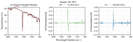
Figure 2.
FTIR spectrum of a PET sample. (a) The original spectrum (red line), its smoothed version (black line), and an estimation of the upper baseline (dotted black line). (b) The first derivative of the original spectrum, and (c) the second derivative. Note that in both cases the baseline disappears and spectral details are accentuated.
3.2. Results of Model and Derivative Selection by CV
CV on the training set allowed for a comparison of the performance of all combinations of classifier and derivative order. Table 3 summarizes the key metrics (Accuracy, Precision, Recall, F1, Kappa, and MCC) and fit times (Fit Time) for each combination.
Table 3.
Results of Repeated Cross-Validation (Mean ± Std. Dev.) on the training set (8 ). Fit Time (s) is the average fit time per fold. Best performance metrics (highest, or lowest for Fit Time) across all combinations are shown in bold.
The repeated and stratified cross-validation, performed on the training set, allowed for a detailed evaluation of the impact of different orders of spectral derivative (0, 1, and 2) on the performance of the five classifiers (MLP, LDA, ET, RF, and SVC). The complete results are presented in Table 3, while the main trends are discussed below, with a focus on the average F1 score and its standard deviation.
With the original spectrum (derivative 0), the MLP classifier showed a significantly lower performance (F1 = 0.44570 ± 0.22207), accompanied by ‘UndefinedMetricWarning’ warnings indicating difficulties in handling raw data without proper scaling transformation. In contrast, LDA (F1 = 0.99990 ± 0.00067), ET (F1 = 0.99905 ± 0.00151), RF, and SVC already demonstrated a very high performance with the original data.
In contrast, the impact of the spectra derivative was notable. The application of the first derivative resulted in a substantial improvement for MLP (F1 = 0.99957 ± 0.00103), which achieved a nearly perfect performance. It was with this first derivative that ET achieved the highest F1 among all combinations (0.99995 ± 0.00033), also exhibiting an extremely low standard deviation, suggesting high stability. LDA and RF also maintained or slightly improved their already excellent performance with the first derivative. SVC (F1 = 0.98843 ± 0.00442 with derivative 1) showed slightly lower performance compared to its performance with derivative 0, although it was still very high. With the second derivative, the results were, in general, very similar to those of the first derivative for MLP, LDA, ET, and RF, who continued with nearly perfect performance. However, SVC (F1 = 0.97329 ± 0.00722 with derivative 2) showed a noticeable decrease in performance and an increase in variability.
In a general comparison of classifiers, especially when considering the first derivative (which proved to be optimal overall), ET stood out not only for the highest F1, but also for its exceptional stability (lowest standard deviation). LDA was consistently one of the best-performing models, suggesting high linear separability of classes after derivative transformation. RF and MLP (the latter, once the derivative was applied) also proved highly competitive, with average F1s close to perfect. Although SVC obtained excellent F1s (above 0.988 with the first derivative), it was relatively the lowest performing and most variable among the top models in this configuration.
Regarding execution times (detailed in Table 3 and visualized in Figure 4), tree-based models (ET and RF) and LDA were, in general, the fastest to train. As expected, MLP and SVC tended to require longer fit times, an important consideration for applications with large volumes of data.
3.3. Visual Analysis of Cross-Validation
To better understand the behavior of different classifiers and derivative orders during the model selection phase, the cross-validation results were visually analyzed. Thus, Figure 3 presents the average F1 score obtained in cross-validation for each combination of classifier and spectral derivative order, along with their respective error bars indicating the standard deviation. The Y-axis has been segmented to clearly show both the full performance range and an expanded detail of the high-performance region (F1 > 0.965).
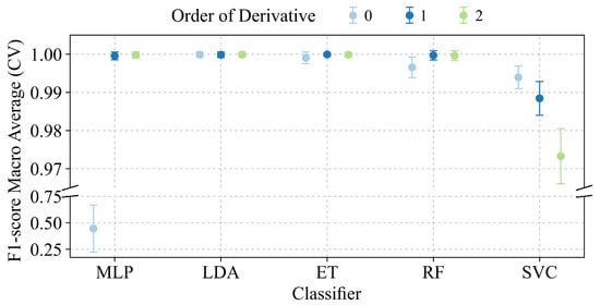
Figure 3.
Comparison of average F1 score (±Std. Dev.) obtained in CV for each combination of classifier and derivative order. The top panel shows a zoom into the high-performance region (F1 > 0.965), while the bottom panel shows the lower range to include MLP performance with derivative 0.
The visual analysis in Figure 3 complements the data in Table 3, allowing for the identification of performance trends and model stability. The results clearly show that the MLP classifier’s performance is highly dependent on derivative preprocessing. It performed poorly on the original spectrum (mean F1 ≈ 0.445) but achieved near-perfect scores (F1 > 0.995) with substantially lower variability after the application of first or second derivatives. Conversely, the LDA, ET, and RF classifiers consistently demonstrated an exceptional and stable performance (mean F1 ≈ 1.0) regardless of the derivative order. The SVC model, while also performing well, showed more sensitivity, achieving its best result (F1 > 0.99) on the raw spectrum and exhibiting a slight performance decay and increased variance with derived data.
Based on these observations, the ET model using the first derivative was selected as the optimal configuration. This combination achieves one of the highest mean F1 scores while also displaying one of the lowest standard deviations, a testament to its robustness and predictive reliability. Other strong candidates, such as LDA or RF with the first derivative, are also evident from the analysis.
In addition to these performance metrics, the computational efficiency of each combination was assessed by analyzing the average fit times from the CV, as shown in Figure 4.
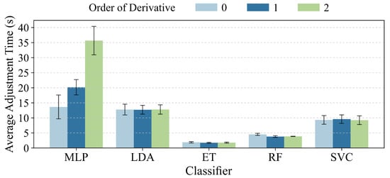
Figure 4.
Comparison of average fit time in seconds (±Std. Dev.) obtained in CV for each combination of classifier and derivative order.
As can be noted from Figure 4, ET and RF classifiers stand out as the fastest to train, with consistently low average fit times (generally below 5 s) for all three derivative orders. LDA also shows notable computational efficiency, with fit times slightly higher than tree-based models, but still very competitive (around 11–15 s). Applying derivatives does not seem to significantly impact the fit time of these three types of classifiers.
The MLP classifier presents considerably higher fit times in comparison. A trend is observed where the MLP fit time increases with the derivative order, being highest with the second derivative (approximately 31–40 s), followed by the first derivative (around 17–23 s), and derivative zero (around 10–17 s). This is expected, as neural networks typically require more computation for parameter optimization. Variability in fit times (error bars for one standard deviation) is also more pronounced for MLP, especially with derivatives 1 and 2.
Finally, the SVC classifier shows intermediate fit times, between LDA and tree-based models, but lower than MLP with derivatives 1 and 2. Times for SVC appear relatively consistent across different derivative orders (around 8–11 s), with moderate variability.
The information on fit times provided by Figure 4 is valuable for model selection in practical scenarios, where training efficiency can be a critical factor in addition to predictive accuracy. Considering the fit times along with performance metrics (shown in Figure 3), the trade-off between accuracy and efficiency can be evaluated. For example, ET with the first derivative was not only the model with the highest and most stable F1, but also one of the fastest to train. LDA, though slightly slower than ET, offers a near-perfect performance with very reasonable efficiency. While MLP achieves an excellent performance with derivatives 1 and 2, its higher computational cost could be a consideration in applications with large data volumes or time constraints.
3.4. Performance of the Final Model on the Test Set
For the selection of the optimal model and configuration, the average F1 score in cross-validation was used as the primary criterion, complemented by considerations of stability (low standard deviation) and computational efficiency. Based on these factors, the optimal configuration was identified as follows: (a) ET as the classifier, (b) application of the first derivative, and (c) an average CV F1 score of 0.99995 (±0.00033, Std. Dev.).
The optimal pipeline, consisting of preprocessing with the first spectral derivative and the ET classifier, was trained using the entire training set . Subsequently, its generalization ability was impartially evaluated on the final test set , which was not used in any prior model selection or tuning stage.
The quantitative results, presented in Table 4, show that the final model achieved a perfect performance (1.0) on all of the evaluated metrics (Accuracy, Recall, and Precision, F1, Kappa, and MCC) on this unseen dataset.
Table 4.
Evaluation metrics for the final model (ET, derivative 1) on the independent test set (8 ).
This perfect classification capability is clearly visualized in the normalized confusion matrix shown in Figure 5. The matrix presents a perfect diagonal, where 100% of the samples from each polymer class were correctly classified, without any instance of misclassification among the six categories (HDPE, LDPE, PET, PP, PS, and PVC). Each cell outside the main diagonal has a value of 0, indicating the total absence of false positives or false negatives.
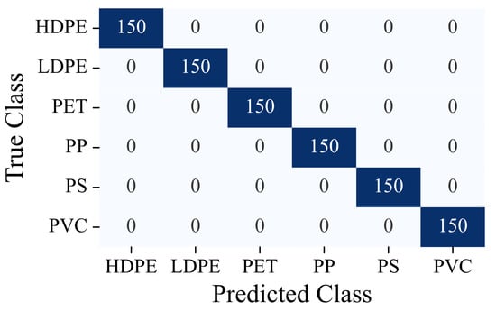
Figure 5.
Confusion matrix of the final model (ET, derivative 1) on the test set. A perfect diagonal with values of 150 indicates error-free classification for all polymer classes, while the lighter off-diagonal cells represent misclassifications, which are zero in this model.
This result confirms the model’s successful generalization from the training set to the test set, demonstrating that the chosen preprocessing-classifier combination enables perfect discrimination and separation among all six polymer classes within the FTIR spectral dataset. To validate these findings, we conducted three complementary analyses: (1) learning curves assessing model performance relative to training sample size, (2) validation curves evaluating parameter sensitivity, and (3) permutation tests verifying that the observed accuracy significantly exceeds chance-level classification. Together, these verification methods substantiate that the achieved separability stems from genuine spectral features rather than algorithmic artifacts or dataset peculiarities.
The learning behavior of the ET classifier under 5-fold cross-validation is illustrated in Figure 6. The X-axis represents the amount of training data (from ∼150 to 1680 samples), while the Y-axis shows the average macro F1-score. The training curve (blue) remains at 1.0 across all training sizes, while the validation curve (green) increases steadily until it converges with the training curve around 800–840 samples. From that point onward, both curves plateau at 1.0, and the confidence interval around the validation scores narrows significantly. This indicates that the model has reached a stable generalization performance.
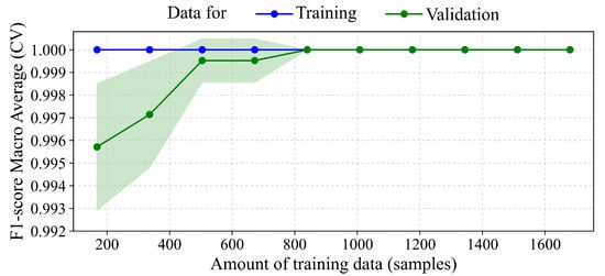
Figure 6.
Learning curve for ET classifier. The plot shows the average macro F1-scores across 5-fold cross-validation. The blue curve represents training performance, and the green curve shows validation performance, with the green shaded area representing ±1 Std. Dev. of the validation scores across the folds. From approximately 840 training samples (∼140 per class), the validation score converges with the training score, both reaching 1.0, indicating stable and optimal generalization performance.
Figure 7 shows the effect of varying the number of estimators (n_estimators) on the performance of the ET classifier, where each estimator corresponds to a randomly constructed decision tree. The training F1-score (blue) remains constant at 1.0 across all values. In contrast, the validation F1-score (green) rises sharply from 1 to 4 estimators, stabilizing around 0.999 to 1.0 from 29 estimators onward. Beyond 19 estimators, the validation performance becomes flat and stable, with minimal variance across folds, as shown by the narrow green confidence band. The model reaches maximum generalization with 19 estimators and remains stable beyond 30.
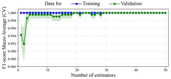
Figure 7.
Validation curve for the n_estimators hyperparameter in the ET classifier. The plot shows macro-averaged F1-scores from a stratified 5-fold cross-validation. The blue curve represents training performance, and the green curve shows validation performance, with the green shaded area representing ±1 Std. Dev. of the validation scores across the folds. Validation performance improves rapidly and then stabilizes near 1.0 at ∼29 trees, indicating that further increases in model complexity do not enhance generalization.
To evaluate the statistical significance of the ET classifier’s performance, the results of a permutation test are depicted in Figure 8. The test evaluates the null hypothesis (): there is no relationship between the features and the labels, and any observed performance arises purely by chance. To assess this, 100 random permutations of the training labels were performed, each followed by 5-fold cross-validation. The resulting F1-scores form an empirical distribution of model performance under random label conditions. The observed F1-score, obtained using the true labels, is 1.0 (blue dashed line), and falls far outside the range of scores produced under . The corresponding p-value is 0.0099, indicating that such a high score would be expected by chance in fewer than 1% of the permutations.
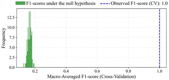
Figure 8.
Permutation test for evaluating the statistical significance of the classifier’s performance. The null hypothesis () states that there is no real relationship between features and labels. The histogram displays macro-averaged F1-scores from 100 random permutations of the training labels, each evaluated using 5-fold cross-validation. The observed F1-score (1.0) obtained with the true labels lies far outside the range of scores produced under . The p-value of 0.0099 supports the rejection of , indicating that the model’s performance is statistically significant.
4. Discussion
The findings of this study clearly demonstrate that the efficacy of combining spectral derivative preprocessing with ML algorithms is effective for classifying six common industrial plastic polymers (PET, HDPE, PVC, LDPE, PP, and PS) based on their FTIR spectra acquired at a resolution of 8 . The thorough methodology, which includes an initial data split to prevent bias and repeated, stratified cross-validation for choosing models, offers strong evidence for the robustness and broad applicability of the results.
Among the evaluated preprocessing strategies, the first spectral derivative, calculated using the Savitzky–Golay filter (21-point window, second-order polynomial), proved to be a particularly effective transformation. Its impact was most significant on the MLP classifier, which performed poorly on raw data (zeroth derivative) with a mean F1-score in cross-validation of ∼0.446. However, this improved dramatically to nearly perfect levels (F1 > 0.999) when the first or second derivative was applied. This finding emphasizes the sensitivity of neural networks to input feature representations and confirms the importance of spectral derivatives in reducing baseline distortions while enhancing distinctive spectral features.
For the other classifiers (ET, LDA, and RF), which already exhibited a strong performance with unprocessed spectra, the first derivative further improved their accuracy and decreased variability (lower standard deviation across cross-validation folds). Notably, the ET classifier reached its best performance with the first derivative, suggesting that the additional complexity of the second derivative was unnecessary. Although the second derivative also produced good results, it did not consistently outperform the first and sometimes slightly reduced performance due to possible over-smoothing.
The ET classifier, combined with the first derivative, was identified as the optimal model. It achieved an average F1-score of 0.99995 (±0.00033) during cross-validation and reached perfect classification (1.0) across all evaluated metrics: Accuracy, F1-score, Cohen’s Kappa, and Matthews Correlation Coefficient) on the independent test set. This outstanding result demonstrates the model’s ability for accurate prediction and its robustness under previously unseen data conditions. LDA also produced excellent results, especially when used with the first or second derivative, consistently achieving F1-scores above 0.9998. This indicates that the application of derivatives makes the polymer classes nearly or entirely linearly separable in the transformed feature space. The RF and MLP models, when combined with derivative preprocessing, were also highly competitive, generating average F1-scores exceeding 0.999. In contrast, the SVC, although still performing well (F1 score > 0.988 with the first derivative), was outperformed by the other models and showed greater variability and sensitivity to the choice of derivative.
This study’s key methodological strength is its strict train-test separation, with the final evaluation set used only after all of the model development concluded. The fact that the ET model achieved outstanding results during repeated cross-validation (10 repetitions of 5 folds) and also performed flawlessly on the test set boosts confidence in its ability to extract meaningful and discriminative spectral features. The very low standard deviation in F1-score (±0.00033) further confirms its consistency and predictive dependability.
Achieving perfect classification on the test set using FTIR spectra at a resolution of 8 is a significant achievement. It indicates that, under controlled conditions with relatively pure polymer samples, the classification task is quite manageable with proper preprocessing and model choice. However, these results should be viewed in context: real-world applications often involve more complex samples, such as polymer blends, degraded materials, additives, or spectra collected with different noise levels and instruments. These factors could affect model performance and how well the results generalize. Interestingly, the successful classification at 8 resolution implies this setting might be adequate or even better than higher resolutions such as 4 . The latter could introduce unnecessary noise or redundant information without offering significant improvements in performance.
From a practical perspective, this work offers several key contributions. First, it provides clear methodological guidance on preprocessing, demonstrating the value of applying the first spectral derivative in FTIR-based plastic analysis with ML, and proposes a rigorous protocol for model selection and validation that can be generalized to similar spectral classification tasks. Second, it identifies a set of highly effective classifiers, most notably ET and LDA, which not only deliver excellent predictive performance and stability, but also, in the case of ET and RF, demonstrate computational efficiency during training, as shown in Figure 4. Third, the study emphasizes the importance of rigorous validation practices by implementing a strict separation between the development and final evaluation phases, which enhances the reliability and generalizability of the reported results. Finally, the high levels of accuracy observed, along with the flawless classification of test data, suggest great potential for real-world application in automated systems for plastic polymer identification, including industrial recycling lines, quality control workflows, and environmental research efforts such as microplastic detection and monitoring.
As shown in Figure 7, the learning curve indicates that the ET classifier achieves a balanced fit, with no signs of underfitting or overfitting. In early stages (200–600 samples), the gap between training and validation indicates room for learning, but as more data are added, this gap closes. Around 840 training samples (∼140 per class), the model reaches maximum generalization capacity, with nearly perfect F1-scores in both training and cross-validation. The reduced variance among cross-validation repetitions further supports this stability. These results suggest that the spectral classes are highly separable and that the combination of Savitzky–Golay preprocessing and the ET model is particularly effective for this FTIR-based classification task
The results depicted in Figure 7 demonstrate the ET classifier’s capacity for efficient and stable learning across increasing model complexity. Even with fewer than 5 estimators, the model exhibits high predictive scores. However, from around 19 estimators onward, the validation performance saturates at 1.0 without variance, indicating strong generalization and resilience. No signs of overfitting are observed, as training and validation scores remain closely aligned throughout. A practical balance between performance and computational efficiency is reached around 30 estimators.
Evidence from the permutation analysis in Figure 8 strongly suggests that the ET classifier is learning genuine patterns present in the data rather than artifacts of noise. The null hypothesis (), which states that the features and labels are statistically independent and that model performance arises by chance, was tested using 100 random label permutations, each followed by 5-fold cross-validation. The resulting F1-scores under random label assignments fell within a narrow and low range (approximately 0.15–0.25), as expected when no true relationship exists. In contrast, the observed F1-score with the true labels was 1.0, a clear outlier with respect to these randomized outcomes. The associated p-value of 0.00990 leads to the rejection of at the 1% significance level, confirming that the classifier’s predictive performance is not attributable to random chance. This conclusion is further supported by a perfect Kappa score of 1.0, indicating complete agreement beyond chance expectations.
4.1. Comparison with Previous Studies
The combination of spectroscopy with ML for plastic polymer identification is a rapidly evolving field, with numerous studies demonstrating high classification accuracy across various techniques such as Near-Infrared (NIR), Mid-Infrared (MIR), and Raman spectroscopy.
Several studies demonstrate the impact of sophisticated spectral preprocessing to achieve state-of-the-art results. For instance, Zhu et al. [42] applied NIR spectroscopy to aged polypropylene, finding that a second-derivative spectral transformation combined with a linear SVC achieved 99% accuracy in distinguishing aging stages. Similarly, Stavinski et al. [29] utilized MIR spectroscopy on post-consumer plastics, achieving 100% accuracy with an RF model by focusing on “clean” spectral regions (C–H stretching and fingerprint regions) devoid of additive interference. The significance of a customized preprocessing pipeline was emphasized by Sutliff et al. [43], who systematically optimized over 12,000 preprocessing and classifier combinations to distinguish polyolefin species, identifying multiple workflows that achieved over 95% precision.
Our findings are in strong alignment with these studies, confirming that derivative preprocessing is decisive. However, our work identifies a specific and effective pipeline: a first-derivative Savitzky-Golay filter (using a 2nd-order polynomial and a 21-point window) paired with an ET classifier, which achieved a perfect classification score across all six polymer types. This result matches the accuracy reported by Stavinski et al. [29], but does so using the full FTIR spectral range.
Other research has focused on the challenges posed by data acquisition and sample heterogeneity. van Hoorn et al. [44] compared portable NIR spectrometers against a high-resolution benchtop instrument for classifying six common plastics, noting a significant drop in accuracy from ∼97% with the high-resolution device to as low as 70% with one of the portable units. This highlights the sensitivity of ML models to spectral data quality. Furthermore, Pocheville et al. [45] tackled the challenging task of sorting real-world waste from electronic equipment (WEEE) using Raman spectroscopy. Even with advanced Discriminant Analysis (DA) models, the separation purity for PS and ABS plastics from mixed, real-world samples reached approximately 80%, underscoring the performance gap between well-characterized laboratory samples and complex, contaminated waste streams.
In this context, our study introduces a clear and rigorous methodology that achieves an outstanding performance on a foundational six-polymer dataset. Although prior research has shown that high accuracies can be obtained with a variety of spectral techniques and ML models, our findings identify a particularly effective and computationally efficient configuration (ET combined with a first derivative) that attains a perfect score. This establishes a strong baseline and validates a reproducible methodological pipeline. Building on this, and in light of the challenges highlighted by van Hoorn et al. [44] and Pocheville et al. [45], the next logical step is to evaluate the robustness of this optimized pipeline on more complex, real-world post-consumer waste samples.
4.2. The Model in the Context of Existing Spectroscopic Tools
Commercial software for polymer identification via FTIR spectroscopy is predominantly engineered around spectral library matching. This technique involves comparing a sample’s spectrum against a database composed of pristine reference materials [46]. Although this method is effective for pure, well-characterized samples, its performance falters when analyzing real-world materials whose spectral signatures have been altered by environmental aging, additives, or contamination [47]. Research indicates that the primary metric for this method, the Hit Quality Index (HQI), does not reliably correlate with identification accuracy, which can range from as low as 64.1% to 98% [46]. In contrast, ML models provide a more robust alternative by learning to discern the fundamental patterns inherent to polymer classes, thereby achieving classification accuracies that consistently reach 99.5% [18]. This has led to the conclusion that ML methodologies afford a more ”precise and unambiguous identification” when compared to conventional spectral matching algorithms [47].
It is important to emphasize that this work does not seek to replace high-resolution FTIR systems or expert-driven spectral libraries, but rather to provide a complementary, automated pathway for polymer identification (particularly valuable in resource-constrained, high-throughput, or field-deployable scenarios). The demonstrated robustness at 8 suggests that such ML-enhanced pipelines can maintain high accuracy even when spectral fidelity is compromised, thereby opening the door for integration with portable, educational, or industrial-grade instruments. Future work will explore direct deployment on such platforms, as well as hybrid approaches combining database matching with ML-based feature learning.
This complementary function is especially critical due to the expanding use of portable and low-cost spectrometers, which inherently generate data with lower resolution and inferior signal-to-noise ratios [48]. Comparative studies have documented a significant decline in classification accuracy from 97% on laboratory instruments to as low as 70% on certain handheld devices [44]. The validity of the proposed hybrid approach is corroborated by commercial software, such as the solution from Jasco, which already employs a two-stage model. This model first applies ML for broad classification before using a library search for refinement, a process proven effective for degraded plastics [49]. Furthermore, the development of advanced deep learning methods to computationally reconstruct low-quality spectra reinforces the potential to achieve high accuracy even with compromised data [50].
4.3. Limitations and Future Work
While the results of this study are highly promising, some limitations should be acknowledged, offering directions for future research. First, although a resolution of 8 was selected due to its strong performance and computational efficiency, a formal and systematic comparison with higher-resolution spectra (such as 4 ) using the same robust methodology could provide deeper insights into the potential trade-offs between resolution, model accuracy, and computational cost. It should be noted that the FTIR spectra used in this study are not simulations but publicly available, real-world data. The choice of this relatively low resolution was deliberate, aimed at rigorously testing the robustness, generalization, and efficacy of our machine learning models on data that can be more challenging to find inherent patterns in than higher-resolution laboratory spectra.
Another important consideration involves hyperparameter optimization. In this work, models were evaluated using default configurations from the Scikit-learn library, with fixed random seeds to ensure reproducibility. While this approach sufficed to reveal general performance trends, conducting exhaustive or automated hyperparameter tuning, particularly for SVC and MLP, could yield further performance improvements or optimize tree-based models for specific use cases.
Regarding data complexity, the spectral data analyzed in this study corresponded to relatively pure samples of each plastic polymer. However, real-world scenarios often involve more complex conditions, including degraded materials, additives, contaminants, or polymer blends. Evaluating the trained models on such heterogeneous and noisy samples is a crucial step to verify their applicability in practical industrial or environmental settings.
Additionally, although the classification performance was the primary focus, model interpretability was not explored in this study. Applying techniques such as feature importance analysis for tree-based models or more advanced interpretability frameworks like SHapley Addictive exPlanations (SHAP) or Local Interpretable Model-agnostic Explanations (LIME) can provide valuable information on which spectral regions contribute most to classification. This, in turn, could inform future dimensionality reduction strategies or offer chemically meaningful interpretations of model decisions.
Finally, it is important to recognize that, while FFT-based filtering remains a strong tool for reducing instrumental noise, its use as a post-acquisition preprocessing step for ML classification (especially when combined with derivative transformations) is still not well explored. Future research will explore hybrid pipelines (for example, FFT → Inverse FFT → Savitzky–Golay derivatives → ML) to see if combining noise reduction and feature enhancement can better improve model generalization, particularly in field-deployed or low-resolution FTIR systems.
5. Conclusions
This study demonstrated that the integration of spectral derivative preprocessing, specifically the first derivative calculated via the Savitzky–Golay filter, with machine learning models enables highly accurate classification of primary industrial plastics (PET, PP, HDPE, LDPE, PS, and PVC) using FTIR spectroscopy at a resolution of 8 .
Among the evaluated models, the combination of the first derivative with the Extremely Randomized Trees (ETs) classifier consistently achieved superior performance, culminating in perfect classification on the held-out test set across all evaluation metrics, as reported in Table 4. This result was supported by an exceptionally high and stable average F1-score (0.99995 ± 0.00033) observed in a rigorous repeated and stratified cross-validation procedure (Table 3), confirming both the reliability and generalizability of the proposed approach. The LDA model also resulted as a highly effective alternative when used with the first or second spectral derivative, indicating that the preprocessing step rendered the polymer classes nearly linearly separable in the transformed feature space. Additionally, the study revealed that models such as MLP, which initially performed poorly on raw spectral data, experienced significant performance gains when combined with derivative-based preprocessing.
Overall, the findings emphasize the importance of carefully choosing and adjusting spectral preprocessing methods to suit the data and the learning model. The rigorous approach taken, including strict separation between training and testing phases, repeated cross-validation, and the use of a hold-out test set, strongly supports the results reported. This study validates the combination of first-derivative preprocessing with ET as an excellent solution for FTIR-based plastic classification. Also, it reinforces the broader potential of machine learning approaches for developing automated, high-precision, and efficient tools in applications such as industrial quality control, plastic waste management, and environmental monitoring of plastic pollution.
Additionally, our results confirm that spectral derivatives, when combined with suitable machine learning models, can achieve a high classification accuracy even under less-than-ideal spectral conditions (such as 8 resolution), which are common in field-deployable or budget-limited FTIR systems. Far from replacing existing analytical workflows, this method provides a scalable, automated supplement, expanding the application of FTIR-based polymer identification into new practical domains.
Future research should investigate the transferability of these models to more complex, real-world samples and alternative acquisition conditions to expand their practical relevance and deployment further.
Author Contributions
Conceptualization, O.R.-M., R.A.-E. and E.E.G.-G.; methodology, O.R.-M. and R.A.G.-H.; software, O.R.-M.; validation, O.R.-M., E.E.G.-G. and R.A.G.-H.; formal analysis, O.R.-M., R.A.-E. and R.A.G.-H.; investigation, O.R.-M.; resources, E.E.G.-G. and A.A.F.-F.; data curation, O.R.-M.; writing—original draft preparation, O.R.-M.; writing—review and editing, O.R.-M. and E.E.G.-G.; visualization, O.R.-M.; supervision, E.E.G.-G. and A.A.F.-F.; project administration, O.R.-M. and E.E.G.-G. All authors have read and agreed to the published version of the manuscript.
Funding
This research was partially funded by the Tecnológico Nacional de México/Instituto Tecnológico de Toluca under Project 19665.24P. Additional support was provided by SECIHTI through a doctoral fellowship granted to O.R-M. (CVU No. 932933, Grant No. 4043887).
Data Availability Statement
The original dataset analyzed during the current study was published by Villegas-Camacho et al. [19] and is publicly available.
Acknowledgments
The authors acknowledge the creators of the public dataset used in this study. Also, to Universidad Autónoma del Estado de México/Unidad Académica Profesional Tianguistenco for the opportunity to pursue doctoral studies.
Conflicts of Interest
The authors declare no conflicts of interest.
References
- OECD. Global Plastics Outlook: Economic Drivers, Environmental Impacts and Policy Options; OECD: Paris, France, 2022. [Google Scholar] [CrossRef]
- Song, J.; Wang, C.; Li, G. Defining Primary and Secondary Microplastics: A Connotation Analysis. ACS EST Water 2024, 4, 2330–2332. [Google Scholar] [CrossRef]
- McHale, M.E.; Sheehan, K.L. Bioaccumulation, transfer, and impacts of microplastics in aquatic food chains. J. Environ. Expo. Assess. 2024, 3, 15. [Google Scholar] [CrossRef]
- Fakayode, S.O.; Mehari, T.F.; Narcisse, V.E.F.; Grant, C.; Taylor, M.E.; Baker, G.A.; Siraj, N.; Bashiru, M.; Denmark, I.; Oyebade, A.; et al. Microplastics: Challenges, toxicity, spectroscopic and real-time detection methods. Appl. Spectrosc. Rev. 2024, 59, 1183–1277. [Google Scholar] [CrossRef]
- Enyoh, C.E.; Wang, Q. Automated Classification of Undegraded and Aged Polyethylene Terephthalate Microplastics from ATR-FTIR Spectroscopy using Machine Learning Algorithms. J. Polym. Environ. 2023, 32, 4143–4158. [Google Scholar] [CrossRef]
- Kedzierski, M.; Falcou-Préfol, M.; Kerros, M.E.; Henry, M.; Pedrotti, M.L.; Bruzaud, S. A machine learning algorithm for high throughput identification of FTIR spectra: Application on microplastics collected in the Mediterranean Sea. Chemosphere 2019, 234, 242–251. [Google Scholar] [CrossRef]
- Moses, S.R.; Roscher, L.; Primpke, S.; Hufnagl, B.; Löder, M.G.J.; Gerdts, G.; Laforsch, C. Comparison of two rapid automated analysis tools for large FTIR microplastic datasets. Anal. Bioanal. Chem. 2023, 415, 2975–2987. [Google Scholar] [CrossRef]
- Almanifi, O.R.A.; Ng, J.K.; Majeed, A.P.P.A. The Classification of FTIR Plastic Bag Spectra via Label Spreading and Stacking. Mekatronika 2021, 3, 70–76. [Google Scholar] [CrossRef]
- Khanam, M.M.; Uddin, M.K.; Kazi, J.U. Advances in machine learning for the detection and characterization of microplastics in the environment. Front. Environ. Sci. 2025, 13, 1573579. [Google Scholar] [CrossRef]
- Villegas-Camacho, O.; Francisco-Valencia, I.; Alejo-Eleuterio, R.; Granda-Gutiérrez, E.E.; Martínez-Gallegos, S.; Villanueva-Vásquez, D. FTIR-Based Microplastic Classification: A Comprehensive Study on Normalization and ML Techniques. Recycling 2025, 10, 46. [Google Scholar] [CrossRef]
- Shin, J.; Kim, D.C.; Cho, Y.; Yang, M.; Cho, W.J. A Preprocessing Technique Using Diffuse Reflectance Spectroscopy to Predict the Soil Properties of Paddy Fields in Korea. Appl. Sci. 2024, 14, 4673. [Google Scholar] [CrossRef]
- Helin, R.; Indahl, U.G.; Tomic, O.; Liland, K.H. On the possible benefits of deep learning for spectral preprocessing. J. Chemom. 2022, 36, e3374. [Google Scholar] [CrossRef]
- Delwiche, S.R.; Reeves, J.B. A Graphical Method to Evaluate Spectral Preprocessing in Multivariate Regression Calibrations: Example with Savitzky—Golay Filters and Partial Least Squares Regression. Appl. Spectrosc. 2010, 64, 73–82. [Google Scholar] [CrossRef]
- Zheng, C.; Liu, H.; Li, J.; Wang, Y. Identification and crude protein prediction of porcini mushrooms via deep learning-assisted FTIR fingerprinting. LWT 2024, 213, 117101. [Google Scholar] [CrossRef]
- Sitorus, A.; Muslih, M.; Cebro, I.S.; Bulan, R. Dataset of adulteration with water in coconut milk using FTIR spectroscopy. Data Brief 2021, 36, 107058. [Google Scholar] [CrossRef]
- Garg, S.; Sharma, A.; Sharma, V. Geographical profiling of wood samples via ATR-FTIR spectroscopy and machine learning algorithms: Application in wood forensics. Forensic Sci. Int. Rep. 2024, 10, 100377. [Google Scholar] [CrossRef]
- Liu, Y.; Yao, W.; Qin, F.; Zhou, L.; Zheng, Y. Spectral Classification of Large-Scale Blended (Micro)Plastics Using FT-IR Raw Spectra and Image-Based Machine Learning. Environ. Sci. Technol. 2023, 57, 6656–6663. [Google Scholar] [CrossRef] [PubMed]
- Tian, X.; Beén, F.; Sun, Y.; van Thienen, P.; Bäuerlein, P.S. Identification of Polymers with a Small Data Set of Mid-infrared Spectra: A Comparison between Machine Learning and Deep Learning Models. Environ. Sci. Technol. Lett. 2023, 10, 1030–1035. [Google Scholar] [CrossRef]
- Villegas-Camacho, O.; Alejo-Eleuterio, R.; Francisco-Valencia, I.; Granda-Gutiérrez, E.; Martínez-Gallegos, S.; Illescas, J. FTIR-Plastics: A Fourier Transform Infrared Spectroscopy dataset for the six most prevalent industrial plastic polymers. Data Brief 2024, 55, 110612. [Google Scholar] [CrossRef] [PubMed]
- Fadlelmoula, A.; Catarino, S.O.; Minas, G.; Carvalho, V. A Review of Machine Learning Methods Recently Applied to FTIR Spectroscopy Data for the Analysis of Human Blood Cells. Micromachines 2023, 14, 1145. [Google Scholar] [CrossRef]
- Neo, E.R.K.; Low, J.S.C.; Goodship, V.; Debattista, K. Deep learning for chemometric analysis of plastic spectral data from infrared and Raman databases. Resour. Conserv. Recycl. 2023, 188, 106718. [Google Scholar] [CrossRef]
- López, O.A.M.; López, A.M.; Crossa, J. Fundamentals of Artificial Neural Networks and Deep Learning. In Multivariate Statistical Machine Learning Methods for Genomic Prediction; Springer International Publishing: Berlin/Heidelberg, Germany, 2022; pp. 379–425. [Google Scholar] [CrossRef]
- Martinez-Hernandez, U.; West, G.; Assaf, T. Low-Cost Recognition of Plastic Waste Using Deep Learning and a Multi-Spectral Near-Infrared Sensor. Sensors 2024, 24, 2821. [Google Scholar] [CrossRef]
- Qu, L.; Pei, Y. A Comprehensive Review on Discriminant Analysis for Addressing Challenges of Class-Level Limitations, Small Sample Size, and Robustness. Processes 2024, 12, 1382. [Google Scholar] [CrossRef]
- Probst, P.; Wright, M.; Boulesteix, A.L. Hyperparameters and Tuning Strategies for Random Forest. WIREs Data Min. Knowl. Discov. 2019, 9, e1301. [Google Scholar] [CrossRef]
- Ren, Y.; Zhu, X.; Bai, K.; Zhang, R. A New Random Forest Ensemble of Intuitionistic Fuzzy Decision Trees. IEEE Trans. Fuzzy Syst. 2024, 32, 783–797. [Google Scholar] [CrossRef]
- Geurts, P.; Ernst, D.; Wehenkel, L. Extremely randomized trees. Mach. Learn. 2006, 63, 3–42. [Google Scholar] [CrossRef]
- Amaya-Tejera, N.; Gamarra, M.; Vélez, J.I.; Zurek, E. A distance-based kernel for classification via Support Vector Machines. Front. Artif. Intell. 2024, 7, 1287875. [Google Scholar] [CrossRef]
- Stavinski, N.; Maheshkar, V.; Thomas, S.; Dantu, K.; Velarde, L. Mid-infrared spectroscopy and machine learning for postconsumer plastics recycling. Environ. Sci. Adv. 2023, 2, 1099–1109. [Google Scholar] [CrossRef]
- Villarim, M.R.; Villarim, A.W.R.; Gazziro, M.; Cavallari, M.R.; Belfort, D.R.; Junior, O.H.A. Computational Tool for Curve Smoothing Methods Analysis and Surface Plasmon Resonance Biosensor Characterization. Inventions 2025, 10, 31. [Google Scholar] [CrossRef]
- Zimmermann, B.; Kohler, A. Optimizing Savitzky–Golay Parameters for Improving Spectral Resolution and Quantification in Infrared Spectroscopy. Appl. Spectrosc. 2013, 67, 892–902. [Google Scholar] [CrossRef]
- Sadeghi, M.; Behnia, F. Optimum window length of Savitzky-Golay filters with arbitrary order. arXiv 2018, arXiv:1808.10489. [Google Scholar]
- Markoulidakis, I.; Rallis, I.; Georgoulas, I.; Kopsiaftis, G.; Doulamis, A.; Doulamis, N. Multiclass Confusion Matrix Reduction Method and Its Application on Net Promoter Score Classification Problem. Technologies 2021, 9, 81. [Google Scholar] [CrossRef]
- Rainio, O.; Teuho, J.; Klén, R. Evaluation metrics and statistical tests for machine learning. Sci. Rep. 2024, 14, 6086. [Google Scholar] [CrossRef]
- Chicco, D.; Jurman, G. The Matthews correlation coefficient (MCC) should replace the ROC AUC as the standard metric for assessing binary classification. BioData Min. 2023, 16, 4. [Google Scholar] [CrossRef]
- Alpaydin, E. Introduction to Machine Learning, 4th ed.; MIT Press: Cambridge, MA, USA, 2020. [Google Scholar]
- Python Software Foundation. Python Language Reference, version 3.13.3; Python Software Foundation: Beaverton, OR, USA, 2025. Available online: https://docs.python.org/3.13/reference/ (accessed on 10 August 2025).
- Pedregosa, F.; Varoquaux, G.; Gramfort, A.; Michel, V.; Thirion, B.; Grisel, O.; Blondel, M.; Prettenhofer, P.; Weiss, R.; Dubourg, V.; et al. Scikit-learn: Machine Learning in Python. J. Mach. Learn. Res. 2011, 12, 2825–2830. [Google Scholar]
- McKinney, W. Python for Data Analysis: Data Wrangling with Pandas, Numpy, and Jupyter; O’Reilly Media, Inc.: Sebastopol, CA, USA, 2022. [Google Scholar]
- Harris, C.R.; Millman, K.J.; van der Walt, S.J.; Gommers, R.; Virtanen, P.; Cournapeau, D.; Wieser, E.; Taylor, J.; Berg, S.; Smith, N.J.; et al. Array programming with NumPy. Nature 2020, 585, 357–362. [Google Scholar] [CrossRef]
- Virtanen, P.; Gommers, R.; Oliphant, T.E.; Haberland, M.; Reddy, T.; Cournapeau, D.; Burovski, E.; Peterson, P.; Weckesser, W.; Bright, J.; et al. SciPy 1.0: Fundamental Algorithms for Scientific Computing in Python. Nat. Methods 2020, 17, 261–272. [Google Scholar] [CrossRef]
- Zhu, K.; Wu, D.; Yang, S.; Cao, C.; Zhou, W.; Qian, Q.; Chen, Q. Identification of Aged Polypropylene with Machine Learning and Near–Infrared Spectroscopy for Improved Recycling. Polymers 2025, 17, 700. [Google Scholar] [CrossRef]
- Sutliff, B.P.; Beaucage, P.A.; Audus, D.J.; Orski, S.V.; Martin, T.B. Sorting polyolefins with near-infrared spectroscopy: Identification of optimal data analysis pipelines and machine learning classifiers. Digit. Discov. 2024, 3, 2341–2355. [Google Scholar] [CrossRef]
- van Hoorn, H.; Pourmohammadi, F.; de Leeuw, A.W.; Vasulkar, A.; de Vos, J.; van den Berg, S. Machine Learning-Based Identification of Plastic Types Using Handheld Spectrometers. Sensors 2025, 25, 3777. [Google Scholar] [CrossRef] [PubMed]
- Pocheville, A.; Uria, I.; España, P.; Arnaiz, S. Raman spectroscopy integrated with machine learning techniques to improve industrial sorting of Waste Electric and Electronic Equipment (WEEE) plastics. J. Environ. Manag. 2025, 373, 123897. [Google Scholar] [CrossRef] [PubMed]
- Kozloski, R.; Cowger, W.; Arienzo, M.M. Moving toward automated µFTIR spectra matching for microplastic identification: Addressing false identifications and improving accuracy. Microplast. Nanoplast. 2024, 4, 27. [Google Scholar] [CrossRef]
- Prezgot, D.; Chen, M.; Leng, Y.; Gaburici, L.; Zou, S. Automated Machine-Learning-Driven Analysis of Microplastics by TGA-FTIR for Enhanced Identification and Quantification. Anal. Chem. 2025, 97, 8833–8840. [Google Scholar] [CrossRef] [PubMed]
- Said, M.; Amr, M.; Sabry, Y.M.; Khalil, D.A.; Wahba, A. Plastic sorting An Open-Source on MEMS FTIR spectral chemometrics sensing. In Optical Sensing and Detection VI; Berghmans, F., Mignani, A.G., Eds.; SPIE: Bellingham, WA, USA, 2020; Volume 11354, p. 22. [Google Scholar] [CrossRef]
- Group, J.G.S. Identification of Degraded Plastics Cross-Checking IR Spectra Using Machine Learning Classification and Library Search. 2025. Available online: https://www.jasco-global.com/solutions/identification-of-degraded-plastics-cross-checking-ir-spectra-using-machine-learning-classification-and-library-search/ (accessed on 18 September 2025).
- Brandt, J.; Mattsson, K.; Hassellöv, M. Deep Learning for Reconstructing Low-Quality FTIR and Raman Spectra—A Case Study in Microplastic Analyses. Anal. Chem. 2021, 93, 16360–16368. [Google Scholar] [CrossRef] [PubMed]
Disclaimer/Publisher’s Note: The statements, opinions and data contained in all publications are solely those of the individual author(s) and contributor(s) and not of MDPI and/or the editor(s). MDPI and/or the editor(s) disclaim responsibility for any injury to people or property resulting from any ideas, methods, instructions or products referred to in the content. |
© 2025 by the authors. Licensee MDPI, Basel, Switzerland. This article is an open access article distributed under the terms and conditions of the Creative Commons Attribution (CC BY) license (https://creativecommons.org/licenses/by/4.0/).