Article

Dimensionless Modelling of Bond-Based Peridynamic Models and Strategies for Enhancing Numerical Accuracy

1
School of Mechanical Engineering, Jiangsu University of Science and Technology, Zhenjiang 212100, China
2
School of Civil Engineering and Architecture, Jiangsu University of Science and Technology, Zhenjiang 212100, China
*
Author to whom correspondence should be addressed.
Modelling 2025, 6(3), 99; https://doi.org/10.3390/modelling6030099
Submission received: 23 July 2025 / Revised: 5 September 2025 / Accepted: 8 September 2025 / Published: 8 September 2025

Abstract

Peridynamics (PD) exhibits inherent advantages in solving solid mechanics problems involving strong discontinuities, such as crack propagation. However, the significant magnitude discrepancy between the micro-modulus and bond stretch in the nonlocal modelling, the extensive accumulation operations during nonlocal interaction integration, and the calculation methods for surface-correction coefficients can all introduce or amplify numerical errors, thereby reducing the confidence in numerical results. To address these sources of error and enhance the numerical accuracy of the PD models, this study derived a dimensionless bond-based PD formulation and proposed computational strategies to mitigate numerical errors during model implementation. The correctness of the dimensionless bond-based PD model was validated through investigating an elastic-wave propagation problem and a crack-branching problem, and comparing the numerical results with that from the finite-element method and the referenced literature. The effectiveness of the dimensionless model and the numerical strategies in enhancing numerical accuracy was verified through comparing the numerical performance of the model while investigating symmetrical mechanical problems under extreme computational conditions and load conditions. This study provides an effective modelling framework and numerical processing strategies for accurate computations in PD.

1. Introduction

Damage initiation and propagation in materials have long been challenging problems in computational mechanics, primarily due to the rationality of crack initiation criteria and the limited compatibility of conventional numerical methods, such as finite-element method (FEM) [1] and extended finite-element method (XFEM) [2], smooth particle hydrodynamics (SPH) [3], material point method (MPM) [4], and phase field method (PFM) [5], with strong discontinuities. The PD method [6,7] introduces nonlocal interactions, reformulating the governing equations of solid mechanics in integral form. The integral-form equations inherently accommodate strong discontinuities, such as cracks, without requiring additional treatments. PD has demonstrated extensive applicability, rapid development, and promising prospects [8]. However, the PD method exhibits computational inaccuracies in surface-correction factor calculations [9] and numerical integration processes [10]. In order to enhance the computational accuracy and result reliability, it is essential to mitigate error sources throughout both model formulation and implementation processes.
Numerical errors are inevitable when employing existing computational methods, such as FEM [11,12], finite volume method (FVM) [11,13,14], and mesh-free methods [15,16,17], to simulate physical processes. In these methods, as the gradients of physical quantities increase, such as problems involving strong shock waves or cracks [18], computational errors escalate. To mitigate this issue, typical approaches include increasing discretization density [19,20,21], adopting higher-order discretization schemes [22], and implementing specialized algorithms like the extended finite-element method (XFEM) [23] to counteract the decline in computational accuracy. However, these measures introduce difficulties in mathematical modelling, increased computational costs, and high-order oscillations in numerical solutions, failing to fundamentally address the issue of declining numerical accuracy. The integral formulation of nonlocal interactions in PD effectively accommodates large physical field gradients and even differential distortions. Therefore, it is imperative to conduct in-depth research on the limitations and numerical errors of the PD method.
The computational errors in the PD method primarily arise from mathematical modelling [24,25], discretization of the computational domain [26], organization of neighborhood members [27], determination of volume correction factors, and calculation of surface-correction factors. These errors can even lead to obvious inaccuracies in numerical simulations. For example, in a 2D symmetric model, numerical errors caused the crack to propagate asymmetrically [27]. In the modelling stage, the bond-based PD model has inherent Poisson’s ratio limitations [28]. For 2D models, the Poisson’s ratio is restricted to 1/3, while in 3D bond-based PD models, the Poisson’s ratio is constrained to 1/4. Additionally, in bond-based PD models, the micro-modulus of bonds typically reaches an order of magnitude of 1020, while the bond stretch is approximately 10−3. The multiplication of these two values can amplify the floating-point round-off error of the bond stretch [29]. Due to the inconsistency between the material point horizon and the discretized shape of the computational domain, the volumes of material point members located at horizon boundaries require correction [30], and the current correction methods remain relatively crude. The study of error sources in modelling and model implementation processes serves as an effective approach to enhance the numerical accuracy of PD models.
Dimensionless modelling holds significant importance in scientific research. The significance of dimensionless modelling lies in its ability to simplify complex processes by eliminating the influence of physical dimensions, thereby making mathematical analysis more concise [31]. In physical chemistry, dimensional analysis serves not only to verify the accuracy of equations but also to reveal new physical phenomena. The dimensionless approach can indeed reduce numerical computation errors [32,33,34,35]. By eliminating dimensional influences through standardized processing methods, it enhances calculation stability and convergence efficiency. This technique is particularly valuable in computational fluid dynamics (CFD), where dimensionless parameters like Reynolds number prevent floating-point overflow and maintain solution accuracy [36]. Moreover, dimensionless models provide fundamental support for similarity analysis of physical processes [37,38]. Based on similarity theory, both the implementation difficulty and cost of validation experiments in scientific research can be significantly reduced.
In this work, based on the original bond-based PD model, we established a dimensionless bond-based PD model. The work is organized as follows: The detailed establishment process of the dimensionless PD model and the computational methodology employed to solve the model are presented in Section 2. Section 3 primarily analyzes the error sources during model programming and computation, while proposing numerical strategies to suppress errors and enhance solution accuracy. The validation analysis of the dimensionless PD model and the effectiveness discussions of numerical strategies for computational accuracy enhancement are both addressed in Section 4. Finally, the work is concluded in Section 5.

2. Dimensionless Bond-Based PD Model

2.1. Bond-Based PD Model [4]

The basic equation for bond-based PD is given in Equation (1), which is used to define the motion of material points in the computational domain.
ρ u ¨ ( x , t ) = H ( x ) f ( x x , u u , t ) d V x + b ( x , t )
where ρ is the mass density, x is a material point in the neighborhood H ( x ) of material point x , u and u are, respectively, the displacement vector of material point x and x , u ¨ is the acceleration vector of material point x , d V x is the volume represented by material point x , b is the external body force vector, and f is the pairwise force density. The core of the bond-based PD model lies in the expression for the pairwise force density, whose magnitude is given by Equation (2).
f = c ( ξ ) s
where c ( ξ ) is the micro modulus function, which can be a constant or other types of expressions about the length of bond ξ in the referenced configuration, and s is the stretch of the bond, the specific expression of the bond stretch is given in Equation (3).
s = η + ξ ξ ξ
where η is the relative displacement between the two material points linked by bond ξ .
In this work, a constant micro modulus function c 0 given in Equation (4) for two-dimensional plane stress problems is utilized.
c 0 = 9   E π h δ 3
where E is the elastic modulus of the material, h is the thickness of the 2D problem, δ is the horizon of the PD neighborhood. In bond-based PD theory, damage and crack propagation are realized through bond breakage, which occurs when the bond stretch reaches the critical stretch. For plane stress problems, the expression for the critical stretch is given by Equation (5).
s 0 = 4 π G c 9 E δ
where G c is the fracture energy of the material.

2.2. Reference Variables

Among the seven fundamental SI base dimensions, those directly relevant to PD are: Length, time, mass, and temperature. These four units form the core dimensional basis for PD formulations. Among them, length and time define spatial discretization and temporal discretization. Mass appears in the density terms and temperature is critical for thermo-mechanical couplings. The four fundamental variables are labeled as: u 0 , m 0 , t 0 , and T 0 . Due to the dimensional independence of temperature and the models shown in Equations (1) and (2), this paper does not further discuss the nondimensionalization of temperature.
As shown in Equation (6), the reference length is u 0 and its specific form can be the discretization size of the domain, the neighborhood horizon, or the characteristic dimension of the structure, among others. Based on the definition of mass, the reference mass can be directly determined by multiplying the material density by the cube of the reference length, which is given in Equation (7). The reference time can be defined in terms of the reference length and velocity. Given that the solid wave speed plays a critical role in structural responses, as illustrated in Equation (8), the study defines the reference time based on the reference length and wave speed.
u 0 = u 0
m 0 = ρ u 0 3
t 0 = u 0 c W
where ρ is the mass density of the material, and c W = E ρ is the wave speed in the material.

2.3. Dimensionless Model

Based on the reference variables in Equations (6)–(8), the corresponding dimensionless displacement u ¯ , dimensionless mass m ¯ and dimensionless time t ¯ are, respectively, given in Equations (9)–(11).
u ¯ = u u 0
m ¯ = m m 0
t ¯ = t t 0
Based on the fundamental variables, derived variables related to the bond-based PD models are as follows:
The dimensionless velocity of the material points is given in Equation (12).
d u ¯ d t ¯ = 1 c W d u d t
The dimensionless acceleration of the material points is given in Equation (13).
u ¯ ¨ = d 2 u ¯ d t ¯ 2 = u 0 c W 2 d 2 u d t 2
The referenced volume is given in Equation (14), which can be derived from Equation (7).
V 0 = u 0 3
By substituting Equations (12)–(14) into Equation (1), Equation (15) can be derived.
u ¯ ¨ = H ( x ¯ ) f ¯ ( x ¯ x ¯ , u ¯ u ¯ , t ¯ ) d V ¯ x + b ¯ ( x ¯ , t ¯ )
where d V ¯ x = d V x V 0 is the dimensionless volume of the microelement represented by material point x , f ¯ is the dimensionless pairwise force density and b ¯ is the dimensionless body force, of which the detailed expressions of the magnitudes are, respectively, given in Equations (16) and (17).
f ¯ = c ¯ 0 s
b ¯ = u 0 E b
where c ¯ 0 is the dimensionless modulus of the constant modulus function. Based on Equation (4) and the dimensionless analysis, the dimensionless modulus is derived and expressed in Equation (18).
c ¯ 0 = u 0 4 E c 0 = 9 π u 0 h u 0 δ 3
According to Equations (16) and (18), the dimension of f ¯ is 1, indicating it is a dimensionless variable. Based on Equation (17), dimensional analysis reveals that the body force b ¯ is also dimensionless. Obviously, Equation (18) can also be applied to the nondimensionalization of other forms of micro modulus functions. Furthermore, the derivation reveals that the specific form of the length dimension directly determines the dimensionless forms of other variables. Therefore, the influences of length dimension on computational results should be further discussed in the subsequent analyses.

2.4. Numerical Scheme

The updating of the physical field in the work is implemented by using the explicit Velocity-Verlet scheme shown in Equations (19)–(21).
u ¯ ˙ n + 1 / 2 = u ¯ ˙ n + Δ t ¯ 2 u ¯ ¨ n
u ¯ n + 1 = u ¯ n + u ¯ ˙ n + 1 / 2 Δ t ¯
u ¯ ˙ n + 1 = u ¯ ˙ n + 1 / 2 + Δ t ¯ 2 u ¯ ¨ n + 1
where u ¯ ˙ represents the dimensionless velocity, and Δ t ¯ is the dimensionless time step size.

3. Error Sources and Numerical Strategies

3.1. Error Sources

In the calculations of PD models, the main sources of errors are as follows:
The first one is the storing of floating-point variables in computers. Consider a single-precision floating-point number represented in the 32-bit format as an example. According to the IEEE 754 standard [39], the first bit is the sign bit, the next 8 bits represent the exponent, and the remaining 23 bits store the mantissa. While theoretically there exists an infinite continuum of real numbers between any two numerical values, digital computers are fundamentally constrained by finite representation capabilities. When processing numerical data, computational systems must employ specific approximation strategies to handle values that cannot be precisely represented. This inherent limitation inevitably introduces rounding errors in digital computations. For example, computers cannot accurately represent the number 0.1.
The second source of error results from the extensive additive operations [40] involved in the numerical solution of the PD equation given in Equation (1) or (15). The integral in the PD equation is obtained through the accumulation of the product between the pairwise force and the corresponding volume element over the integration domain, specifically in the neighborhood of the studied material point. The error arises from the inconsistent ordering of material point lists, which leads to different summation sequences during numerical integration. Particularly for axisymmetric problems, such minor discrepancies can result in significant computational errors.
The third type of error comes from the calculation method of surface-correction factors in PD, which constitutes one of the primary computational errors in PD. In the calculation of the original surface-correction factors, a constant strain in a given direction was directly applied to the computational domain. By comparing the material point energy density obtained from PD calculations with the results from classical continuum mechanics theory, the surface-correction factors for each material point in different directions were ultimately determined. However, this approach may amplify the first type error, ultimately leading to reduced computational accuracy. Further explanation of this type of error source will be provided later through direct comparison of surface-correction factors obtained from different strategies.

3.2. Numerical Strategies

The first source of error given in Section 3.1 is fundamentally unavoidable in numerical computations, and their impact can only be mitigated by increasing floating-point precision through methods such as substituting double-precision numbers for single-precision ones. In PD theory, summation operations frequently occur, making errors inevitable. However, these computational errors originate from the order of summation. By implementing specific sorting rules to ensure consistent relative summation sequences within the neighborhood of each material point, uniform error magnitudes can be maintained across all material points. This approach controls the propagation of computational errors caused by inconsistent relative ordering of material points within neighborhoods, thereby preventing erroneous results. There are two aspects of strategies can be implemented to reduce the computational error.
The first strategy (S1) is to adjust the order of neighborhood material points within the horizon of a material point according to the method used for the yellow material points in Figure 1. This approach is suitable for solving symmetric problems. As shown in Figure 1, the 225th material point is denoted as P1, the 85th material point is denoted as P2, the 235th material point is denoted as Q1, and the 95th material point is denoted as Q2. In this problem, P1 and P2 are a pair of symmetrical material points, and Q1 and Q2 are another pair of symmetrical material points. For the symmetrical material points P1 and P2, the order of the neighborhood material point is consistent with the overall material point numbering order. Nevertheless, the orders of the neighborhood material point for Q1 and Q2 are symmetrical about the symmetry line of the problem. Obviously, this strategy further ensures the symmetry of the problem at the numerical processing level.
Considering the limitations of S1, which is mainly suitable for symmetric problems, the second strategy (S2) adopts a sorting method based on the distance between members in the neighborhood and the material point, which can reduce the calculation error to a certain extent. The intrinsic reason is that the pairwise force calculation involves the calculation of bond stretch. Take material point PR as an example, the serial numbers of material points within the neighborhood of material point PR, sorted by distance from point PR in ascending order, are shown in Figure 1. According to Equation (3), the denominator of the bond stretch formula is this distance. The effectiveness of this strategy will be further discussed in detail.
As shown in Figure 1, the material point PB is located near the boundary of the computational domain. Its horizon (2D) forms an incomplete circular region, which prevents the dynamic model from achieving force equilibrium. Therefore, corrections must be applied to material points near boundaries [41]. To resolve this issue, the conventional method for boundary-adjacent material points (e.g., material point k) involves enforcing strain energy density equivalence between PD W PD ( k ) and classical continuum mechanics formulations W CM ( k ) . This equivalence then determines the corresponding correction factors t r u i ( k ) for material point k according to Equation (22).
t r u i ( k ) = W CM ( k ) W PD ( k )
where in a 2D problem, the indices i = 1 and i = 2 correspond to the factors in x- and y-directions, respectively. To obtain the two correction factors, simple loading conditions are applied to the computational domain, enabling the theoretical derivation of the strain energy density in classical continuum mechanics. In this work, the computational domain is subjected to uniaxial stretch loadings in the x- and y-directions. Taking the x-direction correction factor as an example, the uniaxial stretching is achieved by applying a constant displacement gradient ε 0 along the x-direction of the computational domain. The displacement field of the computational domain under the loading can be expressed in the form of Equation (23).
u T = ε 0 x 0
where x is the horizontal coordinate of material points in the computational domain. Under dimensionless parameters, the strain energy density at material point k can be derived as W CM ( k ) = 9 16 ε 0 2 based on the loading condition and classical continuum mechanics theory. In contrast, the strain energy density from PD W PD ( k ) is numerically computed based on the displacement field defined in Equation (23), by accumulating the bond strain energy between material point k and all neighboring material points within its horizon. Typically, as shown in Figure 2a, the displacement field is first updated across the entire computational domain. Subsequently, the bond stretches within the neighborhood of material point k are calculated based on the displacement field, from which the total bond elastic potential energy of material point k is obtained. Due to variations in the x-coordinates across different material points, the amplification of the constant-strain storage errors differs spatially. This discrepancy propagates into variations in bond stretch calculation errors, ultimately inducing minor deviations in the computed correction factors. The third strategy (S3) is implemented to eliminate this error. While achieving the correction factor in the x-direction for material point k, as given in Equation (24), the core of this strategy involves applying the constant strain only within the horizon of the material point while computing the bond stretches, as shown in Figure 2b.
η x = ε 0 ξ x η y = 0
where ξ x is the initial bond length of bond ξ in the x-direction, η x and η y are the relative displacements of the two material points linked by the bond in the x-direction and y-direction, respectively. The surface-correction factor in the y-direction can be obtained through an analogous procedure.

4. Results and Discussions

In this section, the correctness of the dimensionless PD model in capturing elastic-wave and crack propagation is validated first. The primary objective of this validation is to demonstrate the validity of both the dimensionless PD model and its corresponding numerical implementation. Then, the effectiveness of the numerical strategies provided in Section 3.2 are discussed in detail.

4.1. Results

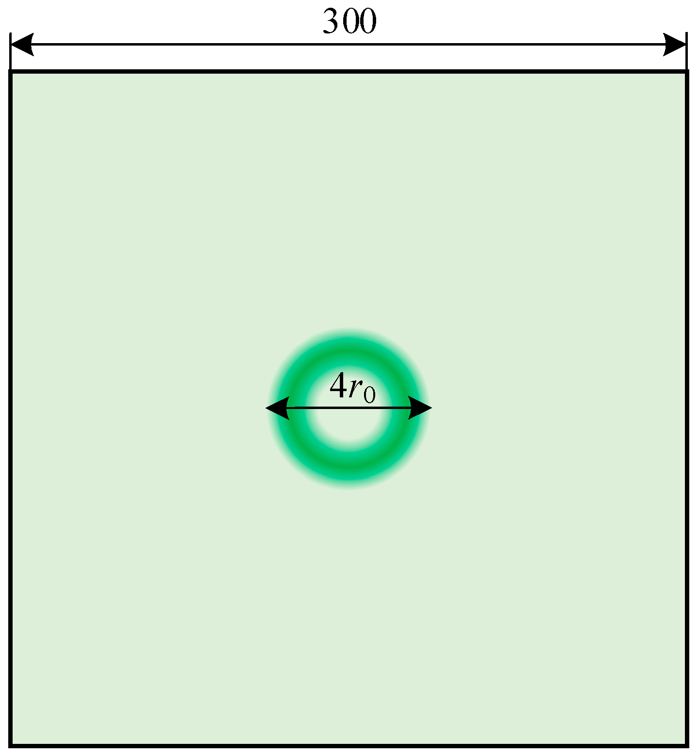
Similarly to the work [42], a square plate with initial displacement shown in Figure 3 was investigated to verify the correctness of the dimensionless model in capturing the development of two-dimensional elastic waves. As presented in work [42], the description of the nonlinear initial displacement is realized based on a precise discretization of the computational domain. Otherwise, it is impossible to accurately capture the nonlinear initial displacement distribution. In this work, a relatively simple nonlinear initial displacement is given in Equation (25) and illustrated in Figure 3.
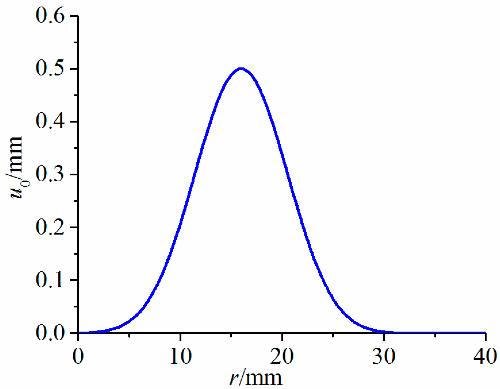
u ( r , t = 0 ) = A e B ( r r 0 ) 2 r 0 2 sin ( π r 2 r 0 ) r L c 0 r > L c
where A = 0.5 mm, B = 5.0, b = 2 mm, r0 = 16 mm, and the truncation distance Lc = 2 r0 = 32 mm. Detailed material properties are given in Table 1.
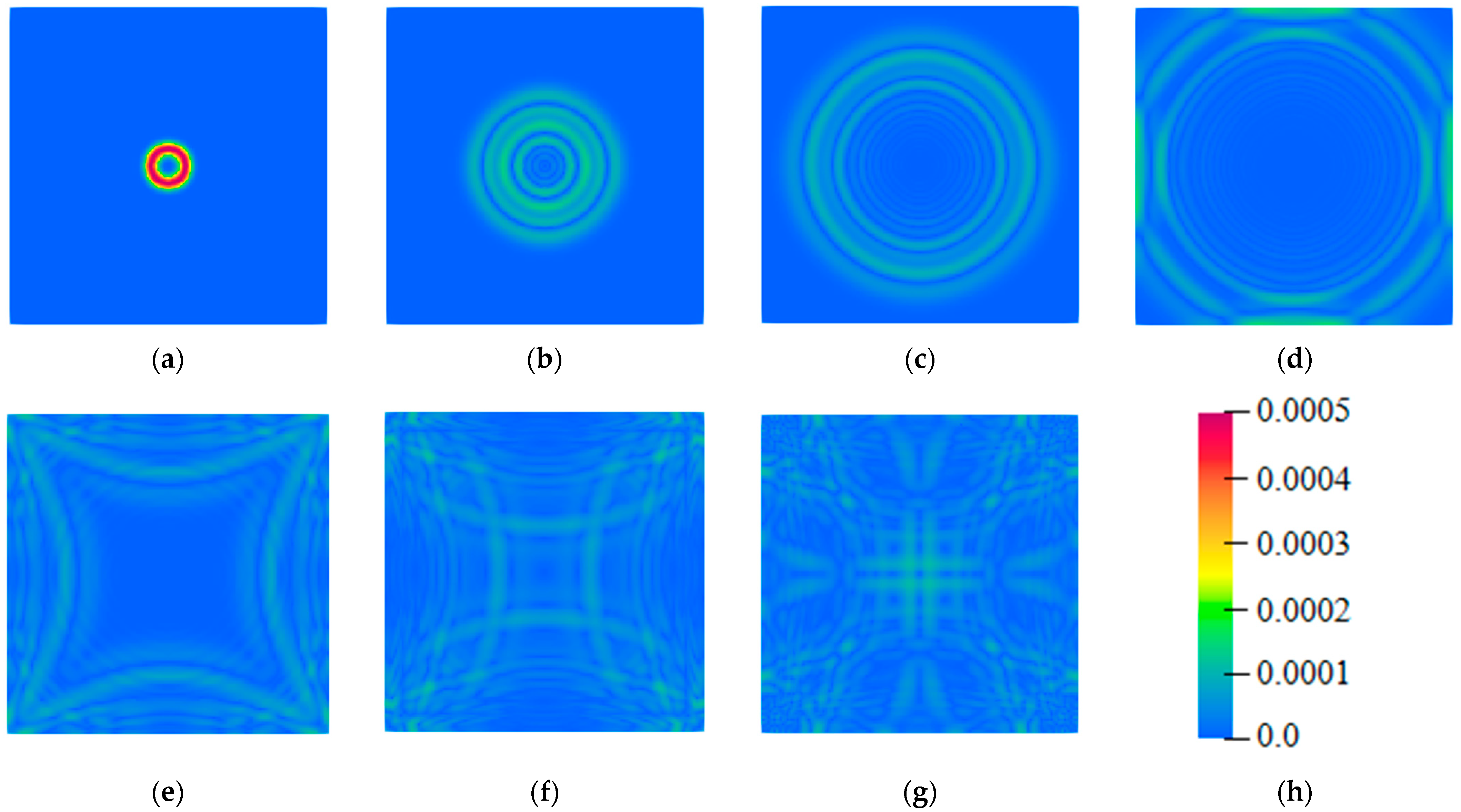
The specific distribution of the initial displacement is shown in Figure 4. The wave propagation in the square plate shown in Figure 3 was predicated by using both the dimensionless bond-based PD model and the finite-element method (FEM). The calculated histories of the elastic potential energy Es from the two numerical methods are compared in Figure 5. Obviously, the result from the dimensionless PD model agrees well with the result from the FEM, which can be reflected in the amplitude of the elastic potential energy and the moment of elastic potential energy fluctuations. The distributions of the displacement at different time from the dimensionless PD model are displayed in Figure 6, while the results from the FEM are provided in Figure 7. The computational results exhibit a high degree of consistency, particularly in terms of waveform morphology and the amplitude characteristics. The consistency of the calculation results reflects that the dimensionless PD model proposed in this paper can correctly capture the nonlinear elastic-wave propagation process.
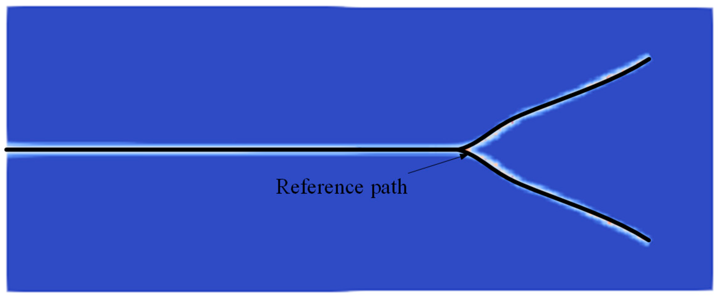
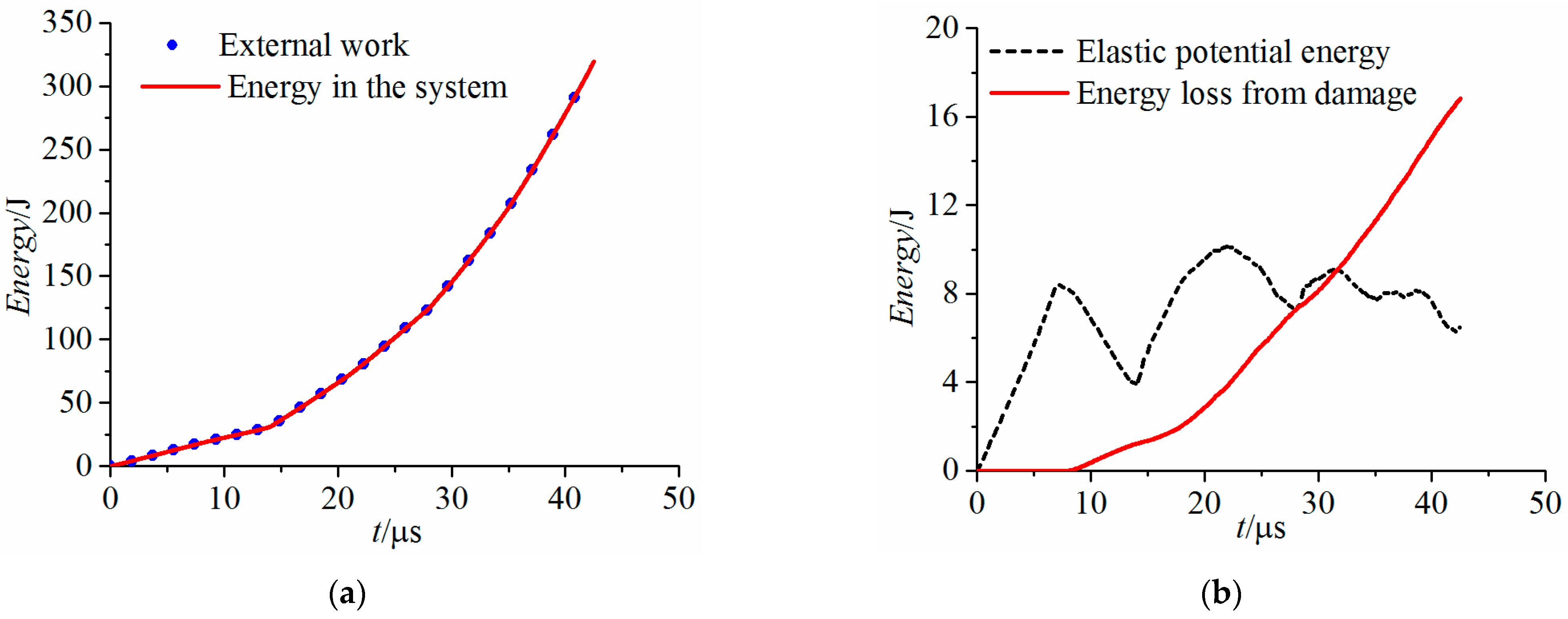
The correctness of the dimensionless model in capturing crack propagations is validated through the benchmark problem illustrated in Figure 8. A pre-notched plate made of Duran 50 glass is subjected to sudden traction stress on the upper and lower boundaries. Detailed dimensional parameters and material properties are given in Table 2. Based on the convergence study results of Bobaru [43], the plate is uniformly discretized by using a Δ of 0.25 mm. The length direction of the plate is divided into 400 equal parts, and the width direction of the plate is divided into 160 equal parts. The horizon δ = 1.00375 mm is used in the numerical simulation of the dimensionless PD model. Under a stress of 12.0 MPa, the predicted crack-branching path from the dimensionless PD model is compared with the crack path from Bobaru [43] in Figure 9. The energy conversion history is shown in Figure 10.
In Figure 9, the black lines denote the reference crack. The comparison of the results reveals that both the initiation points of the crack branching and the propagation trends of the crack path exhibit remarkable consistency. The observed consistency fully validates that the dimensionless PD model can accurately capture both damage initiation and crack propagation phenomena. In Figure 10a, the energy in the system includes the kinematic energy, the elastic potential energy and the energy loss caused by material damage. The external work WEx comes from the traction stress σ , which is calculated according to Equations (26) and (27).
W Ex ( n ) = i = 1 n Δ W Ex ( i )
Δ W Ex ( i ) = σ A j = 1 k ( v j i v j i 1 )
where n represents end of the nth time step, Δ W Ex ( i ) is the work increment of the ith time increment, A = h Δ is the area of acting surface of the stress on the volume represented by a material point, k is the number of material points needed to characterize the external stress, v j i is the vertical displacement of material j at the ith time step. According to Figure 10a, the consistency between the total energy in the system and the external work indicates the correctness of the computational model and program code. The correctness of the program code and the consistency of the predicted crack path with the reference path fully validate the correctness of the dimensionless PD model.
As illustrated in Figure 10b, there is a clear correlation between the elastic potential energy and the energy loss. Before the moment when the material damage starts, which is about 8.16 μs, the elastic potential energy increases rapidly. Once the material damage starts, part of the elastic potential energy is converted into the damage energy and forms new crack surfaces. Accordingly, the damage of the material, namely the breakage of bonds, will further affect the distribution of elastic potential energy in the system. Therefore, for a problem without initial strain, there is a significant interaction between the elastic potential energy and damage energy in the system.

4.2. Discussions

In this section, the effectiveness of the strategies for enhancing the accuracy of the numerical results was discussed. In the discussion, we chose to conduct the numerical simulations under more stringent conditions. The selected computational problem is the symmetric crack-branching propagation under a traction stress of 18 MPa, as shown in Figure 8. Additionally, in the calculations, real variables were stored in single-precision format.
Both S1 and S2 are designed to reorder material points within the neighborhood. To intuitively demonstrate the effect of S3, the first and the second strategies are considered together as a bundle. For brevity, the first and the second strategies are denoted as S12 in this work. Three cases shown in Table 3 were investigated.
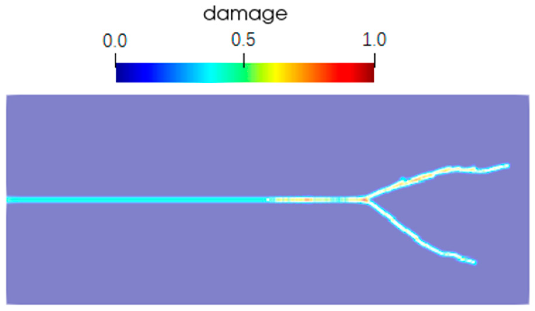
First, we compared the computational results from the dimensionless model and the original model. It should be noted that the numerical strategies proposed in Section 3.2 were employed in both models. The crack propagation paths at 35.0 μs obtained from the two models are compared in Figure 11. Under such extreme conditions, the dimensionless model demonstrated higher accuracy, and the symmetry of the computational results was significantly better than that from the original model. In the original model, the micro-modulus is about 4.8 × 10²⁰ N/m6. While in the dimensionless model, the dimensionless micro-modulus is about 2.9 × 10⁻⁵ with the referenced length equals to the space discretization size. Obviously, after dimensional normalization, the rounding errors in bond stretches will not be significantly amplified. The results demonstrate that dimensional normalization of the bond-based PD model significantly enhances numerical computation accuracy.
Numerical model used in the third case is the dimensionless PD model proposed in this work. The only difference from the first case in Table 3 is that the third strategy (S3) was not applied, meaning the original method depicted in Figure 2a was used to calculate the surface-correction factors instead. The calculated crack propagation path at 35.0 μs is given in Figure 12. Clearly, under the stringent conditions, the dimensionless model that omits the third strategy (S3) for the computation of the surface-correction factors can also lead to erroneous results.
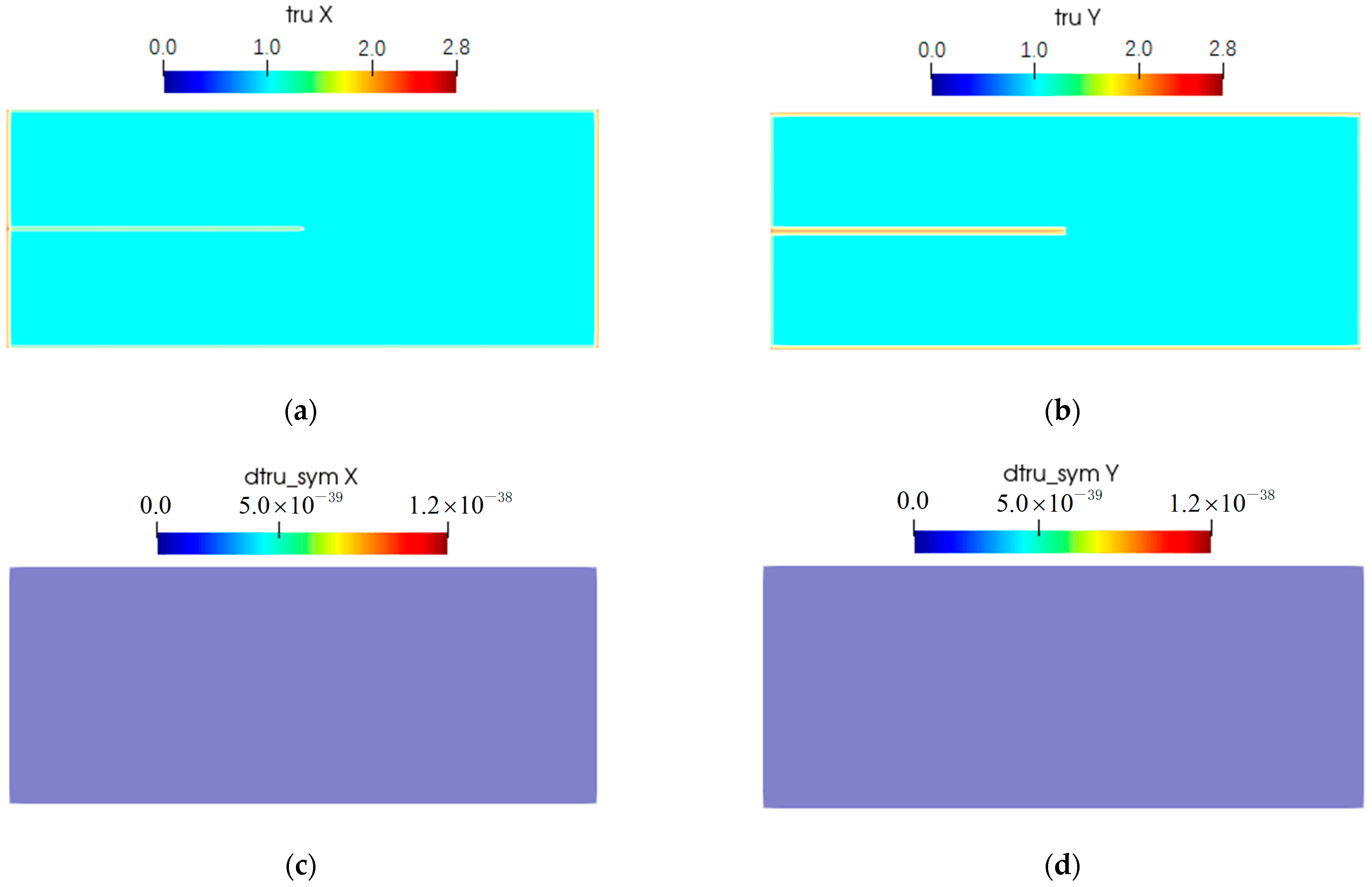
In order to demonstrate the influence of the third strategy (S3) on the calculation results of the surface-correction factors, Equation (28) defines the difference in surface-correction factors between symmetric material points.
d t r u = t r u ( i ) t r u ( i sym )
where d t r u is the difference vector of the correction factor, t r u ( i ) is the surface-correction factor of material point i, which is obtained at the initial stage of the simulation, and i sym is the symmetric material point of material point i. As shown in Figure 13, the surface-correction factors and the factor differences between symmetric material points from Case 1 are provided. Obviously, in Case 1, after computing the surface-correction factors, the numerical model still maintains good symmetry.
Similar results from Case 3 are displayed in Figure 14. The most significant discrepancy in the calculation results is observed in the difference in the surface-correction factors between symmetric material points along the x-direction, as illustrated in Figure 13c and Figure 14c. Considering the consistency of other conditions in Case 1 and Case 3, we conclude that whether the third strategy (S3) is considered determines the correctness or error of the results in this context. Clearly, the third strategy (S3) shown in Figure 2b also contributes to enhancing the accuracy of numerical calculations.
When real variables are represented using double-precision floating-point numbers, the dimensionless model ensures a wider range of load conditions for which calculation results maintain high accuracy. In this work, cases of the pre-notched plated shown in Figure 8 subjected to traction stresses of 24 MPa, 30 MPa, 40 MPa and 50 MPa were investigated. To facilitate comparisons with the existing literature, the material of the plate in these cases is set to Soda-lime glass, of which the material properties are given in Table 4. The crack propagation paths from the four cases are displayed in Figure 15. It should be noted that the calculations presented here are solely intended to demonstrate the effectiveness of the dimensionless model and precision-enhancing strategies in improving numerical accuracy, without addressing the convergence of the results.
The calculation results presented in Figure 15a exhibit high consistency with those reported in the literature [44], which further validates the correctness of the dimensionless PD model. The computational results under the four loading conditions illustrated in Figure 15 all exhibit high symmetry. Though the results under high level tensile stresses may not strictly satisfy the discrete parameter independence condition, the observed symmetry demonstrates that the dimensionless modelling and the numerical strategies proposed in this study effectively enhances the computational accuracy of bond-based PD models.

5. Conclusions

In this work, a dimensionless bond-based PD model was established and several numerical strategies were proposed to enhance numerical simulation accuracy of PD models. An elastic-wave propagation problem and a crack-branching problem were investigated to validate the correctness of the dimensionless PD model. To further validate the effectiveness of the numerical strategies and the dimensional normalization on enhancing numerical accuracy, several numerical cases about a symmetric problem, i.e., the pre-notched plate under traction stress, in different conditions were investigated. Based on the analysis of the results and discussions, the following conclusions can be drawn.
(1)
The dimensionless modelling of the bond-based PD model is correct. This modelling reduces the magnitude discrepancy between the micro-modulus and bond stretches, thereby suppressing the propagation of rounding errors in bond stretches.
(2)
The strategy of sorting neighborhood members by their distance to the central material point, combined with the strategy of calculating the surface-correction factors locally within the horizon, can significantly improve the accuracy of numerical results.
(3)
Utilizing the double-precision format for storing real variables, combined with the dimensionless bond-based PD model and the numerical processing strategies, the propagation of computational errors can be effectively suppressed.

Author Contributions

Conceptualization, C.H. and X.C.; software, C.H.; validation, C.H.; writing—original draft preparation, C.H.; writing—review and editing, X.C.; visualization, C.H. and X.C.; supervision, X.C.; funding acquisition, C.H. All authors have read and agreed to the published version of the manuscript.

Funding

This research was funded by National Natural Science Foundation of China, grant number 12202167 and Natural Science Foundation of Jiangsu Province, grant number BK20210872.

Data Availability Statement

The data presented in this study are available on request from the corresponding author.

Conflicts of Interest

The authors declare no conflicts of interest.

References

  1. Song, J.-H.; Wang, H.; Belytschko, T. A Comparative Study on Finite Element Methods for Dynamic Fracture. Comput. Mech. 2008, 42, 239–250. [Google Scholar] [CrossRef]
  2. Xie, G.; Li, J.; Li, H.; Wang, L.; Li, X.; Geng, H. Crack Growth Evaluation Based on the Extended Finite Element and Particle Filter Combined Method. Eng. Anal. Bound. Elem. 2024, 169, 106004. [Google Scholar] [CrossRef]
  3. Bui, H.H.; Fukagawa, R.; Sako, K.; Ohno, S. Lagrangian Meshfree Particles Method (SPH) for Large Deformation and Failure Flows of Geomaterial Using Elastic-Plastic Soil Constitutive Model. Int. J. Numer. Anal. Methods Geomech. 2008, 32, 1537–1570. [Google Scholar] [CrossRef]
  4. Fan, S.; Guilin, W.; Liang, Z.; Runqiu, W.; Tianci, C.; Xiaotian, O. Material Point Method for the Propagation of Multiple Branched Cracks Based on Classical Fracture Mechanics. Comput. Methods Appl. Mech. Eng. 2021, 386, 114116. [Google Scholar] [CrossRef]
  5. Zhao, Y.; Xin, T.; Tang, S.; Wang, H.; Fang, X.; Hou, H. Applications of Unified Phase-Field Methods to Designing Microstructures and Mechanical Properties of Alloys. MRS Bull. 2024, 49, 613–625. [Google Scholar] [CrossRef]
  6. Silling, S.A. Reformulation of Elasticity Theory for Discontinuities and Long-Range Forces. J. Mech. Phys. Solids 2000, 48, 175–209. [Google Scholar] [CrossRef]
  7. Silling, S.A.; Askari, E. A Meshfree Method Based on the Peridynamic Model of Solid Mechanics. Comput. Struct. 2005, 83, 1526–1535. [Google Scholar] [CrossRef]
  8. Wu, T.; Xue, T.; Wang, Y. Non-Fourier Thermoelastic Peridynamic Modelling of Cracked Thin Films Under Short-Pulse Laser Irradiation. Modelling 2025, 6, 68. [Google Scholar] [CrossRef]
  9. Le, Q.V.; Bobaru, F. Surface Corrections for Peridynamic Models in Elasticity and Fracture. Comput. Mech. 2018, 61, 499–518. [Google Scholar] [CrossRef]
  10. Jha, P.K.; Lipton, R. Numerical Convergence of Nonlinear Nonlocal Continuum Models to Local Elastodynamics. Int. J. Numer. Methods Eng. 2018, 114, 1389–1410. [Google Scholar] [CrossRef]
  11. Wu, X.; Chen, W. Error Estimates of the Finite Element Method for Interior Transmission Problems. J. Sci. Comput. 2013, 57, 331–348. [Google Scholar] [CrossRef]
  12. Lukacova-Medvid’ova, M.; Mizerova, H.; She, B.; Stebel, J. Error Analysis of Finite Element and Finite Volume Methods for Some Viscoelastic Fluids. J. Numer. Math. 2016, 24, 105–123. [Google Scholar] [CrossRef]
  13. Ohlberger, M.; Vovelle, J. Error Estimate for the Approximation of Nonlinear Conservation Laws on Bounded Domains by the Finite Volume Method. Math. Comput. 2006, 75, 113–150. [Google Scholar] [CrossRef]
  14. Palasis, A.; Liakopoulos, A.; Sofiadis, G. From Direct Numerical Simulations to Data-Driven Models: Insights into Mean Velocity Profiles and Turbulent Stresses in Channel Flows. Modelling 2025, 6, 18. [Google Scholar] [CrossRef]
  15. Violeau, D.; Fonty, T. Calculating the Smoothing Error in SPH. Comput. Fluids 2019, 191, 104240. [Google Scholar] [CrossRef]
  16. Steffen, M.; Kirby, R.M.; Berzins, M. Decoupling and Balancing of Space and Time Errors in the Material Point Method (MPM). Int. J. Numer. Methods Eng. 2010, 82, 1207–1243. [Google Scholar] [CrossRef]
  17. Ren, H.; Zhuang, X.; Rabczuk, T. Dual-Horizon Peridynamics: A Stable Solution to Varying Horizons. Comput. Methods Appl. Mech. Eng. 2017, 318, 762–782. [Google Scholar] [CrossRef]
  18. Moschou, S.P.; Hicks, E.; Parekh, R.Y.; Mathew, D.; Majumdar, S.; Vlahakis, N. Physics-Informed Neural Networks for Modelling Astrophysical Shocks. Mach. Learn. Technol. 2023, 4, 035032. [Google Scholar] [CrossRef]
  19. Luo, Y. Adaptive Nearest-Nodes Finite Element Method Guided by Gradient of Linear Strain Energy Density. Finite Elem. Anal. Des. 2009, 45, 925–933. [Google Scholar] [CrossRef]
  20. Gu, X.; Zhang, Q.; Xia, X. Voronoi-Based Peridynamics and Cracking Analysis with Adaptive Refinement. Int. J. Numer. Methods Eng. 2017, 112, 2087–2109. [Google Scholar] [CrossRef]
  21. Song, Y.; Yan, J.; Li, S.; Kang, Z. Peridynamic Modelling and Simulation of Ice Craters By Impact. Comput. Model. Eng. Sci. 2019, 121, 465–492. [Google Scholar] [CrossRef]
  22. Allahyari, M.; Yousefi, K.; Esfahanian, V.; Darzi, M. A Block-Interface Approach for High-Order Finite- Difference Simulations of Compressible Flows. J. Appl. Fluid Mech. 2021, 14, 345–359. [Google Scholar] [CrossRef]
  23. Daux, C.; Moës, N.; Dolbow, J.; Sukumar, N.; Belytschko, T. Arbitrary Branched and Intersecting Cracks with the Extended Finite Element Method. Int. J. Numer. Methods Eng. 2000, 48, 1741–1760. [Google Scholar] [CrossRef]
  24. Bautista, V.; Shahbazian, B.; Mirsayar, M. A Modified Mixed-Mode Timoshenko-Based Peridynamics Model Considering Shear Deformation. Int. J. Mech. Sci. 2025, 285, 109802. [Google Scholar] [CrossRef]
  25. Hou, Y.; Zhang, X. A Bond-Augmented Stabilized Method for Numerical Oscillations in Non-Ordinary State-Based Peridynamics. Eng. Fract. Mech. 2024, 307, 110276. [Google Scholar] [CrossRef]
  26. Wildman, R.A.; O’Grady, J.T.; Gazonas, G.A. A Hybrid Multiscale Finite Element/Peridynamics Method. Int. J. Fract. 2017, 207, 41–53. [Google Scholar] [CrossRef]
  27. Ha, Y.D.; Bobaru, F. Characteristics of Dynamic Brittle Fracture Captured with Peridynamics. Eng. Fract. Mech. 2011, 78, 1156–1168. [Google Scholar] [CrossRef]
  28. Liu, W.; Hong, J.-W. Discretized Peridynamics for Linear Elastic Solids. Comput. Mech. 2012, 50, 579–590. [Google Scholar] [CrossRef]
  29. Liu, Z.-G.; Du, S.-Y.; Yang, Y.; Ji, X.-H. A Fast Algorithm for Color Space Conversion and Rounding Error Analysis Based on Fixed-Point Digital Signal Processors. Comput. Electr. Eng. 2014, 40, 1405–1414. [Google Scholar] [CrossRef]
  30. Du, E.-B.; Zhou, X.-P. Non-Uniform Discretization Bond-Based Peridynamics with Constant Horizon and a Novel Volume Correction for the Cracking Behaviors. Comput. Struct. 2024, 300, 107408. [Google Scholar] [CrossRef]
  31. Shi, Y.; Niu, J.; Cai, M.; Xu, W. Dimensionless Study on Dynamics of Pressure Controlled Mechanical Ventilation System. J. Mech. Sci. Technol. 2015, 29, 431–439. [Google Scholar] [CrossRef]
  32. Huang, R.; Wu, H. A Modified Multiple-Relaxation-Time Lattice Boltzmann Model for Convection-Diffusion Equation. J. Comput. Phys. 2014, 274, 50–63. [Google Scholar] [CrossRef]
  33. Mandel, R.; Shooshtari, A.; Ohadi, M. A “2.5-D” Modelling Approach for Single-Phase Flow and Heat Transfer in Manifold Microchannels. Int. J. Heat Mass Transf. 2018, 126, 317–330. [Google Scholar] [CrossRef]
  34. Zhou, G.; Xie, Z.-W.; Xu, X.-H.; Li, Q. A New Model of Overall Heat Transfer Coefficient of Hot Wax Oil Pipeline Based on Dimensionless Experimental Analysis. Case Stud. Therm. Eng. 2020, 20, 100647. [Google Scholar] [CrossRef]
  35. Laporte-Azcue, M.; Acosta-Iborra, A.; Otanicar, T.P.; Santana, D. Real-Time Estimation of the Transient Thermomechanical Behaviour of Solar Central Receivers. Therm. Sci. Eng. Prog. 2023, 41, 101834. [Google Scholar] [CrossRef]
  36. Zhang, X.; Xu, X. A Moving Finite Element Method for Solving Two-Dimensional Coupled Burgers’ Equations at High Reynolds Numbers. Appl. Math. Lett. 2022, 133, 108271. [Google Scholar] [CrossRef]
  37. Protsenko, V.S.; Danilov, F.I. Application of Dimensional Analysis and Similarity Theory for Simulation of Electrode Kinetics Described by the Marcus-Hush-Chidsey Formalism. J. Electroanal. Chem. 2012, 669, 50–54. [Google Scholar] [CrossRef]
  38. Zhou, H.; Han, Y.; Zhang, Y.; Luo, W.; Liu, J.; Yu, R. Numerical and Experimental Research on Similarity Law of the Dynamic Responses of the Offshore Stiffened Plate Subjected to Low Velocity Impact Loading. Metals 2022, 12, 657. [Google Scholar] [CrossRef]
  39. IEEE Computer Society. IEEE Standard for Floating-Point Arithmetic 2019; The Institute of Electrical and Electronics Engineers: New York, NY, USA, 2019. [Google Scholar]
  40. Xie, K.; Lu, Q.; Jiang, H.; Wang, H. Accurate Sum and Dot Product with New Instruction for High-Precision Computing on ARMv8 Processor. Mathematics 2025, 13, 270. [Google Scholar] [CrossRef]
  41. Madenci, E.; Oterkus, E. Peridynamic Theory and Its Applications; Springer: New York, NY, USA, 2014; ISBN 9781461484653. [Google Scholar]
  42. Tong, Q.; Li, S. Multiscale Coupling of Molecular Dynamics and Peridynamics. J. Mech. Phys. Solids 2016, 95, 169–187. [Google Scholar] [CrossRef]
  43. Ha, Y.D.; Bobaru, F. Studies of Dynamic Crack Propagation and Crack Branching with Peridynamics. Int. J. Fract. 2010, 162, 229–244. [Google Scholar] [CrossRef]
  44. Bie, Y.H.; Liu, Z.M.; Yang, H.; Cui, X.Y. Abaqus Implementation of Dual Peridynamics for Brittle Fracture. Comput. Methods Appl. Mech. Eng. 2020, 372, 113398. [Google Scholar] [CrossRef]
Figure 1. Material point order in the horizon of a material point for a symmetric problem.
Modelling 06 00099 g001
Figure 2. Illustration of the X-displacement under a constant strain in X-direction. (a) Globally. (b) Locally. (In horizon).
Modelling 06 00099 g002
Figure 3. Illustration of a square plate with initial displacement.
Modelling 06 00099 g003
Figure 4. The initial displacement.
Modelling 06 00099 g004
Figure 5. History of the elastic potential energy.
Modelling 06 00099 g005
Figure 6. Displacement from dimensionless bond-based PD model. (a) 0 μs (b) 10 μs. (c) 20 μs (d) 30 μs. (e) 40 μs. (f) 50 μs. (g) 60 μs (h) Colorbar.
Modelling 06 00099 g006
Figure 7. Displacement from finite-element method. (a) 0 μs. (b) 10 μs. (c) 20 μs. (d) 30 μs. (e) 40 μs. (f) 50 μs. (g) 60 μs. (h) Colorbar.
Modelling 06 00099 g007
Figure 8. Traction of a pre-notched plate.
Modelling 06 00099 g008
Figure 9. Comparison of the crack path at 42.5 μs.
Modelling 06 00099 g009
Figure 10. Energy conversion. (a) Work and total energy. (b) Elastic potential and energy loss.
Modelling 06 00099 g010
Figure 11. Crack propagation paths from different models at 35 μs. (a) The dimensionless model. (b) The original model.
Modelling 06 00099 g011
Figure 12. Crack propagation paths from Case 3 at 35 μs.
Modelling 06 00099 g012
Figure 13. Surface-correction factors in Case 1. (a) Factor in x-direction. (b) Factor in y-direction. (c) Factor difference with symmetric point in x-direction. (d) Factor difference with symmetric point in y-direction.
Modelling 06 00099 g013
Figure 14. Surface-correction factors in Case 3. (a) Factor in x-direction. (b) Factor in y-direction. (c) Factor difference with symmetric point in x-direction. (d) Factor difference with symmetric point in y-direction.
Modelling 06 00099 g014
Figure 15. Crack paths in the pre-notched plate under different load levels. (a) σ = 24 MPa (t = 32.5 μs). (b) σ = 30 MPa (t = 32.5 μs). (c) σ = 40 MPa (t = 30.0 μs). (d) σ = 50 MPa (t = 25.0 μs).
Modelling 06 00099 g015
Table 1. Material properties of the square plate.
Density/(kg/m3)Young’s Modulus/(GPa)Poisson’s Ratio
2700.068.91/3
Table 2. Detailed parameters of the Duran 50 glass plate.
Young’s Modulus/GPaDensity/kg∙m−3Poisson’s RatioFracture Energy/JLength/mWidth/mCrack Length/m
6522350.22040.10.040.05
Table 3. Cases and strategies.
Case No.StrategiesModel
1Both S12 and S3Dimensionless PD
2Both S12 and S3Original PD
3Only S12Dimensionless PD
Table 4. Material properties of the Soda-lime glass.
Young’s Modulus/GPaDensity/kg∙m−3Poisson’s RatioFracture Energy/J
7224400.22135
Disclaimer/Publisher’s Note: The statements, opinions and data contained in all publications are solely those of the individual author(s) and contributor(s) and not of MDPI and/or the editor(s). MDPI and/or the editor(s) disclaim responsibility for any injury to people or property resulting from any ideas, methods, instructions or products referred to in the content.