Abstract
In three-dimensional (3D) logistics environments, finding optimal paths for unmanned aerial vehicles (UAVs) is challenging due to positioning inaccuracies that require ground-based corrections. These inaccuracies are exacerbated in harsh environments, leading to a significant risk of correction failure. This research proposes a multi-objective mixed integer programming model (MILP) that transforms dynamic uncertainties into binary constraints, utilizing a hierarchical sequencing strategy in the Gurobi optimizer to efficiently identify optimal paths. Our simulations indicate that achieving an 80% mission success probability necessitates an optimal path of 104,946 m with nine corrections. For a 100% success rate, the path length increases to 105,874 m, with corrections remaining constant. These results validate the model’s effectiveness in navigating environments with probabilistic constraints, highlighting its potential for addressing complex logistical challenges.
1. Introduction
Unmanned aerial vehicles (UAVs) can complete various tasks through preset routes, autonomous flight control systems, or remote wireless control. In the logistics industry, UAVs play an increasingly important role, and their application has become an area of great concern [1,2,3,4,5]. Compared with traditional logistics methods, drones can fly over ground traffic bottlenecks and obstacles to transport goods quickly and flexibly, improving transportation speed and efficiency [6]. UAVs can also be used for E-commerce retailers [7], postal services, and package delivery [8]. In disaster areas or areas where supplies are urgently needed, they can quickly deliver medical, food, and other urgently needed supplies, improving the effectiveness of emergency supplies [5,9,10,11]. Moreover, UAVs are expected to gradually replace traditional logistics transportation methods and become the mainstream of the logistics industry [12]. While the research on point-to-point path planning is crucial in the application of drone logistics and transportation [13]. This issue is concerned with identifying the most efficient path from a start point to a destination, avoiding obstacles, optimizing energy consumption, achieving the shortest route, and minimizing transit time [14].
Many methods and algorithms have been developed to address this complex challenge. For static obstacles, the Dijkstra algorithm determines the shortest path to the target point while considering the 2D and 3D models [15,16]. A voxel model is present to plan universal paths for drones in a known three-dimensional (3D) indoor environment with many static obstacles [17]. For some known and static threat environments on the sea, a hybrid differential evolution with quantum-behaved particle swarm optimization was successfully developed [18]. Several approaches to handle multiple constraints are addressed by mixed integer linear programming (MILP) formulations [19,20]. When the environment’s conditions are fully known and remain constant, determining a UAV’s route is considered static or global path planning [21]. Conversely, when the environment is entirely or partly unknown, local or dynamic path planning techniques are employed [22].
The exploration of dynamic path planning has recently attracted considerable attention from researchers and professionals. For instance, literature [14,23,24,25] present optimal UAV path planning methods based on MILP. The rapidly exploring random tree (RRT) algorithm is used to develop a real-time probabilistically robust path planner [26]. The hierarchical rapidly exploring random tree algorithm based on potential function lazy planning and low-cost optimization (HPO-RRT*) is proposed in dynamic environments with moving threats [27]. A Voronoi diagrams (VD) based algorithm is introduced for optimizing UAV path for maximizing the remaining energy in sensors after data transmission [28].
Beyond these classic methodologies, research in dynamic programming for UAV path planning has extended to the utilization of heuristic algorithms and meta-heuristic algorithms, such as the nearest-neighbor search algorithm [29], the multi-Strategy Fusion Differential Evolution algorithm (MSFDE) [30], the improved lazy theta* algorithm [31], the improved particle swarm optimization algorithm (PSO) [32], the adaptive path planning method PSO method (APP-PSO) [33], the dynamic group-based cooperative optimization (DGBCO) [34], hybrid simplified grey wolf optimizer and modified symbiotic organisms search method (HSGWO-MSOS) [35], and the improved Ant Colony Optimization algorithm (ACO) [36]. In addition, research on path planning based on sampling and machine learning has also achieved fruitful results, such as Sampling-based path planning [37], double deep-network (D3QN) [38], the attention-based pointer network (A-Ptr-Net) model [39], and deep reinforcement learning [40,41].
Practical UAV delivery also depends on launch/recovery platforms. Common modes include truck–drone cooperation (mobile launch) [42], rooftop/vertiport and micro-hub operations (fixed launch) [43], public transport-assisted delivery [44,45], and maritime/port platforms (barge/ship) [46,47]. These options can be integrated into our formulation by restricting admissible launch/landing nodes, adding basic capacity/turnaround limits, and synchronizing with platform schedules or kinematics. The current UAV logistics system relies on communication between ground base stations and drones [48]. In this study, we adopt a fixed-station structure: the UAV departs from A and must reach B; along the way a given finite set of ground-based stations (GBSs) provides vertical (VCS) or horizontal (HCS) corrections, with station locations/types known a priori; each mission serves a single user destination (B), while station scheduling/charging and parcel allocation beyond selecting B are treated exogenously; our optimization, therefore, focuses on selecting a sequence of GBSs and constructing the A–B path under GBS-provided environmental/communication information with probabilistic correction success. However, communication capabilities are easily affected by environmental factors [49]. Therefore, efficiently searching for robust and feasible paths for UAVs in uncertainty poses a challenging and intriguing research frontier [26]. In this paper, we study the optimal path problem of UAVs with the uncertainty of interference in communication between ground base stations and UAVs. We devised a multi-objective mixed linear integer programming model to address this issue and transform dynamic uncertainty into binary probability constraints. Leveraging the formidable computing capabilities of Gurobi Optimizer [50], we can obtain the global optimal solution, enabling efficient path planning in uncertain environments.
2. Problem Formulation
In complex environments, the issue of rapid trajectory planning is of significant importance. Notably, numerous constraints are encountered in the domain of low-cost UAVs used for logistics transportation. These include the lack of high-precision sensors, limited computational resources, restricted error correction capabilities, and reduced resistance to interference. These limitations result in the UAVs’ positioning systems’ inability to accurately self-locate, leading to potential mission failure should positioning errors accumulate beyond a critical threshold. Consequently, rectifying positioning errors during flight is imperative within the trajectory planning framework for intelligent aerial platforms. This research investigates the challenges of rapid trajectory planning for UAVs, specifically under the constraints imposed by system positioning accuracy.
Throughout the trajectory of a UAV, it is imperative to traverse waypoints positioned at varying altitudes and bearings, necessitating the provision of real-time positional data. The inaccuracies in positioning manifest as vertical and horizontal errors. With an assumption, these deviations are quantified and depicted in Figure 1, establishing a proportional relationship between the error magnitude, l, in meters, and the traversed aerial distance, L, in meters, articulated as follows:
where represents a proportionality constant. This mathematical representation encapsulates the relationship between flight distance and the resultant positioning error, both horizontally and vertically. Therefore, UAVs necessitate rectifying positional inaccuracies during flight, facilitated by Ground-Based Stations (GBS). Timely correction of vertical and horizontal positioning errors is crucial to ensure the UAV adheres to its predetermined flight path, which involves the iterative adjustment of errors via multiple GBSs.
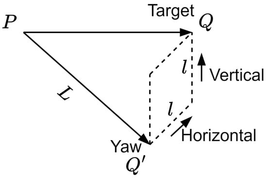
Figure 1.
Deviation diagram of a UAV.
The designated flight region for the UAV is depicted in Figure 2, commencing at point A and terminating at point B. The UAV undergoes corrections from various GBSs throughout the flight. As illustrated in Figure 2, the black triangle and blue triangle signify vertical and horizontal correction ground base stations (noted as VCS and HCS), respectively. The pink and red triangles represent VCSs and HCS with probabilistic constraints, respectively. In Figure 2, the contour represents the terrain elevation profile across the designated UAV flight region. The isoclines (contour lines) indicate equal altitude levels. Both the x-axis and y-axis represent spatial coordinates in meters, forming a 2D ground projection of the environment.
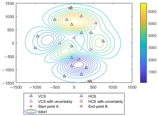
Figure 2.
The designated flight region for the (UAV).
This research addresses the challenge of swift trajectory planning for UAVs, considering the constraints posed by system positioning accuracy. The operational flight area for the UAV is depicted in Figure 2, with the starting point A and the destination B. The rules for GBS selection are as follows:
- Constr1.
- Both vertical and horizontal inaccuracies must remain beneath a threshold of meters upon arrival at destination B;
- Constr2.
- At the starting point A, both the vertical and horizontal errors of the UAV are 0;
- Constr3.
- Upon executing horizontal/vertical error correction at an HCS/VCS, the UAV’s horizontal/vertical error is reduced to zero, whereas its vertical/horizontal error remains unaffected;
- Constr4.
- Vertical error correction is permissible only if the UAV’s vertical error is below meters and its horizontal error does not exceed meters, as delineated in Figure 3a.
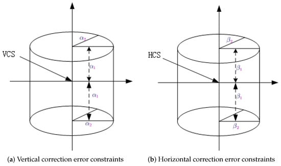 Figure 3. The UAV correction error constraints.
 - Constr5.
- Horizontal error correction is feasible when the UAV’s vertical error is under meters and its horizontal error is less than meters, as detailed in Figure 3b.
The environment of UAVs is subject to dynamic changes over time. Although corrections are predetermined before flight, achieving the ideal correction, defined as reducing a specific error to zero, is often impeded by uncontrollable factors such as weather conditions. As a result, when a UAV reaches a designated correction point, it may not be able to perform the intended error correction optimally. In this context, the probability that some GBSs can implement perfect correction is p.
- Constr6.
- By these GBSs, the corrected error is expressed aswhere represents the error before correction, and is a constant, with denoting a function that selects the smaller of two values.
Consequently, adherence to the planned trajectory entails a certain probability of mission failure.
This study must account for the energy constraints imposed by the UAV’s energy limitation, necessitating the optimization of the flight distance, minimization of the number of planned trajectories, and maximization of the probability of a successful mission. In the subsequent sections, we detail the optimization method and its application to trajectory optimization.
3. The MILP Model with Probability Constraints
A UAV’s trajectory is delineated by a sequence of GBSs , where denotes the indices of the GBSs involved, n represents the total number of available GBSs, and m signifies the number of GBSs incorporated within the planned path. Acknowledging that the UAV is constrained to follow a linear path between any two successive GBSs is imperative. The problem of UAV trajectory planning is inherently a non-linear optimization challenge characterized by multiple objectives and probability constraints. With a substantial quantity of GBSs available for inclusion in the trajectory planning process, selecting GBSs must adhere to predefined rules. The geographical coordinates and specific adjustment capabilities of these GBSs are known a priori, necessitating the selection of an optimal subset of GBSs to formulate the most efficient trajectory.
3.1. Decision Variable
Referring to Figure 4, the trajectory is also delineated as a sequence of segments , , …, , where each segment represents the Euclidean distance between GBS i and GBS j. In this context, the introduction of binary decision variables facilitates the modeling of the GBSs selection process. Specifically, when , it signifies the inclusion of the flight path segment in the UAV’s route. Conversely, denotes the exclusion of the segment from the flight plan. This binary framework enables a systematic approach to determining the optimal trajectory that adheres to predefined constraints and objectives.
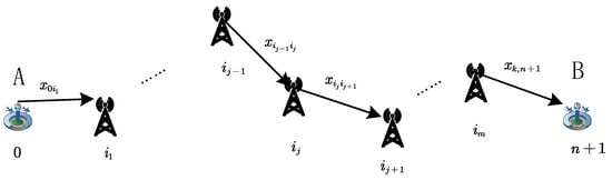
Figure 4.
The trajectory of an Unmanned Aerial Vehicle (UAV).
As delineated in Table 1, the element positioned at the intersection of the i-th row and j-th column, denoted as , serves as a decision variable that indicates the connectivity status between the i-th and j-th GBSs. That is

Table 1.
Define decision variables as a reachable table.
The following matrix captures the connections across GBSs, facilitating the optimization of the UAV’s flight trajectory.
It is readily observable that the diagonal elements of the matrix are uniformly set to zero. This reflects the principle that no GBS is connected to itself, excluding the possibility of self-loops in the flight trajectory optimization model. Then,
Since the starting point A and the destination B, it is imperative to assert the existence of GBSs connected with A and B, respectively. Therefore, the following expressions hold.
and
For a given flight mission, each GBS is selected no more than once. This constraint ensures that the sum of the entries in each row and column of the corresponding matrix does not exceed one, reflecting the principle that a UAV can enter and exit each GBS at most once. These conditions are formally expressed as follows:
In one flight mission, each base station was selected at most 1. It is further analyzed that the value of 1 bounds the maximum summation of each row and each column of this matrix since every GBS can be entered and departed by a UAV no more than once. These conditions are formulated as follows:
and
3.2. Error Constraints
3.2.1. The First GBS Selection
As depicted in Figure 5, two options are available for the first GBS to correct the error. We introduce classification variables for the correction types of the GBS as
where .
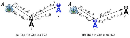
Figure 5.
The first and the second GBSs selection.
Therefore, according to the Constr4. and Constr5. as shown in Figure 3, the first selected GBS must satisfy
and
In Equations (10) and (11), the term represents the estimated total positioning error of the UAV at the time it reaches the i-th ground base station (GBS). Specifically,
- The denotes the Euclidean distance between the starting point A and the i-th GBS;
- The is a scalar coefficient that the error accumulation rate per unit distance;
- The product quantifies the magnitude of the UAV’s positioning error when requesting correction from GBS i.
These errors encompass both vertical and horizontal components. To ensure feasible error correction, constraints are established based on the type of correction available from the selected GBS:
- If , the GBS provides horizontal correction. The corresponding thresholds are and for vertical and horizontal errors, respectively.
These thresholds are defined in Constr4. and Constr5., and illustrated in Figure 3.
Constraints (10) and (11) are applicable when there is a connection between A and GBS i. In instances where A and the i-th GBS are not connected, the left-hand side of the inequalities defaults to 0. Therefore, the above constraints become
and
Since there is only one GBS connected to point A, combining with Equation (5), we integrate the constraints (12) and (13) as
and
Consequently, constraints (14) and (15) will function as constraints in the selection of the first GBS.
3.2.2. The Second GBS Constraints
As illustrated in Figure 5, two alternatives exist for the second GBS. Compared with the first GBS, the constraints at the second GBS are more stringent. Thus, by the rules Constr4. and Constr5. as depicted in Figure 3, the second GBS must fulfill
and
Reflecting the approach taken with the first GBS constraints, by integrating Equations (5) and (7), the constraints (16) and (17) are reformulated as
and
for .
3.2.3. The Other GBSs Selection
In the selection strategy for GBS, two categories of options emerge. The first scheme is that two adjacent GBSs belong to the same correction type. Conversely, the second one is that two adjacent GBSs are classified under differing correction types, as illustrated in Figure 6.
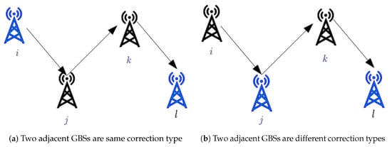
Figure 6.
The selection strategy for GBS.
Consider a scenario where four contiguous GBSs and l are identified along a trajectory as shown in Figure 6a. If GBS i and l are classified as the same type (either VCS or HCS), and GBS j and k differ in type from i and l, then the following constraint must be held for the GBS .
and
By integrating the constraints in (7) and (8), we can reformulate the previously stated constraints (20) and (21) as
and
for .
As shown in Figure 6b, when the GBS i and GBS k are of identical type, and the GBSs j and l differ from the former pair, then the constraints expressed in Equations (22) and (23) can also be satisfied for the GBS l. In this instance, it is pertinent to note that for the GBS l, it is only necessary to account for the cumulative errors associated with and . Consequently, the aforementioned constraints (22) and (23) can be simplified as follows:
and
for .
3.2.4. The Constraints of Destination B
As outlined in Section 2, it is imperative that both vertical and horizontal deviations remain below a threshold of meters upon arrival at the terminal point B. Figure 7 illustrates that the constraints are derived as follows:
and
Combining constraint (8), above constraints (26) and (27) can be expressed as
and
Thus, we derive the general constraint applicable to destination B as constraints (28) and (29).
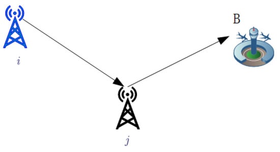
Figure 7.
The trajectory of endpoint.
3.3. Probability Constraints
Preliminaries and Notation
During a mission the environment may evolve and some corrections can fail (pink/red triangles in Figure 2). Each GBS succeeds in fully eliminating the accumulated error with probability ; if the attempt fails, the residual error is given by (2), which may jeopardise the mission. Trajectory planning must therefore account for the probability of mission success.
Let be the set of all feasible trajectories:
The m GBSs visited by x are
For a given potentially unreliable station , define
In other words, collects all trajectories that can tolerate exactly one correction failure—at GBS —while still completing the mission. Note that and, by construction, may be empty for some . To quantify mission success under uncertain corrections, we next formalize the station-level outcomes for each potentially unreliable GBS . Define the elementary random events as follows:
- : “the correction performed by GBS succeeds”; ;
- : “the correction performed by GBS fails”; ;
- : “the entire mission is completed successfully when the trajectory contains GBS ”.
is the probability of successful correction of GBS , while is the probability of failure correction. Denote the random event of successful correction at the GBS as , and the failure correction event is . Then,
Let the random event denote the success of a flight mission, whereas signifies the failure of the flight mission for the given GBS . Based on this definition, the conditional probability of an event can be expressed as
and
Consequently, in the presence of a GBS , the probability of success is
Extending to the m potentially unreliable stations visited along x, the overall mission-success probability , i.e., the probability that the UAV ultimately reaches its final waypoint B with all accumulated errors kept within allowable bounds, can be expressed as
Define binary variables ,
Thus,
Convert the above probability into a linear function
This probability Equation (39) is equivalent to the following equation:
where are the binary variables and satisfy
and
When , implying successful correction of GBS i, then equals 0; for , may be either 0 or 1.
As depicted in Figure 8, a UAV traverses i-th GBS to j-th GBS and subsequently from j-th GBS to k-th GBS. Assume that the i-th GBS is subject to probability constraints; a correction failure results in a residual error denoted by . To guarantee the successful execution of the flight mission, the error at the k-th must meet the following constraints:
and
where and . Therefore, according to the above definition of feasible solution set, can be expressed as
In reality, the set represents instances wherein GBS i effectively rectifies the error of the UAV. Under such circumstances, the accumulated error adheres to the established correction constraints. Conversely, failure in error correction results in the accumulated error breaching the error constraint threshold, leading to mission failure. Consequently, modifications to the aforementioned constraints (44) and (53) yield the following formulation:
and
where and . Thus, the set is represented as
Let denote the minimum acceptable mission-success probability prescribed by the operator, then the success probability constraint is
The feasible solutions are denoted by a set as
When , the set is given by
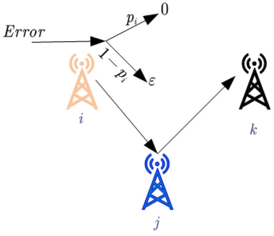
Figure 8.
Error changes at problem GBSs.
To summarize, Formulas (53) and (54) represent the constraints derived from the probability constraints we have established.
3.4. Objective Function
As described in Section 2, path planning for UAVs involves identifying an optimal path based on specified performance metrics. This study defines two critical performance indices: the path length and the number of GBSs involved.
The first objective,
aims to achieve the minimum possible flight distance. This objective is fundamental to optimizing the UAV’s energy consumption and operational time, extending its operational range and endurance.
The second objective, denoted as
focuses on minimizing the number of GBSs required during the UAV’s flight. GBSs are predefined locations where the UAV can adjust its flight path to ensure alignment with the mission’s objectives and constraints. Minimizing these points is crucial for enhancing flight efficiency and reducing operational complexity.
In summary, the model for purposes can be established as follows:
4. Experiment and Result
To validate the proposed model, an experiment was performed based on the dataset in [51], including GBSs’ locations (in meters), types, and identification of problem points. Table 2 lists the parameters of all constraints for this experiment.
Table 2.
Parameter setting in the optimization.
Formulating a multi-objective mixed-integer linear programming (MILP) problem presents a considerable challenge due to the extensive scale of constraints. In this study, we adopt a hierarchical multi-objective optimization strategy to solve the proposed mixed-integer linear programming model. Using Gurobi 10.0.1, we first minimize the number of correction points; keeping this optimal value fixed, we then optimize the total flight distance. The sequential MILP procedure—implemented via branch-and-bound and cutting-plane techniques—retains the finite-convergence and global-optimality guarantees of integer programming, ensuring that the second-level solution never degrades the primary objective and that the final lexicographic solution is mathematically certified [52,53].
When the probability of a successful flight mission is 80%, the set is represented by (53). Figure 9 demonstrates the optimal planned trajectory of the UAV with 80% success probability. The alteration in the hue of the triangle depicted in Figure 9 signifies the variance in altitude of the GBS.
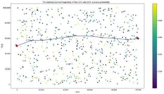
Figure 9.
The optimal planned trajectory of the UAV with 80% success probability.
The entire distance of the trajectory is 104,946 meters, necessitating the incorporation of nine GBSs. As delineated in Figure 10, the GBSs 503 and 91 are VCSs with probability constraints, and 294 is an HCS with probability constraints. Additionally, GBSs 33, 403, and 501 are VCSs, whereas GBSs 233, 315, and 594 are HCSs. The process of correction, which alternates between horizontal and vertical points, is conducted throughout the flight. The errors in the Figure 10a show that the corrections of the three GBSs at 503, 294, and 91 are all successful.
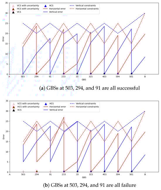
Figure 10.
The errors at the GBSs and target B along the optimal planned trajectory of the UAV with 80% success probability.
The red dotted line represents the horizontal error limit of the corresponding type of GBS, and the red solid line represents the horizontal cumulative error of the UAV. Figure 10a shows that during the flight of the UAV, the horizontal cumulative error does not exceed the horizontal error limit. The blue dotted line represents the vertical error limit of the corresponding GBS, and the blue solid line represents the vertical cumulative error change in the UAV. Figure 10a shows that the vertical cumulative error did not exceed the vertical error limit during the UAV flight.
Conversely, the errors in Figure 10b show that the corrections of the three GBSs at 503, 294, and 91 are all failures. Figure 10b illustrates a scenario where the correction attempt at GBS 294 is unsuccessful, leading to a breach of constraint requirements at GBS 233 and consequently failing the flight mission. Failures in correction attempts at points 503 and 294 did not impinge upon the execution of the flight mission. Given that the probability of a successful correction for point 294 stands at 0.8, the overall probability of success for all designated tasks is estimated at 80%.
Figure 11 delineates the optimal flight trajectory, achieving a success probability of 100%. The trajectory is a total of 105,873 meters and traverses nine GBSs, with horizontal and vertical corrections implemented alternately. Figure 12 identifies GBSs 503 and 506 as VCSs subject to probability constraints and GBS 69 as an HCS with probability constraints. Moreover, GBS 371, 194, and 286 are HCSs, while points 183, 450, and 368 are VCSs. The analysis presented in Figure 12a,b confirms that the cumulative error remains within the error correction parameters, ensuring the successful completion of the flight mission. Consequently, this trajectory secures a mission success probability of 100%. The errors in Figure 12b show that the corrections of the three GBSs at 503, 69, and 506 all failed, and the flight missions were successful. These two experiments show that our model can solve probabilistic constraints and quickly obtain optimal solutions.
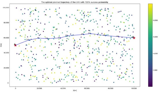
Figure 11.
The optimal planned trajectory of the UAV with 100% success probability.
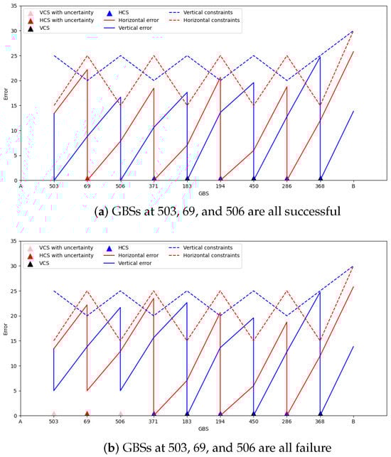
Figure 12.
The errors at the GBSs and destination B in the planed path of the UAV with 100% success probability.
To examine the robustness and applicability of the presented model, a second numerical example (Case 2) was used for a computational experiment, which is shown alongside that from Case 1 in Table 3. This additional case applies a set of stricter parameters, requiring smaller error bounds (, ) and higher precision for the correction angle (), to simulate an environment with more urgent operational conditions where safety requirements are tighter.
Table 3.
Two-case comparison of routing outcomes across the minimum acceptable mission success levels s.
As can be seen from the results, reducing s all along causes a consistent decrease in either total trajectory length or required correction points (CPS). In Case 1, with the success probability varying from 100% to 64%, we find that when it changes gradually, CPS has no variant transformation while the trajectory length is shortened slightly from 105,873 to 104,065 m. On the other hand, more restrictive assumptions in Case 2 impose a remarkable decrease on CPS (from 21 to 16) and trajectory distance from 165,615 to 128,740 m, when the demanded probability diminishes from a deterministically imposed value of 100% to 64%. These results emphasize that the reduction in reliability demands in highly restricted operational scenarios leads to a significant bias.
Considering this scenario, the proposed MILP-based optimization model is able to provide close-to-optimal solutions for different operational conditions and reliability requirements. This verification demonstrates the practical applicability of our method, which is helpful for decision-makers to balance between mission reliability and operational efficiency in real-world drone logistics.
5. Conclusions
In this paper, set within a three-dimensional (3D) context and accounting for uncertainties related to UAV positioning errors and ground base station corrections, a multi-objective mixed integer linear programming (MILP) model was developed, incorporating probability constraints. Utilizing the hierarchical sequential method of the Gurobi optimizer, the model facilitates a more adaptable decision-making process by adjusting the optimization sequence according to the priorities of different targets. Integrating this model with the Gurobi optimizer allows for rapid resolution and acquisition of the global optimum and showcases an efficient approach to tackling complex challenges. This methodology proves particularly effective in logistics transportation path planning within disaster-stricken or war-torn regions, confronting multiple uncertainties. It significantly enhances the reliability and practical applicability of path-planning strategies.
This study addresses shortest-path planning for a single UAV with a fixed set of ground-based stations (GBSs). Parcel–station assignment and station operations are treated as given; correction success is modeled as independent and time-invariant; planning is offline and energy, safety, and weather effects are simplified. In the future, we will focus on two directions: (i) endogenizing the infrastructure by jointly optimizing station selection, capacity/turnaround, and parcel–station assignment together with routing and (ii) developing data-driven, risk-aware, online methods that learn spatio-temporal (and correlated) reliability from telemetry and weather data to support chance constraints and real-time re-planning under updated GBS/environmental information.
Author Contributions
Conceptualization, Z.C. and S.W.; methodology, Z.C. and X.Z.; software, S.W.; validation, Z.C., S.W. and K.C.; formal analysis, Z.C.; investigation, Z.C.; resources, Z.C.; writing—original draft preparation, Z.C.; writing—review and editing, K.C.; visualization, S.W.; supervision, K.C. All authors have read and agreed to the published version of the manuscript.
Funding
This research and APC were supported by the Foundation of the Key Laboratory of National Defense Science and Technology granted number JZX7Y202301SY000601.
Institutional Review Board Statement
Not applicable.
Informed Consent Statement
Not applicable.
Data Availability Statement
https://github.com/Chenzx1259/drone/blob/main/droneuav.xlsx (accessed on 11 August 2025).
Acknowledgments
During the preparation of this study, the authors used [chatgpt, 3o] for the purposes of translation. The authors have reviewed and edited the output and take full responsibility for the content of this publication.
Conflicts of Interest
The authors declare no conflicts of interest.
References
- Moshref, J.M.; Winkenbach, M. Applications and Research avenues for drone-based models in logistics: A classification and review. Expert Syst. Appl. 2021, 177, 114854. [Google Scholar] [CrossRef]
- Kamat, A.; Shanker, S.; Barve, A.; Muduli, K.; Mangla, S.K.; Luthra, S. Uncovering interrelationships between barriers to unmanned aerial vehicles in humanitarian logistics. Oper. Manag. Res. 2022, 15, 1134–1160. [Google Scholar] [CrossRef]
- Bansal, S.; Goel, R.; Maini, R. Ground vehicle and UAV collaborative routing and scheduling for humanitarian logistics using random walk based ant colony optimization. Sci. Iran. 2022, 29, 632–644. [Google Scholar]
- Jiang, H.; Wu, T.; Ren, X.; Gou, L. Optimisation of Multi-Type Logistics UAV Scheduling under High Demand. Promet-Traffic Transp. 2024, 36, 115–131. [Google Scholar] [CrossRef]
- Law, C.T.; Moenig, C.; Jeilani, H.; Jeilani, M.; Young, T. Transforming healthcare logistics and evaluating current use cases of UAVs (drones) as a method of transportation in healthcare to generate recommendations for the NHS to use drone technology at scale: A narrative review. BMJ Innov. 2023, 9, bmjinnov-2021. [Google Scholar] [CrossRef]
- Thiels, C.A.; Aho, J.M.; Zietlow, S.P.; Jenkins, D.H. Use of unmanned aerial vehicles for medical product transport. Air Med. J. 2015, 34, 104–108. [Google Scholar] [CrossRef]
- Straubinger, A.; de Groot, H.L.; Verhoef, E.T. E-commerce, delivery drones and their impact on cities. Transp. Res. Part A Policy Pract. 2023, 178, 103841. [Google Scholar] [CrossRef]
- Buko, J.; Bulsa, M.; Makowski, A. Spatial premises and key conditions for the use of UAVs for delivery of items on the example of the polish courier and postal services market. Energies 2022, 15, 1403. [Google Scholar] [CrossRef]
- Merei, A.; Mcheick, H.; Ghaddar, A. Survey on Path Planning for UAVs in Healthcare Missions. J. Med. Syst. 2023, 47, 79. [Google Scholar] [CrossRef]
- Wen, T.; Zhang, Z.; Wong, K.K. Multi-objective algorithm for blood supply via unmanned aerial vehicles to the wounded in an emergency situation. PLoS ONE 2016, 11, e0155176. [Google Scholar] [CrossRef]
- Gao, W.; Luo, J.; Zhang, W.; Yuan, W.; Liao, Z. Commanding cooperative ugv-uav with nested vehicle routing for emergency resource delivery. IEEE Access 2020, 8, 215691–215704. [Google Scholar] [CrossRef]
- Huang, S. The technical principle and application case analysis of logistics UAV. Highlights Sci. Eng. Technol. 2023, 72, 474–479. [Google Scholar] [CrossRef]
- Lu, Y.; Xue, Z.; Xia, G.S.; Zhang, L. A survey on vision-based UAV navigation. Geo-Spat. Inf. Sci. 2018, 21, 21–32. [Google Scholar] [CrossRef]
- Qadir, Z.; Ullah, F.; Munawar, H.S.; Al-Turjman, F. Addressing disasters in smart cities through UAVs path planning and 5G communications: A systematic review. Comput. Commun. 2021, 168, 114–135. [Google Scholar] [CrossRef]
- Dijkstra, E.W. A note on two problems in connexion with graphs. Numer. Math. 1959, 1, 269–271. pp. 287–290. [Google Scholar] [CrossRef]
- Dhulkefl, E.; Durdu, A.; Terzioğlu, H. Dijkstra algorithm using UAV path planning. Konya J. Eng. Sci. 2020, 8, 92–105. [Google Scholar] [CrossRef]
- Li, F.; Zlatanova, S.; Koopman, M.; Bai, X. and Diakité, A. Universal path planning for an indoor drone. Autom. Constr. 2018, 95, 275–283. [Google Scholar] [CrossRef]
- Fu, Y.; Ding, M.; Zhou, C.; Hu, H. Route planning for unmanned aerial vehicle (UAV) on the sea using hybrid differential evolution and quantum-behaved particle swarm optimization. IEEE Trans. Syst. Man, Cybern. Syst. 2013, 43, 1451–1465. [Google Scholar] [CrossRef]
- Song, B.D.; Kim, J.; Morrison, J.R. Rolling horizon path planning of an autonomous system of UAVs for persistent cooperative service: MILP formulation and efficient heuristics. J. Intell. Robot. Syst. 2016, 84, 241–258. [Google Scholar] [CrossRef]
- Zuo, Y.; Tharmarasa, R.; Jassemi-Zargani, R.; Kashyap, N.; Thiyagalingam, J.; Kirubarajan, T.T. MILP formulation for aircraft path planning in persistent surveillance. IEEE Trans. Aerosp. Electron. Syst. 2020, 56, 3796–3811. [Google Scholar] [CrossRef]
- Babel, L. Coordinated target assignment and UAV path planning with timing constraints. J. Intell. Robot. Syst. 2019, 94, 857–869. [Google Scholar] [CrossRef]
- Chen, X.; Zhao, M.; Yin, L. Dynamic path planning of the UAV avoiding static and moving obstacles. J. Intell. Robot. Syst. 2020, 99, 909–931. [Google Scholar] [CrossRef]
- Radmanesh, M.; Kumar, M.; Nemati, A.; Sarim, M. Dynamic optimal UAV trajectory planning in the national airspace system via mixed integer linear programming. Proc. Inst. Mech. Eng. Part G J. Aerosp. Eng. 2016, 230, 1668–1682. [Google Scholar] [CrossRef]
- Liao, Y.; Friderikos, V. Energy and age pareto optimal trajectories in uav-assisted wireless data collection. IEEE Trans. Veh. Technol. 2022, 71, 9101–9106. [Google Scholar] [CrossRef]
- Qiu, R.; Liang, Y. A Novel Approach for Two-Stage UAV Path Planning in Pipeline Network Inspection. Int. Pipeline Conf. 2020, 84461, V003T04A011. [Google Scholar]
- Kothari, M.; Postlethwaite, I. A probabilistically robust path planning algorithm for UAVs using rapidly-exploring random trees. J. Intell. Robot. Syst. 2013, 71, 231–253. [Google Scholar] [CrossRef]
- Guo, Y.; Liu, X.; Jia, Q.; Liu, X.; Zhang, W. HPO-RRT*: A sampling-based algorithm for UAV real-time path planning in a dynamic environment. Complex Intell. Syst. 2023, 9, 7133–7153. [Google Scholar] [CrossRef]
- Baek, J.; Han, S.I.; Han, Y. Energy-efficient UAV routing for wireless sensor networks. IEEE Trans. Veh. Technol. 2019, 69, 1741–1750. [Google Scholar] [CrossRef]
- Shen, K.; Shivgan, R.; Medina, J.; Dong, Z.; Rojas-Cessa, R. Multidepot drone path planning with collision avoidance. IEEE Internet Things J. 2022, 9, 16297–16307. [Google Scholar] [CrossRef]
- Chai, X.; Zheng, Z.; Xiao, J.; Yan, L.; Qu, B.; Wen, P.; Wang, H.; Zhou, Y.; Sun, H. Multi-strategy fusion differential evolution algorithm for UAV path planning in complex environment. Aerosp. Sci. Technol. 2022, 121, 107287. [Google Scholar] [CrossRef]
- Yuan, M.S.; Chen, M. Improved lazy theta* algorithm based on octree map for path planning of UAV. Def. Technol. 2023, 23, 8–18. [Google Scholar] [CrossRef]
- Yu, Z.; Si, Z.; Li, X.; Wang, D.; Song, H. A novel hybrid particle swarm optimization algorithm for path planning of UAVs. IEEE Internet Things J. 2022, 9, 22547–22558. [Google Scholar] [CrossRef]
- Ma, Z.; Chen, J. Adaptive path planning method for UAVs in complex environments. Int. J. Appl. Earth Obs. Geoinf. 2022, 115, 103133. [Google Scholar] [CrossRef]
- Qadir, Z.; Zafar, M.H.; Moosavi, S.K.R.; Le, K.N.; Mahmud, M.P. Autonomous UAV path-planning optimization using metaheuristic approach for predisaster assessment. IEEE Internet Things J. 2021, 9, 12505–12514. [Google Scholar] [CrossRef]
- Qu, C.; Gai, W.; Zhang, J. and Zhong, M. A novel hybrid grey wolf optimizer algorithm for unmanned aerial vehicle (UAV) path planning. Knowl.-Based Syst. 2020, 194, 105530. [Google Scholar] [CrossRef]
- Li, T.; Peng, H.; Zhang, X.J. An UAV path planning method in mountainous area based on an improved ant colony algorithm. J. Transp. Syst. Eng. Inf. Technol. 2019, 19, 158. [Google Scholar]
- Lin, Y.; Saripalli, S. Sampling-based path planning for UAV collision avoidance. IEEE Trans. Intell. Transp. Syst. 2017, 18, 3179–3192. [Google Scholar] [CrossRef]
- Wang, X.; Gursoy, M.C.; Erpek, T.; Sagduyu, Y.E. Learning-based UAV path planning for data collection with integrated collision avoidance. IEEE Internet Things J. 2022, 9, 16663–16676. [Google Scholar] [CrossRef]
- Kong, F.; Li, J.; Jiang, B.; Wang, H.; Song, H. Trajectory optimization for drone logistics delivery via attention-based pointer network. IEEE Trans. Intell. Transp. Syst. 2022, 24, 4519–4531. [Google Scholar] [CrossRef]
- Li, B.; Wu, Y. Path planning for UAV ground target tracking via deep reinforcement learning. IEEE Access 2020, 8, 29064–29074. [Google Scholar] [CrossRef]
- Maw, A.A.; Tyan, M.; Nguyen, T.A.; Lee, J.W. iADA*-RL: Anytime graph-based path planning with deep reinforcement learning for an autonomous UAV. Appl. Sci. 2021, 11, 3948. [Google Scholar] [CrossRef]
- Murray, C.C.; Chu, A.G. The Flying Sidekick Traveling Salesman Problem: Optimization of Drone-Assisted Parcel Delivery. Transp. Res. Part C 2015, 54, 86–109. [Google Scholar] [CrossRef]
- Federal Aviation Administration (FAA). Engineering Brief No. 105A: Vertiport Design. FAA Eng. Brief 2024. Available online: https://www.faa.gov/airports/engineering/engineering_briefs/eb_105a_vertiports (accessed on 11 August 2025).
- Choudhury, S.; Solovey, K.; Kochenderfer, M.J.; Pavone, M. Efficient Large-Scale Multi-Drone Delivery Using Transit Networks. J. Artif. Intell. Res. 2021, 70, 757–788. [Google Scholar] [CrossRef]
- Liao, X.; Chen, Y. Drone Routing Problem Model for Last-Mile Delivery Using the Public Transportation System. PLoS ONE 2022, 17, e0266205. [Google Scholar]
- Yang, Y.; Hao, X.; Wang, S. The Drone Scheduling Problem in Shore-to-Ship Delivery: A Time Discretization-Based Model with an Exact Solving Approach. SSRN Work. Pap. 2024, 191, 103117. [Google Scholar] [CrossRef]
- Li, X.; Zhang, H. Cooperative Path Planning Optimization for Ship–Drone Delivery in Maritime Supply Operations. Complex Intell. Syst. 2025; in press. Available online: https://link.springer.com/article/10.1007/s40747-025-01837-5 (accessed on 11 August 2025).
- Xiao, Z.; Dong, H.; Bai, L.; Wu, D.O.; Xia, X.G. Unmanned aerial vehicle base station (uav-bs) deployment with millimeter-wave beamforming. IEEE Internet Things J. 2020, 7, 1336–1349. [Google Scholar] [CrossRef]
- Grotli, E.I.; Johansen, T.A. Path Planning for UAVs Under Communication Constraints Using SPLAT! and MILP. J. Intell. Robot. Syst. 2011, 65, 265–282. [Google Scholar] [CrossRef]
- Gurobi Optimization. Gurobi 10.0.1: Every Solution, Globally Optimized. 2023. Available online: https://www.gurobi.com (accessed on 11 August 2025).
- Drones Data. Available online: https://github.com/Chenzx1259/drone/blob/main/droneuav.xlsx (accessed on 11 August 2025).
- Wolsey, L.A. Integer Programming; Wiley–Interscience: Hoboken, NJ, USA, 1999. [Google Scholar]
- Nemhauser, G.L.; Wolsey, L.A. Integer and Combinatorial Optimization; John Wiley & Sons: Hoboken, NJ, USA, 1988. [Google Scholar]
Disclaimer/Publisher’s Note: The statements, opinions and data contained in all publications are solely those of the individual author(s) and contributor(s) and not of MDPI and/or the editor(s). MDPI and/or the editor(s) disclaim responsibility for any injury to people or property resulting from any ideas, methods, instructions or products referred to in the content. |
© 2025 by the authors. Licensee MDPI, Basel, Switzerland. This article is an open access article distributed under the terms and conditions of the Creative Commons Attribution (CC BY) license (https://creativecommons.org/licenses/by/4.0/).