A Conservative Four-Dimensional Hyperchaotic Model with a Center Manifold and Infinitely Many Equilibria

Abstract

This paper presents a novel four-dimensional autonomous conservative model characterized by an infinite set of equilibrium points and an unusual algebraic structure in which all eigenvalues of the Jacobian matrix are zero. The linearization of the proposed model implies that classical stability analysis is inadequate, as only the center manifolds are obtained. Consequently, the stability of the system is investigated through both analytical and numerical methods using Lyapunov functions and numerical simulations. The proposed model exhibits rich dynamics, including hyperchaotic behavior, which is characterized using the Lyapunov exponents, bifurcation diagrams, sensitivity analysis, attractor projections, and Poincaré map. Moreover, in this paper, we explore the model with fractional-order derivatives, demonstrating that the fractional dynamics fundamentally change the geometrical structure of the attractors and significantly change the system stability. The Grünwald–Letnikov formulation is used for modeling, while numerical integration is performed using the Caputo operator to capture the memory effects inherent in fractional models. Finally, an analog electronic circuit realization is provided to experimentally validate the theoretical and numerical findings.

1. Introduction

The foundations of chaos theory trace back to the early 20th century, when Henri Poincaré first observed that nonlinear dynamical systems can exhibit highly unpredictable behavior. During a study of the three-body problem, Poincaré discovered that small variations in initial conditions could lead to different trajectories, challenging the classical notion of determinism. Decades later, in 1963, Edward Lorenz formalized the concept of chaos by introducing a simple nonlinear model of atmospheric convection that demonstrated extreme sensitivity to initial conditions [1]. Since then, the analysis of chaotic systems has become a central theme in nonlinear dynamics, attracting extensive attention.

In 1970, Otto Rössler demonstrated that chaotic systems can exhibit higher levels of complexity when two or more positive Lyapunov exponents are present, a phenomenon later termed hyperchaos [2]. Chaotic and hyperchaotic systems are generally classified into two main categories: self-excited attractors and hidden attractors. Self-excited attractors are those whose basins of attraction intersect with the neighborhoods of unstable equilibrium points, making them detectable via standard computational procedures. In contrast, hidden attractors have basins that are disconnected from any equilibria, making their investigations more challenging [3,4,5,6].

Recent studies have explored four-dimensional chaotic and hyperchaotic systems with intricate dynamical behavior and non-polynomial nonlinearities, revealing complex bifurcation structures and multi-scroll attractors [7,8].

In the analysis of dynamical systems, equilibrium points play a fundamental role in understanding long-term behavior, such as stability, periodicity, or the onset of chaos. In particular, hyperbolic equilibria, where the Jacobian has no eigenvalues with zero real parts, often facilitate the application of linearization techniques. Numerous researchers have investigated chaotic systems that exhibit a variety of equilibrium structures, including systems with single, multiple, or even infinite equilibria. For more details, the reader is referred to [9,10].

Chaos and hyperchaos are ubiquitous phenomena in various scientific disciplines, including physics, mathematics, biology, and chemistry [11]. These complex behaviors have attracted considerable attention due to their fundamental role in the study of nonlinear dynamical systems [12,13,14,15].

The construction of new chaotic systems with special structural characteristics, such as algebraic properties, has become an active area of research. Notable examples include systems without equilibria [16], systems with stable equilibria [17], and systems whose equilibrium points lie along segmented lines [18,19].

Chaotic and hyperchaotic systems are also broadly categorized into dissipative and conservative classes. In dissipative systems, quantities such as energy are continuously lost, typically through friction or diffusion, ultimately leading to lower-dimension attractors [20]. In contrast, conservative hyperchaotic systems preserve total energy or other invariants over time. Despite their chaotic dynamics, the trajectories in such systems remain confined to bounded regions of phase space while maintaining constant energy levels. Recent studies have reported several examples of conservative chaotic systems with intricate dynamical behavior [21,22,23,24].

However, the local stability near equilibrium points offers a fascinating geometric perspective that underpins our understanding of the complex dynamics inherent in hyperchaotic systems. It highlights how seemingly simple mathematical structures can lead to intricate and unpredictable behavior. Although many hyperchaotic systems possess isolated equilibrium points, often located at the origin, others exhibit more exotic configurations, such as lines, curves, quadric surfaces, or even spherical manifolds of equilibria.

The stability of such systems is typically assessed through the eigenvalues of the associated Jacobian matrix. However, systems in which all eigenvalues are zero remain exceedingly rare in the literature, particularly in three- and four-dimensional cases. Analyzing the stability of these degenerate systems presents substantial mathematical challenges, as linearization fails to provide conclusive information.

To provide context and highlight the distinctiveness of the proposed system,

Table 1. Comparison of related identical chaotic and hyperchaotic systems.

Refs	Dim.	No. Systems	Equilibrium Type	Nonlin. Terms-Type
[25]	all 3D	9	all unstable	3-all quadratic
[26]	4D	1	unstable	5-cube
[27]	3D	1	unstable	7- trigonometric
[28]	3D	1	unstable	3-quadratic
This work	4D	1	stable	5- trigonometric

summarizes several known hyperchaotic systems with diverse equilibrium structures and stability characteristics.

Due to their rich and intricate dynamics, fractional-order autonomous systems have gained increasing attention in applications such as secure communication and advanced encryption technologies. For example, Rahman et al. [29] demonstrated that a specific four-dimensional fractional-order hyperchaotic system is particularly well suited for high-security communication schemes due to its sensitivity and complexity.

Fractional-order systems have gained considerable attention in recent years due to their ability to capture more accurately the memory and hereditary properties inherent in many physical and biological systems. In particular, they offer a richer dynamical framework than their integer-order counterparts, enabling more nuanced modeling of complex behaviors such as chaos, hyperchaos, and multistability. As highlighted in [26], the dynamics of conservative four-dimensional hyperchaotic systems under both integer and fractional derivatives were investigated, demonstrating how fractional calculus can significantly alter system behavior and stability characteristics. Fractional-order systems are typically categorized into two primary classes: commensurate systems, where all differential orders are equal, and incommensurate systems, where the orders vary among the equations, as elaborated in [30]. Moreover, the use of fractional derivatives has become a foundational approach in the study of chaotic systems, especially within the framework of memristive neural networks [31].

Further developments include the design of multi-wing chaotic attractors based on fractional-order extensions of the Li, Lü, and Chen systems [32], and methods for computing Lyapunov exponents in fractional-order chaotic systems [33]. The fractional-order modeling framework has also been used in various contexts, such as predator–prey population dynamics [34] and epidemiological modeling of Ebola virus spread [35], demonstrating the versatility and applicability of fractional calculus in modeling complex real-world phenomena.

Understanding and designing hyperchaotic systems with unconventional equilibrium structures and fractional dynamics presents several compelling research challenges. This study is driven by the following main considerations:

• Most existing hyperchaotic systems rely on isolated hyperbolic equilibria; however, systems with infinitely many equilibrium points, particularly with zero eigenvalues, are rarely studied and analytically challenging due to the failure of classical linearization methods.
• Conservative hyperchaotic systems are far less common than their dissipative ones, despite their theoretical importance in energy-preserving dynamics. This work introduces a novel system that combines conservative behavior, infinite equilibria, and center manifold.
• The study of fractional-order dynamical systems has gained momentum for its ability to capture memory effects and enhance system complexity. Extending conservative hyperchaotic systems to the fractional domain introduces new theoretical challenges and richer dynamical behavior.

In this paper, a new four-dimensional autonomous conservative system with a center manifold is proposed. The organization of this paper is as follows: in Section 2, the proposed four-dimensional differential systems are introduced. Section 3 introduces the analysis of the proposed stability system. In the next section, the complexity of the proposed system is investigated by computing the Lyapunov exponents, bifurcation diagram, Poincaré cross map, and the Kolmogorov–Sinai entropy. In Section 5, the fractional-order system described by Grunwald–Letnikov is displayed, utilizing the Lyapunov exponents of the fractional-order system, describing the type of chaos, and presenting phase portraits of different orders. Finally, in Section 6, the hardware implementation is discussed.

2. Proposed Model

Using five nonlinear terms including the sin function, we present the following system:

$$\left\{\begin{array}{cc}\dot{x}\hfill & =y,\hfill \\ \dot{y}\hfill & =-x^3-y{z}^3,\hfill \\ \dot{z}\hfill & =\alpha y^2+sin\left(w\right),\hfill \\ \dot{w}\hfill & =z^3,\hfill \end{array}\right.$$

(1)

where $\alpha >0$ is the system parameter. The parameter configuration of $\alpha =1.3$ to generate a strange attractor.

3. Stability Analysis

Solving algebraic equations: $\dot{x}=\dot{y}=\dot{z}=\dot{w}=0,$ system (1) has infinitely many equilibria ${\mathbf{E}}_{\mathbf{IM}}=(0,0,0,n\pi )$, where $n\in \mathbb{Z}.$ The Jacobian matrix J evaluated at any equilibrium ${\mathbf{E}}_{\mathbf{IM}}=(0,0,0,n\pi )$ is as follows:

$$J\left({\mathbf{E}}_{\mathbf{IM}}\right)=\left[\begin{array}{cccc}0& 1& 0& 0\\ 0& 0& 0& 0\\ 0& 0& 0& {(-1)}^n\\ 0& 0& 0& 0\end{array}\right].$$

(2)

The characteristic polynomial of the above matrix is given by $Pol(J{\mathbf{E}}_{\mathbf{IM}},\lambda )={\lambda }^4$, indicating that all eigenvalues are zero. This implies that system (1) is included in the zero manifold. Consequently, global stability cannot be determined solely by the corresponding eigenvalues, leading to the conclusion that an equilibrium point is not provided by linear stability analysis. In the following results, we investigate the global stability of system (1) both analytically and numerically. Numerically, we investigate the initial values that localize around the origin while following the last condition of the dimensions of the system given by (1). The results indicate that when $t=6000$, the values are $x\left(t\right)=-0.2725$, $y\left(t\right)=-0.2768$, $z\left(t\right)=-0.7528$, and $w\left(t\right)=-2.4169$. This observation suggests that the system provided by (1) is stable at the origin. Analytically, we consider the method of Lyapunov stability. Let $f:{\mathbb{R}}^n\to {\mathbb{R}}^n$ be a continuous function and $\dot{x}=f\left(x\left(t\right)\right)$ be a nonlinear autonomous system, the Lyapunov stability Theorem proposes a function usually denoted by $V\left(x\right)$, which holds conditions to attract the trajectory of system $\dot{x}$ to a bounded region, as can be seen in the following classical form present in 1892 and translated in 1966 [36]:

Theorem 1.

Let $x_0$ be an isolated critical point included in an open subset $E\subset {\mathbb{R}}^n.$ Suppose that there exists a continuously differentiable function, say, $V\left(x\right)$, which satisfies the following conditions:

• $V\left(x_0\right)=0$;
• $\dot{V}\left(x\right)>0$ if $x\ne x_0$

where $x\in {\mathbb{R}}^n$. Then,

1.

If $\dot{V}\left(x\right)\le 0$ for all $x\in E$, $x_0$ is stable.

2.

If $\dot{V}\left(x\right)<0$ for all $x\in E$, $x_0$ is asymptotically stable.

3.

If $\dot{V}\left(x\right)>0$ for all $x\in E$, $x_0$ is unstable.

Theorem 2.

If the parameter $\alpha \in \mathbb{R}$, then the system (1) at each equilibrium point is stable.

Proof. 

Since all equilibrium points are isolated, we can apply Theorem 1. The equilibrium points categorized into two groups and the stability for each category can be obtained using a different Lyapunov function, as follows:

$$\begin{array}{c}\hfill V(x,y,z,w)=\left\{\begin{array}{cc}\hfill & {({\displaystyle \frac{1}{4}}(\alpha x^4+2\alpha y^2+z^4)+cos\left(w\right)+1)}^2,if{E}_{IM,odd}=(0,0,0,(2n+1)\pi )\hfill \\ \\ \hfill & {({\displaystyle \frac{1}{4}}(\alpha x^4+2\alpha y^2+z^4)+cos\left(w\right)-1)}^2,if{E}_{IM,even}=(0,0,0,2n\pi )\hfill \end{array}\right.\end{array}$$

(3)

From the Lyapunov function V defined in (3) in the neighborhood of each equilibrium point, specifically either $E_{IM,odd}=(0,0,0,(2n+1)\pi )$ or $E_{IM,even}=(0,0,0,2n\pi )$, it follows that $V\left(E_{IM,odd}\right)=V\left(E_{IM,even}\right)=0$ and $V(x,y,z,w)\ge 0$ for each $(x,y,z,w)$. Hence,

$$\begin{array}{c}\hfill \dot{V}={\displaystyle \frac{\partial V}{\partial x}}\dot{x}+{\displaystyle \frac{\partial V}{\partial y}}\dot{y}+{\displaystyle \frac{\partial V}{\partial z}}\dot{z}+{\displaystyle \frac{\partial V}{\partial w}}\dot{w}=0.\end{array}$$

(4)

Thus, the system (1) is stable near each equilibrium point. □

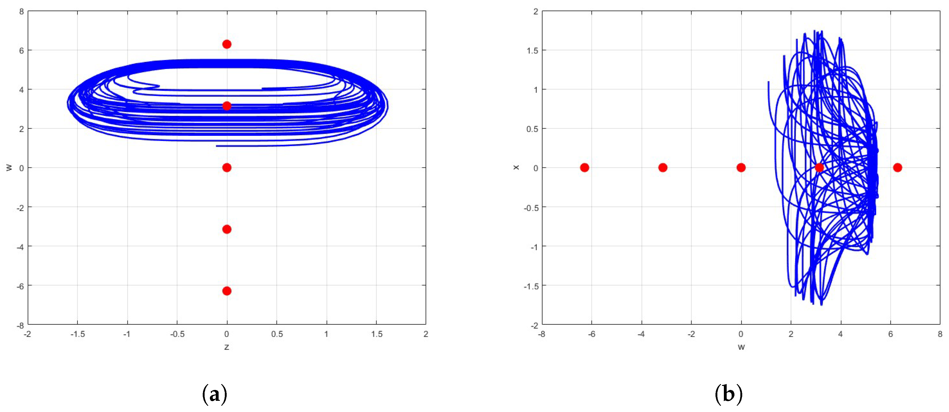
Symmetry and Invariance

It is obvious that system (1) is invariant under transformation $(x,y,z,w)\to (-x,-y,z,w)$ and symmetric about the coordinate axis $z,w.$

The dissipativity of system (1) is expressed as

$$\begin{array}{c}\hfill \nabla V={\displaystyle \frac{\partial \dot{x}}{\partial x}}+{\displaystyle \frac{\partial \dot{y}}{\partial y}}+{\displaystyle \frac{\partial \dot{z}}{\partial z}}+{\displaystyle \frac{\partial \dot{w}}{\partial w}}=-z^3.\end{array}$$

(5)

From (5), it is not clear how to determine the dissipativity when $\nabla V=-z^3\left(t\right)$ as $t\to \infty$. Therefore, we investigate $\nabla V$ numerically using the following formula, as proposed in [22,23]. The average value of $q\left(t\right)$ defined by

$$\begin{array}{c}\hfill \overline{q}\left(t\right)=\underset{t\to \infty }{lim}\left({\int }_{t_0}^{t}q\left(t\right)dt/t-t_0\right).\end{array}$$

(6)

By Formula (6), we discover that the average value $-z^3\left(t\right)\approx 0$ and the system (1) are conservative. Figure 1 shows the average of $z^3\left(t\right)=0.09571$ for $t=2000$. In particular, $\nabla V=trac\left(J\left({\mathbf{E}}_{\mathbf{IM}}\right)\right)=\mathbf{0}.$

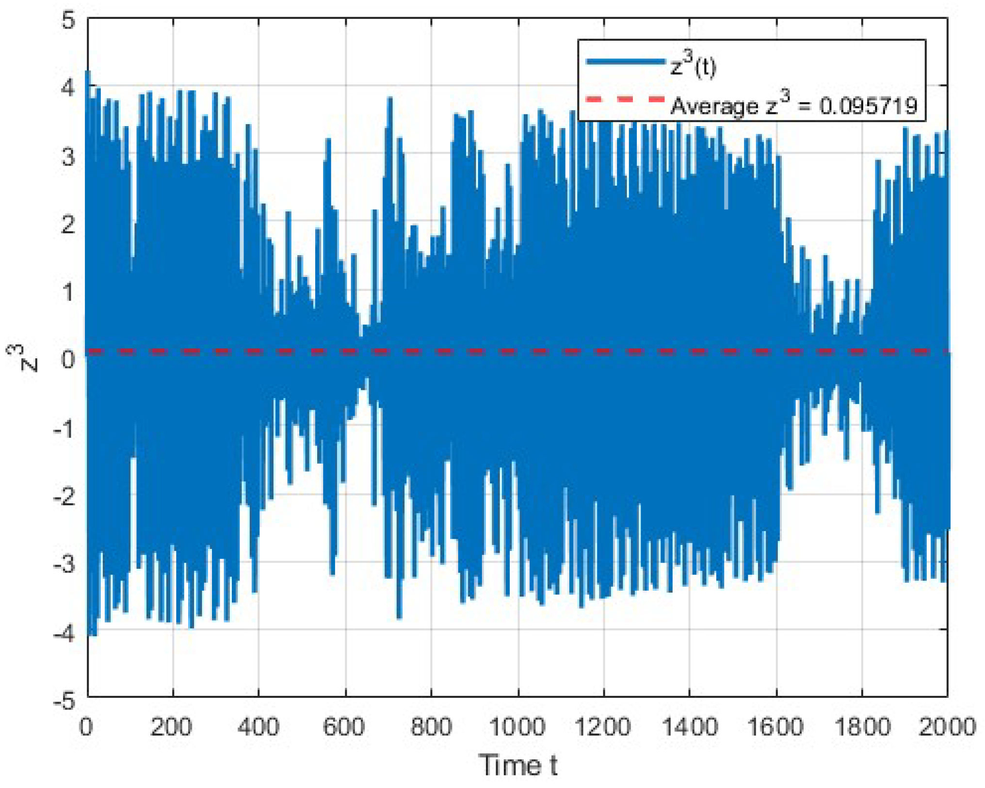
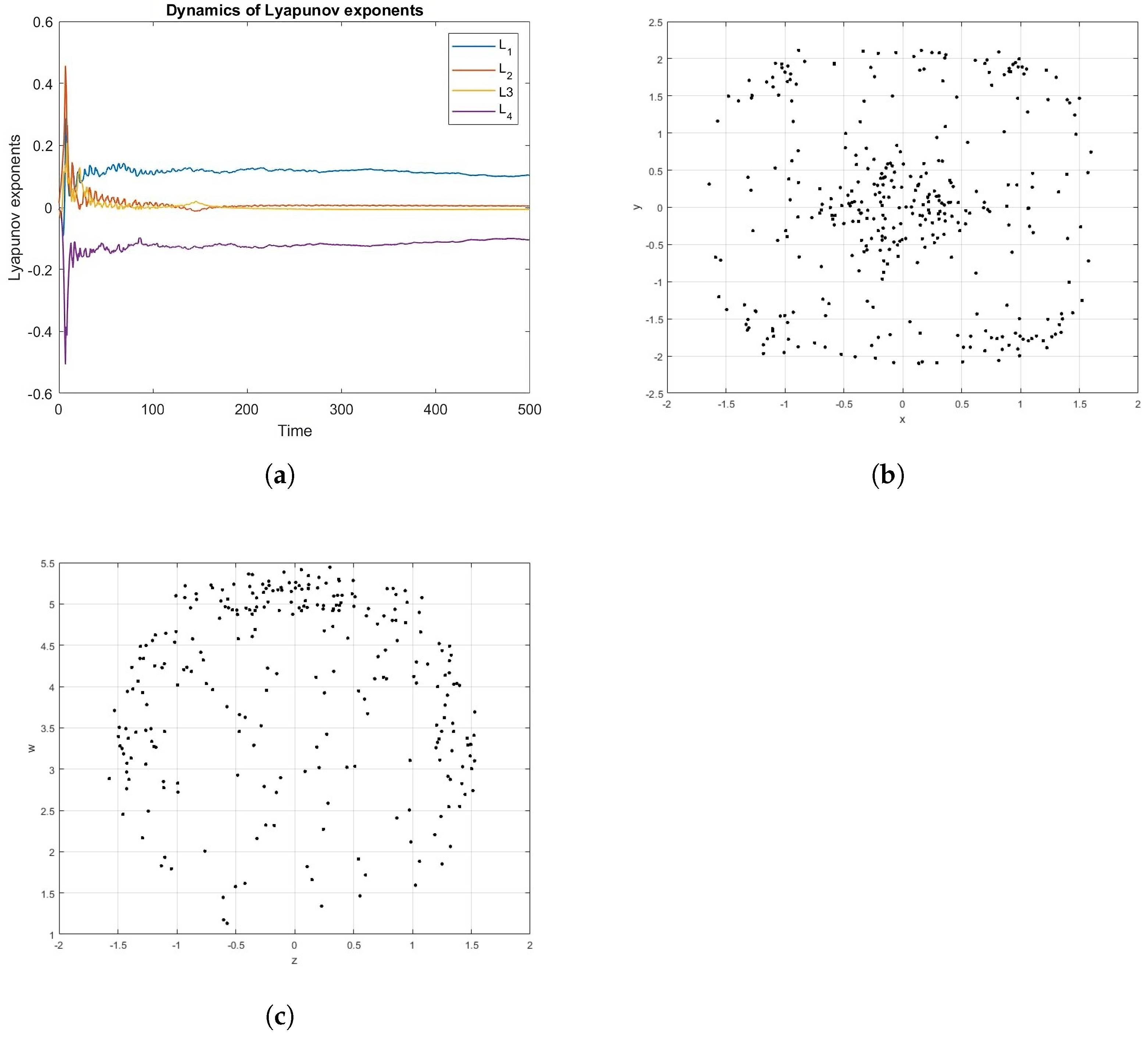
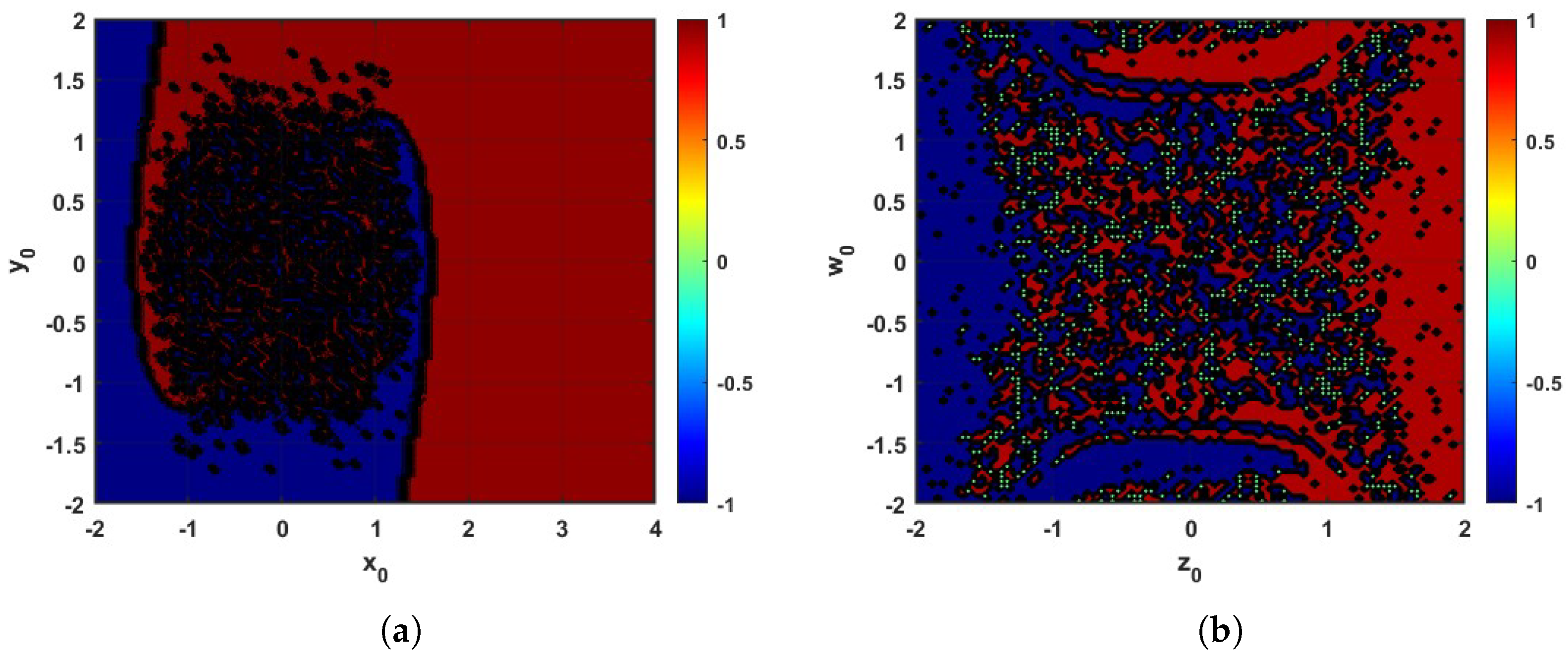
4. Dynamical Analysis

In this section, the fourth-order Runge–Kutta algorithm programmed in MATLAB ode45 is used for numerical simulations. Taking into account the value of a typical parameter of $\alpha =1.3$ and the initial condition (IC) of $(-0.11, 0.11, 0.11, -0.11)$, the system described by (1) exhibits complex dynamics, such as hyperchaos as shown in Figure 2. By applying Wolf’s method [37] and considering a time length of 500 s and testing the behavior of the trajectories, the four finite-time Lyapunov exponents are calculated as $L_1=0.038$, $L_2=0.01$, $L_3=-0.01$, and $L_4=-0.038$, where ${\sum }_{k=1}^4{L}_k=0$. The corresponding Kaplan–Yorke dimension ($D_{\mathrm{KY}}$) is then calculated as below:

$$\begin{array}{c}\hfill D_{\mathrm{KY}}=K+{\displaystyle \frac{1}{|L_{K+1}|}}\sum _{j=1}^K{L}_j,\end{array}$$

(7)

where K is the largest integer matches ${\sum }_{j=1}^K{L}_j\ge 0$ and ${\sum }_{j=1}^{K+1}{L}_j<0$. Consequently, $D_{\mathrm{KY}}$ is determined to be 4, indicating the presence of a strange attractor. This observation highlights the conservative nature of the proposed system, given that the dimension matches the dimensionality of the system. Figure 2a–d display projections and phase trajectories of the system (1) in various planes, the red dots are the equilibrium points $(0,0,0,n\pi )$ where $n=-2,-1,0,1,2$.

The Lyapunov exponent curves are depicted in Figure 3a. Furthermore, Figure 3b,c illustrate the Poincaré sections on the $z-w$ plane while $x=y=0$ and the $x-y$ plane during $z=w=0$ next reach a steady state (i.e., $t>100$).

In addition, the analysis of attraction basins serves as an additional tool for investigating dynamics. Figure 4 shows the basins of attraction for the dynamics of the system (1) with $\alpha =1.3$, achieved by varying two initial conditions while maintaining the other two at zero. The basins of attraction are visualized in Figure 4a in the $x_0-y_0$ plane with $x_0\in [-2,4]$ and $y_0\in [-2,2]$, and in Figure 4b on the $z_0-w_0$ plane with $z_0\in [-2,2]$ and $w_0\in [-2,2]$. To prevent torus attractors, the intervals for the initial conditions are selected. The colors red and black correspond to periodic and chaotic solutions, respectively, with the colors representing periodic solutions encoding the period.

Moreover, the Hamiltonian function can be given as a positive definite energy function identified as follows:

$$\begin{array}{c}\hfill H={\displaystyle \frac{1}{4}}(a{x}^4+2a{y}^2+z^4)+cos\left(w\right)+1,\end{array}$$

(8)

Then,

$$\begin{array}{c}\hfill \dot{H}={\displaystyle \frac{\partial H}{\partial x}}\dot{x}+{\displaystyle \frac{\partial H}{\partial y}}\dot{y}+{\displaystyle \frac{\partial H}{\partial z}}\dot{z}+{\displaystyle \frac{\partial H}{\partial w}}\dot{w}=0\end{array}$$

(9)

It confirms that the system’s energy (1) is constant. As a result, the system is conservative by definition.

The Complexity of Parameters Variations

To determine the complexity of the dynamics, it is essential to visualize the behavior of the system over the wide interval of its parameter $\alpha$. In Figure 5a,b, we present the bifurcation diagram in two different intervals with keeping the initial conditions of the system as $x_0=-0.11,y_0=0.11,z_0=0.11,w_0=-0.11$. The bifurcation diagram illustrates the system’s evolution over the time interval $t\in$ [0, 10,000] based on the simulations conducted; system (1) can exhibit hyperchaotic and chaotic behaviors when the parameter is set suitably. As can be shown, the system provides two positive Lyapunov exponents in the interval $\alpha \in [0,60]$, although there are no chaotic attractors throughout $\alpha \in (60,75)$. We can as well see the chaotic attractor in the interval $[75,100]$; it is observed that in the parameter interval $[60,75]$, the system does not generate any meaningful or bounded trajectories. This may indicate a loss the nonlinear dynamic behavior. Consequently, this range is excluded from the bifurcation analysis due to the absence of attractors. Furthermore, in dynamical systems theory, one of the most fascinating topics is how to evaluate the system’s complexity over time. The thermodynamic idea of “entropy” in the 19th century became a crucial instrument for estimating the complexity of these kinds of system. Today, entropy remains a key idea in information theory, assisting with the analysis of chemical reactions and various other disciplines. Let $\rho$ signify the D-dimensional box in the state space with side length $\epsilon$ where $x_i$ is visible, and let ${\xi }_i$ represent the initial Poincaré recurrence times. We denote the probability distribution of ${\xi }_i$ as $\gamma (\xi ,\rho )$. The Kolmogorov–Sinai entropy is commonly known as

$$\begin{array}{c}\hfill H_{KSE}\left(\rho \left[\epsilon \right]\right)={\displaystyle \frac{1}{{\xi }_{min}\rho \left[\epsilon \right]}}\sum _{\xi }\gamma (\xi ,\rho \left[\epsilon \right])log\left({\displaystyle \frac{1}{\gamma (\xi ,\rho [\epsilon \left]\right)}}\right).\end{array}$$

(10)

For chaotic dynamics, Equation (10) is particularly high. Moreover, if the transitory time is not eliminated, approaching bifurcation sites can be found in the entropy. This occurs because the state becomes widely distributed at bifurcation points due to their inherent sluggishness.

Analysis of Figure 5a,b reveals that as the parameter $\alpha$ approaches 1, the Kolmogorov–Sinai entropy shows an increase in positive values within hyperchaotic regions. This indicates a high complexity in the hyperchaotic region of the system (1). In particular, in Figure 5c, the Kolmogorov–Sinai entropy is shown for $\alpha \in [0,1.5]$, with a step size of $\Delta \alpha =0.002$ and $t=500$.

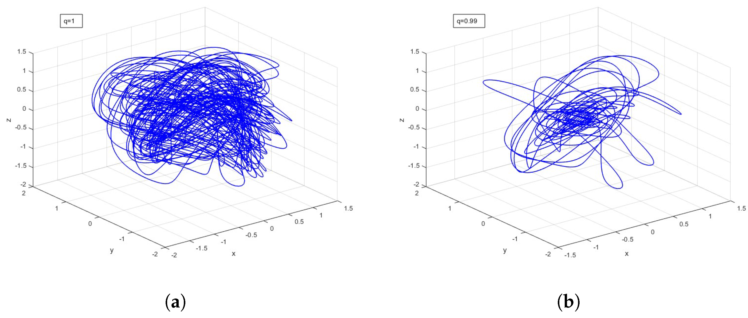
5. Fractional-Order for System (1)

In applications involving synchronization, circuit construction, and security, fractional-order systems exhibit strong capabilities. More stable synchronized states and stronger coupling between chaotic systems are made possible by their memory effects in synchronization. Fractional capacitors and other fractional-order components help circuit realizations by producing more complicated dynamics with fewer components. Their improved chaotic behavior and extra fractional parameters offer stronger encryption and improved attack resistance, which makes them particularly useful in secure communications. In addition, the Lyapunov exponents and phase profiles for a $4D$ conservative hyperchaotic system are determined in this work, which builds on previous studies on fractional-order chaotic systems, helping to characterize high-dimensional dynamics theoretically. Applications such as synchronization and secure communication have been the subject of numerous studies [29,38,39], helping to theoretically characterize high-dimensional dynamics. Specifically, the use of the Grünwald–Letnikov (GL) approach for the computation of the Lyapunov exponent, as rigorously derived in [33], ensures precision in the capture of long-memory effects, a feature emphasized in [40] for its broader chaotic range. The analytical method used here is supported by the theoretical foundation for fractional dynamical systems developed in [41], especially in linearization and stability evaluation. This paper analyzes explicit hyperchaotic attractors in a conservative system, exposing different dynamical features from [42], which studies hidden attractors in incommensurate-order systems. The bifurcation and phase portrait analyses are parallel [29,43] yet differentiated by focusing on conservatives, a less explored feature compared to dissipative systems. Although parameter sensitivity and order-dependent chaotic ranges are highlighted in [44,45], respectively, they show how fractional-order dynamics maintain hyperchaos even when order is reduced, supporting the findings of [45] about contraction effects. Although previous work has focused mainly on synchronization control techniques [29,38,39], the lack of these applications here highlights a conscious move towards basic dynamics, bridging a gap between theoretical developments [33,41,46,47] and applied research. By highlighting the novelty of describing a $4D$ conservative hyperchaotic system, the result goes beyond previous research to understand complex fractional-order behaviors.

In this part, the theoretical and computational components of the topic mentioned above are addressed. Fractional calculus, an extension of integration and differentiation for non-integer orders, is represented through the continuous integro-differential operator ${}_{b}D_t^q$. This operator can be expressed as follows:

$$\begin{array}{c}\hfill b{D}_t^q=\left\{\begin{array}{c}{\mathrm{d}}^q/\mathrm{d}{t}^{q}q>0\hfill \\ 1q=0\hfill \\ {\int }_b^t{\left(ds\right)}^{q}q<0\hfill \end{array}\right.\end{array}$$

(11)

The main fractional-order operator is defined by three commonly used definitions: the Riemann–Liouville operator (RLO), the Caputo operator (CO), and the Grunwald–Letnikov operator (GLO) [48]. Moreover, the method of the GLO definition can be utilized to construct the numerical framework for (1). Subsequently, the forward and backward derivatives can be established, with our focus solely on the forward derivative. In [49,50], the forward GLO derivative for a function $X\left(t\right)$ with order q is expressed as

$$\begin{array}{c}\hfill D_f^{q}X\left(t\right)=\underset{\left|h\right|\to 0}{lim}{\displaystyle \frac{{\sum }_{k=0}^{\infty }{(-1)}^k\left(\genfrac{}{}{0pt}{}{q}{k}\right)X(t-kh)}{{\left|h\right|}^q}}.\end{array}$$

(12)

With the Grunwald–Letnikov fractional-order operator denoted by $GL$ (refer to [48,51]) is the fractional-order dynamical differential equation of system (1), which is defined as

$$\left\{\begin{array}{cc}{D}_t^{q}x\hfill & =y,\hfill \\ D_t^{q}y\hfill & =-x^3-y{z}^3,\hfill \\ D_t^{q}z\hfill & =\alpha y^2+sinw,\hfill \\ D_t^{q}w\hfill & =z^3,\hfill \end{array}\right.$$

(13)

Assume that the summation in (12) is confined to ${\displaystyle \frac{t-a}{h}}$, where $a>0$. Then, we have

$$\begin{array}{c}\hfill D_f^{q}X\left(t\right)=\underset{\left|h\right|\to 0}{lim}{\displaystyle \frac{{\sum }_{k=0}^{\lfloor \frac{t-a}{h}\rfloor }{(-1)}^k\left(\genfrac{}{}{0pt}{}{q}{k}\right)X(t-kh)}{{\left|h\right|}^q}},\end{array}$$

(14)

where the integer component of ${\displaystyle \frac{t-a}{h}}$ is the greatest integer: $\lfloor 1.2\rfloor =1$, $\lfloor 4.6\rfloor =4$. The following represents the specific numerical estimation of the $q^{th}$ derivative at the points $lh=1,2,...$ and takes the following form:

$$\begin{array}{c}\hfill {}_{{\displaystyle {\displaystyle \frac{l-L_m}{h}}}}D_{t_l}^{q}X\left(t\right)=h^{-q}\sum _{k=0}^l{(-1)}^k\left({\displaystyle \genfrac{}{}{0pt}{}{q}{k}}\right)X\left(t_{l-k}\right),\end{array}$$

(15)

where $L_m$ is the memory length, $t_l=lh$ is the time step, and ${(-1)}^k\left({\displaystyle \genfrac{}{}{0pt}{}{q}{k}}\right)$ is the binomial coefficients $C_k^q$. Thus, in [43,52], one can find $C_0^q=1$ and $C_k^q=1-{\displaystyle \frac{1+q}{k}}{C}_{k-1}^q.$

The forward difference method, a widely used technique for approximating derivatives in fractional-order systems, allows the system in Equation (13) to be expressed as

$$\left\{\begin{array}{cc}{D}_t^{q}x\hfill & =h^{-q}{\displaystyle \sum _{k=1}^l}{C}_k^q{x}_{(l-k)}=y,\hfill \\ D_t^{q}y\hfill & =h^{-q}{\displaystyle \sum _{k=1}^l}{C}_k^q{y}_{(l-k)}=-x^3-y{z}^3,\hfill \\ D_t^{q}z\hfill & =h^{-q}{\displaystyle \sum _{k=1}^l}{C}_k^q{z}_{(l-k)}=\alpha y^2+sinw,\hfill \\ D_t^{q}w\hfill & =h^{-q}{\displaystyle \sum _{k=1}^l}{C}_k^q{w}_{(l-k)}=z^3.\hfill \end{array}\right.$$

(16)

Now, let us express the solution of a fractional-order system (16) as

$$\begin{array}{cc}\hfill x_{\left(k\right)}& =\left(y_{(k-1)}\right)h^q-\sum _{k=1}^l{C}_k^q{x}_{(l-k)}\hfill \\ \hfill y_{\left(k\right)}& =(-x_{\left(k\right)}^3-y_{(k-1)}{z}_{(k-1)}^3)h^q-\sum _{k=1}^l{C}_k^q{y}_{(l-k)}\hfill \\ \hfill z_{\left(k\right)}& =(y_{\left(k\right)}^2+sin\left(w_{(k-1)}\right))h^q-\sum _{k=1}^l{C}_k^q{z}_{(l-k)}\hfill \\ \hfill w_{\left(k\right)}& =\left(z_{\left(k\right)}^3\right)h^q-\sum _{k=1}^l{C}_k^q{w}_{(l-k)}\hfill \end{array}$$

(17)

5.1. Existence of a Unique Solution

It is well known that the system model has a unique solution if the Lipschitz continuity of the kernels is satisfied. The first step involves converting the Grunwald–Letnikov GL operator to the Caputo operator’s fractional order of the system. The system based on the Caputo operator is as follows:

$$\left\{\begin{array}{cc}{B}_t^{q}x\hfill & =y,\hfill \\ B_t^{q}y\hfill & =-x^3-y{z}^3,\hfill \\ B_t^{q}z\hfill & =\alpha y^2+sinw,\hfill \\ B_t^{q}w\hfill & =z^3.\hfill \end{array}\right.$$

(18)

The Banach space $\mathbf{S}\left(\right[0,T\left]\right)$ is defined using the norm $\left|x\left(k\right)\right|={sup}_k\left|x\left(k\right)\right|$. Now, we establish a Banach space, $\psi =\mathbb{S}\left(U\right)\times \mathbb{S}\left(U\right)\times \mathbb{S}\left(U\right)\times \mathbb{S}\left(U\right)$, with the norm $\parallel x+y+z+w\parallel \le \parallel x\parallel +\parallel y\parallel +\parallel z\parallel +\parallel w\parallel$, where $\parallel x\parallel ={sup}_t\left|x\left(t\right)\right|$, $\parallel y\parallel ={sup}_t\left|y\left(t\right)\right|$, $\parallel z\parallel ={sup}_t\left|z\left(t\right)\right|$, and $\parallel w\parallel ={sup}_t\left|w\left(t\right)\right|$. The system (18) can be expressed as

$$\left\{\begin{array}{cc}{D}_t^{q}x\hfill & =B_1(t,x)=y,\hfill \\ D_t^{q}y\hfill & =B_2(t,y)=-x^3-y{z}^3,\hfill \\ D_t^{q}z\hfill & =B_3(t,z)=\alpha y^2+sinw,\hfill \\ D_t^{q}w\hfill & =B_4(t,w)=z^3,\hfill \end{array}\right.$$

(19)

From (19), we can write the following as

$$\left\{\begin{array}{cc}x\left(t\right)\hfill & =x_0+{\displaystyle \frac{1}{\Gamma \left(q\right)}}{\int }_0^t{(t-s)}^{q-1}{B}_1(s,x)ds,\hfill \\ y\left(t\right)\hfill & =y_0+{\displaystyle \frac{1}{\Gamma \left(q\right)}}{\int }_0^t{(t-s)}^{q-1}{B}_2(s,y)ds,\hfill \\ z\left(t\right)\hfill & =z_0+{\displaystyle \frac{1}{\Gamma \left(q\right)}}{\int }_0^t{(t-s)}^{q-1}{B}_3(s,z)ds,\hfill \\ w\left(t\right)\hfill & =w_0+{\displaystyle \frac{1}{\Gamma \left(q\right)}}{\int }_0^t{(t-s)}^{q-1}{B}_4(s,w)ds.\hfill \end{array}\right.$$

(20)

Suppose $x,x_1;$$y,y_1;z,z_1$ and $w,w_1$ are the solutions of (19), to demonstrate that the kernels satisfy the Lipschitz condition, we apply the Banach fixed point theorem only to system (20) as follows:

$$\left\{\begin{array}{c}\parallel B_1(s,x)-B_1(s,x_1)\parallel =\parallel y-y_1\parallel \le {\eta }_1\parallel (y-y_1)\parallel ;\hfill \\ \parallel B_2(s,y)-B_2(s,y_1)\parallel =\parallel (-x^3-y{z}^3)-(-x_1^3-y_1{z}_1^3)\parallel \le {\eta }_2\parallel x-x_1\parallel +\parallel y-y_1\parallel +\parallel z-z_1\parallel ;\hfill \\ \parallel B_3(s,z)-B_3(s,z_1)\parallel =\parallel (a{y}^3+sin\left(w\right))-(a{y}_1^3+sin\left(w_1\right))\parallel \le {\eta }_3\parallel y-y_1\parallel +\parallel w-w_1\parallel ;\hfill \\ \parallel B_4(s,w)-B_4(s,w_1)\parallel =\parallel z^3-z_1^3\parallel \le {\eta }_4\parallel z-z_1\parallel \hfill \end{array}\right.$$

(21)

where

$$\left\{\begin{array}{cc}{\eta }_1=\left|1\right|;\hfill & \\ {\eta }_2=max\left\{\right|x^{+}x{x}_1+x_1^2|,|z_1^3|,|y\left|\right\};\hfill & \\ {\eta }_3=max\left\{\right|y^2+y{y}_1+y_1^3|,|2cos\left({\displaystyle \frac{w+w_1}{2}}\right)\left|\right\};\hfill & \\ {\eta }_4=max\left\{\right|z^2+z{z}_1+z_1^2\left|\right\}.\hfill \end{array}\right.$$

Thus, for $max|{\eta }_i|,i=1,2,3,4$, the kernels $B_1(s,x),B_2(s,y),B_3(s,z),B_4(s,w)$ in (21) satisfy the contraction condition.

Equation (20) can be expressed as follows:

$$\left\{\begin{array}{cc}x{\left(t\right)}_h\hfill & =x_0+{\displaystyle \frac{1}{\Gamma \left(q\right)}}{\int }_0^t{(t-s)}^{q-1}{B}_1(s,x_{h-1})ds,\hfill \\ y{\left(t\right)}_h\hfill & =y_0+{\displaystyle \frac{1}{\Gamma \left(q\right)}}{\int }_0^t{(t-s)}^{q-1}{B}_2(s,y_{h-1})ds,\hfill \\ z{\left(t\right)}_h\hfill & =z_0+{\displaystyle \frac{1}{\Gamma \left(q\right)}}{\int }_0^t{(t-s)}^{q-1}{B}_3(s,z_{h-1})ds,\hfill \\ w{\left(t\right)}_h\hfill & =w_0+{\displaystyle \frac{1}{\Gamma \left(q\right)}}{\int }_0^t{(t-s)}^{q-1}{B}_4(s,w_{h-1})ds,\hfill \end{array}\right.$$

(22)

Based on the previous equations, we get the following:

$$\left\{\begin{array}{cc}{\Delta }_{1}x{\left(t\right)}_h\hfill & =x_h-x_{h-1}={\displaystyle \frac{1}{\Gamma \left(q\right)}}{\int }_0^t{(t-s)}^{q-1}[B_1(s,x_{h-1})-B_1(s,x_{h-2})]ds,\hfill \\ {\Delta }_{2}y{\left(t\right)}_h\hfill & =y_h-y_{h-1}={\displaystyle \frac{1}{\Gamma \left(q\right)}}{\int }_0^t{(t-s)}^{q-1}\left[B_2(s,y_{h-1}-B_2(s,y_{h-2})]\right)ds,\hfill \\ {\Delta }_{3}z{\left(t\right)}_h\hfill & =z_h-z_{h-1}={\displaystyle \frac{1}{\Gamma \left(q\right)}}{\int }_0^t{(t-s)}^{q-1}[B_3(s,z_{h-1}-B_3(s,z_{h-2})]ds,\hfill \\ {\Delta }_{4}w{\left(t\right)}_h\hfill & =w_h-w_{h-1}={\displaystyle \frac{1}{\Gamma \left(q\right)}}{\int }_0^t{(t-s)}^{q-1}[B_4(s,w_{h-1})-B_4(s,w_{h-2})]ds,\hfill \end{array}\right.$$

(23)

By taking the norm to ${\Delta }_{1}x{\left(t\right)}_h$ in (23), we obtain align

$$\begin{array}{cc}\hfill \parallel {\Delta }_{1}x{(t)}_h\parallel & =\parallel x_h-x_{h-1}\parallel \hfill \\ \hfill & =\parallel {\displaystyle \frac{1}{\mathsf{\Gamma }(q)}}{{\displaystyle \int }}_0^t{(t-s)}^{q-1}\left[B_1\left(s,x_{h-1}\right)-B_1\left(s,x_{h-2}\right)\right]ds\parallel \hfill \\ \hfill & \le {\displaystyle \frac{1}{\mathsf{\Gamma }(q)}}{{\displaystyle \int }}_0^t{(t-s)}^{q-1}\parallel B_1\left(s,x_{h-1}\right)-B_1\left(s,x_{h-2}\right)\parallel ds\hfill \\ & \le {\displaystyle \frac{{\gamma }_1}{\mathsf{\Gamma }(q)}}{{\displaystyle \int }}_0^t{(t-s)}^{q-1}\parallel x-x_1\parallel ds,\hfill \\ \hfill \parallel {\varphi }_{1h}\parallel & \le {\displaystyle \frac{{\gamma }_1}{\mathsf{\Gamma }(q)}}{{\displaystyle \int }}_0^t{(t-s)}^{q-1}\parallel {\varphi }_{1h-1}\parallel ds.\hfill \end{array}$$

(24)

Applying the same techniques as considered in (24) to ${\Delta }_{2}y{\left(t\right)}_h,{\Delta }_{3}z{\left(t\right)}_h,{\Delta }_{4}w{\left(t\right)}_h$ in (23), we get the following:

$$\left\{\begin{array}{cc}\parallel {\varphi }_{2h}\parallel \hfill & \le {\displaystyle \frac{{\gamma }_2}{\Gamma \left(q\right)}}{\int }_0^t{(t-s)}^{q-1}\parallel {\varphi }_{2h-1}\parallel ds.\hfill \\ \parallel {\varphi }_{3h}\parallel \hfill & \le {\displaystyle \frac{{\gamma }_3}{\Gamma \left(q\right)}}{\int }_0^t{(t-s)}^{q-1}\parallel {\varphi }_{3h-1}\parallel ds.\hfill \\ \parallel {\varphi }_{4h}\parallel \hfill & \le {\displaystyle \frac{{\gamma }_4}{\Gamma \left(q\right)}}{\int }_0^t{(t-s)}^{q-1}\parallel {\varphi }_{4h-1}\parallel ds.\hfill \end{array}\right.$$

(25)

Hence,

$$\left\{\begin{array}{c}{x}_h\left(t\right)={\displaystyle \sum _{i=1}^h}{\varphi }_{1i}\left(t\right),y_h\left(t\right)={\displaystyle \sum _{i=1}^h}{\varphi }_{2i}\left(t\right)\hfill \\ z_h\left(t\right)={\displaystyle \sum _{i=1}^h}{\varphi }_{3i}\left(t\right),w_h\left(t\right)={\displaystyle \sum _{i=1}^h}{\varphi }_{4i}\left(t\right)\hfill \end{array}\right.$$

(26)

Analyzing the model shows only one solution.

5.2. Low Effective Order

Here, we present a numerical simulation of system (1) with commensurate fractional orders. We observe chaotic behavior that arises upon the application of the fractional-order derivative. A comparison of the geometries of the attractors is used to analyze and demonstrate the influence of the fractional-order operator according to the modification of the $GL$ operator. Therefore, we set the initial conditions to $(-0.11,0.11,0.11,-0.11)$, a step size of $0.05$, a time $t=500$, and a value of $\alpha =1.3$. Different attractor forms are achieved by changing the order q while keeping the value of the parameter $\alpha$. The chaotic motion in the fractional Equation (13) appears when the orders of the fractional derivatives vary within the interval $[0.93,1)$. Furthermore, the sum of all Lyapunov exponents is nearly zero, indicating that the system preserves its conservatism. The computed Lyapunov exponents in

Table 2. The Lyapunov exponents for fractional-order system (16) to a commensurate order with different values of q where ↓ shows that as much the order q approach zero, the fractional-order system (16) became chaotic.

Order (q)	${\mathit{L}}_1$	${\mathit{L}}_2$	${\mathit{L}}_3$	${\mathit{L}}_4$	${\sum }_{\mathit{i}=1}^4{\mathit{L}}_{\mathit{i}}$	Kaplan–Yorke
1 ↓	0.0919	0.0045	0	−0.0982	−0.0125	3.865 ≃ 4 ↓
0.99 ↓	0.0081	0.0149	0	−0.0343	−0.0218	3.364 ↓
0.98 ↓	0.0104	0.0077	0	−0.0357	−0.0365	2.958↓
0.97 ↓	0.0085	0	−0.0013	−0.0330	−0.0458	2.360 ↓
0.96 ↓	0.0097	0	−0.0040	−0.0468	−0.0600	2.301 ↓
0.95↓	0.0092	0	−0.0038	−0.0512	−0.0746	2.188 ↓
0.94 ↓	0.0008	0	−0.0055	−0.0583	−0.0923	1.145 ↓
0.93 ↓	0.0021	0	−0.0181	−0.0669	−0.0112	1.116 ↓

indicate that the new system exhibits hyperchaotic behavior. In the solutions of the fractional-order system, when the fractional orders fall within the interval $[0.98,1)$, two positive, one negative, and one zero of the Lyapunov exponent exist. The fractional-order system (13) is chaotic for $q\in (98,93]$. Furthermore, the Kaplan–Yorke value, as shown in Table 2, decreases as the order decreases, highlighting that the chaotic characteristics decrease as the order decreases.

We observe Figure 6 displayed in various orders: in $\left(a\right)$, we observe the trajectory of the hyperchaotic system (13)—its order is one. Then, $\left(b\right)$ displays the fractional-order hyperchaotic system’s dynamics displayed with order $0.99$. As can be observed in $\left(c\right)$, the hyperchaotic behavior is preserved, and so on until k with order $0.93$ moves into a weakness of chaos. However, when $1\le q<0.97$, system (13) generates hyperchaotic behavior, whereas for all orders $q\in [0.97,1]$, the system saves the chaotic behavior because chaos is sensitive to the initial condition, which can be examined. This phase trajectory definitely shows that order reduction does not remove the oscillator’s chaotic behavior. Figure 6 shows a quantifiable relationship between the physical density of chaotic trajectories in the dynamical system and the order parameter. The phase space figures show an increase in trajectory density at the highest order $\left(1.0\right)$, which is a sign of strong chaotic behavior. A significant decrease in trajectory density is shown when the order parameter gradually drops to 0.93, indicating a decrease in the complexity of the system’s fractal structures.

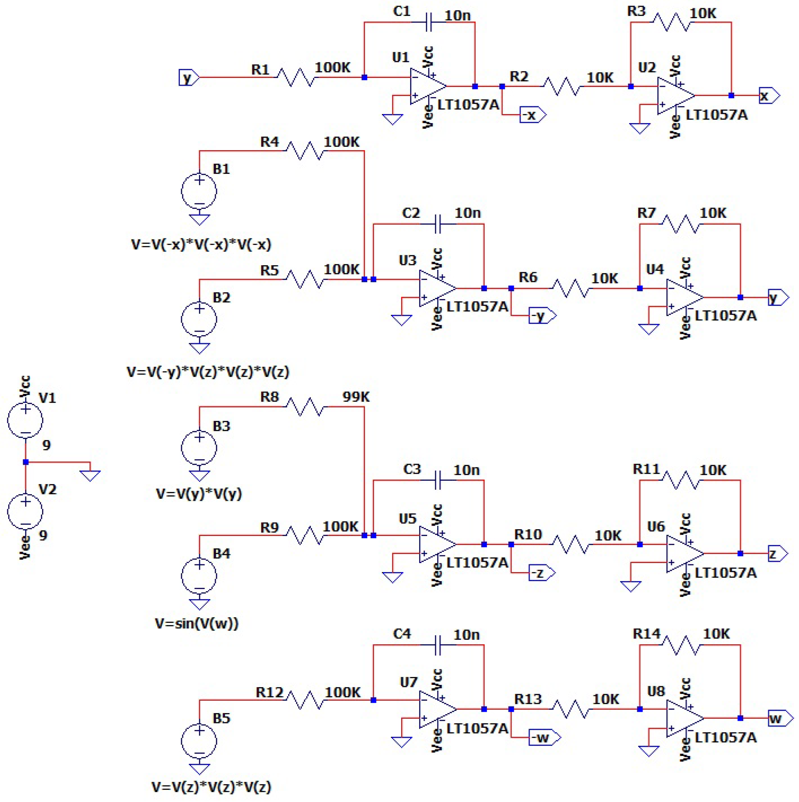
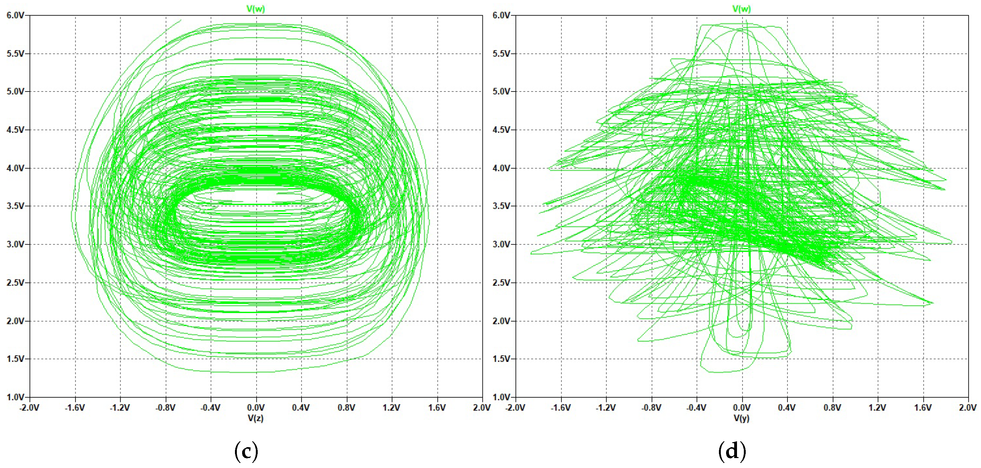
6. Hardware Implementation

We built an analog circuit for system (1) to validate the results of the previous numerical simulations using LTspice, as indicated by

$$\left\{\begin{array}{cc}X={\displaystyle \frac{1}{R_1{C}_1}}y,\hfill & \\ Y=-{\displaystyle \frac{1}{R_2{C}_2}}{x}^3-{\displaystyle \frac{1}{R_3{C}_3}}y{z}^3,\hfill & \\ Z={\displaystyle \frac{1}{R_4{C}_4}}\alpha y^2+{\displaystyle \frac{1}{R_5{C}_5}}sinw,\hfill & \\ W={\displaystyle \frac{1}{R_6{C}_6}}{z}^3,\hfill \end{array}\right.$$

where the environment is provided in Figure 7. The four state variables are implemented using four integrators (LT1057A). Additionally, a sinusoidal voltage generator is engaged. Operational amplifiers (OpAmps) are the basis of the integrator circuit design. The values of the capacitors are set as $C_1=C_2=C_3=10$ nF; and the resistors are determined as $R_1=R_4=R_5=R_9=R_{12}=100$ kΩ; $R_8=99$ kΩ, $R_2=R_3=R_6=R_7=R_{10}=R_{11}=R_{13}=R_{14}=10$ kΩ. Moreover, the supply voltages for the OpAmps are specified as $V_{cc}=9$ V and $V_{ee}=9$ V.

The experimental results obtained from the physical circuit closely match the simulation results, as shown in Figure 8. The system exhibits the expected chaotic behavior, with attractors projected onto various plane axes with the initial condition $(x_0;y_0;z_0;w_0)=(-0.11;0.11;0.11;-0.11)$. These results demonstrate that the analog circuit successfully replicates the system dynamics, confirming the feasibility of the proposed design.

7. Conclusions

This paper presents a novel four-dimensional conservative hyperchaotic system characterized by an infinite number of equilibrium points, all associated with a Jacobian matrix whose eigenvalues are identically zero. Due to this complete degeneracy, the classical linear stability theory is inapplicable; instead, a combination of analytical and numerical techniques confirms that the system is locally stable around each equilibrium point.

The system conserves energy within a bounded region of phase space and exhibits rich hyperchaotic dynamics. These dynamics are characterized using various diagnostic tools, including Lyapunov exponents, bifurcation diagrams, parameter sensitivity analysis, attractor projections, and Poincaré cross sections.

Furthermore, the system is extended to the fractional-order domain using the non-integer Grünwald–Letnikov operator, ${}_{b}D_t^q$, which reveals additional complexity and memory-dependent behavior. To support the theoretical and numerical results, an analog circuit implementation of the integer-order case was developed and simulated, demonstrating practical realizability.

The proposed system not only expands the catalog of known conservative hyperchaotic systems but also opens avenues for future research in stability theory for degenerate systems and fractional-order nonlinear dynamics.

References

1. Lorenz, E.N. Deterministic nonperiodic flow. J. Atmos. Sci. 1963, 20, 130–141. [Google Scholar] [CrossRef]
2. Rössler, O.E.; Letellier, C. Chaos: The World of Nonperiodic Oscillations; Springer Nature: Berlin/Heidelberg, Germany, 2020. [Google Scholar]
3. Jafari, S.; Sprott, J.; Nazarimehr, F. Recent new examples of hidden attractors. Eur. Phys. J. Spec. Top. 2015, 224, 1469–1476. [Google Scholar] [CrossRef]
4. Leonov, G.; Kuznetsov, N.; Vagaitsev, V. Localization of hidden Chua’s attractors. Phys. Lett. A 2011, 375, 2230–2233. [Google Scholar] [CrossRef]
5. Cang, S.; Li, Y.; Zhang, R.; Wang, Z. Hidden and self-excited coexisting attractors in a Lorenz-like system with two equilibrium points. Nonlinear Dyn. 2019, 95, 381–390. [Google Scholar] [CrossRef]
6. Yu, T.; Ma, W.; Wang, Z.; Li, X. Hidden and self-excited attractors in an extended Sprott C system with two symmetric or asymmetric equilibrium points. Eur. Phys. J. Spec. Top. 2023, 96, 1287–1299. [Google Scholar] [CrossRef]
7. Shukur, A.A.; AlFallooji, M.A.; Pham, V.T. Asymmetrical novel hyperchaotic system with two exponential functions and an application to image encryption. Nonlinear Eng. 2024, 13, 20220362. [Google Scholar] [CrossRef]
8. Tayyab, M.; Sun, K.; Yao, Z.; Wang, H. Dynamics of memristive Liu system and its DSP implementation. Phys. Scr. 2024, 99, 085273. [Google Scholar] [CrossRef]
9. Wang, X.; Chen, G. Constructing a chaotic system with any number of equilibria. Nonlinear Dyn. 2013, 71, 429–436. [Google Scholar] [CrossRef]
10. Pham, V.T.; Jafari, S.; Wang, X.; Ma, J. A chaotic system with different shapes of equilibria. Int. J. Bifurc. Chaos 2016, 26, 1650069. [Google Scholar] [CrossRef]
11. Strogatz, S. Nonlinear Dynamics and Chaos: With Applications to Physics Biology Chemistry and Engineering; Westview Press: Boulder, CO, USA, 2000. [Google Scholar]
12. Minati, L. Simulation versus experiment in non-linear dynamical systems. Chaos Solitons Fractals 2021, 144, 110656. [Google Scholar] [CrossRef]
13. Fatemeh, P.; Karthikeyan, R.; Anitha, K.; Ahmed, A.; Tasawar, H.; Viet-Thanh, P. Complex dynamics of a neuron model with discontinuous magnetic induction and exposed to external radiation. Cogn. Neurodyn. 2018, 12, 607–614. [Google Scholar] [CrossRef]
14. Yang, Y.; Ma, J.; Xu, Y.; Jia, Y. Energy dependence on discharge mode of Izhikevich neuron driven by external stimulus under electromagnetic induction. Cogn. Neurodyn. 2021, 15, 265–277. [Google Scholar] [CrossRef]
15. Xu, Q.; Wang, Y.; Chen, B.; Li, Z.; Wang, N. Firing pattern in a memristive Hodgkin-Huxley circuit: Numerical simulation and analog circuit validation. Chaos Solitons Fractals 2023, 172, 113627. [Google Scholar] [CrossRef]
16. Sajad, J.; Sprott, J.S.; Golpayegani, S. Elementary quadratic chaotic flows with no equilibria. Phys. Lett. A 2013, 377, 102–108. [Google Scholar] [CrossRef]
17. Wang, X.; Chen, G. A chaotic system with only one stable equilibrium. Commun. Nonlinear Sci. Numer. Simul. 2012, 17, 1264–1272. [Google Scholar] [CrossRef]
18. Jafari, S.; Sprott, J. Simple chaotic flows with a line equilibrium. Chaos Solitons Fractals 2013, 57, 79–84. [Google Scholar] [CrossRef]
19. Rajagopal, K.; Karthikeyan, A.; Srinivasan, A. Bifurcation and chaos in time delayed fractional order chaotic oscillator and its sliding mode synchronization with uncertainties. Chaos Solitons Fractals 2017, 103, 347–356. [Google Scholar] [CrossRef]
20. Yu, F.; Wang, C. A novel three dimension autonomous chaotic system with a quadratic exponential nonlinear term. Eng. Technol. Appl. Sci. Res. 2012, 2, 209–215. [Google Scholar] [CrossRef]
21. Neamah, A.A.; Shukur, A.A. A novel conservative chaotic system involved in hyperbolic functions and its application to design an efficient colour image encryption scheme. Symmetry 2023, 15, 1511. [Google Scholar] [CrossRef]
22. Zhang, X.; Chen, M.; Wang, Y.; Tian, H.; Wang, Z. Dynamic Analysis and Degenerate Hopf Bifurcation-Based Feedback Control of a Conservative Chaotic System and Its Circuit Simulation. Complexity 2021, 2021, 5576353. [Google Scholar] [CrossRef]
23. Singh, J.P.; Roy, B.K. Five new 4-D autonomous conservative chaotic systems with various type of non-hyperbolic and lines of equilibria. Chaos Solitons Fractals 2018, 114, 81–91. [Google Scholar] [CrossRef]
24. Mahmoud, G.M.; Ahmed, M. Analysis of chaotic and hyperchaotic conservative complex nonlinear systems. Miskolc Math. Notes 2017, 18, 315–326. [Google Scholar] [CrossRef]
25. Faghani, Z.; Nazarimehr, F.; Jafari, S.; Sprott, J.C. A new category of three-dimensional chaotic flows with identical eigenvalues. Int. J. Bifurc. Chaos 2020, 30, 2050026. [Google Scholar] [CrossRef]
26. ur Rahman, M.; El-Shorbagy, M.; Alrabaiah, H.; Baleanu, D.; De la Sen, M. Investigating a new conservative 4-dimensional chaotic system. Results Phys. 2023, 53, 106969. [Google Scholar] [CrossRef]
27. Zolfaghari-Nejad, M.; Charmi, M.; Hassanpoor, H. A new chaotic system with only nonhyperbolic equilibrium points: Dynamics and its engineering application. Complexity 2022, 2022, 4488971. [Google Scholar] [CrossRef]
28. Chen, L.; Nazarimehr, F.; Jafari, S.; Tlelo-Cuautle, E.; Hussain, I. Investigation of early warning indexes in a three-dimensional chaotic system with zero eigenvalues. Entropy 2020, 22, 341. [Google Scholar] [CrossRef]
29. Rahman, Z.A.S.; Jasim, B.H.; Al-Yasir, Y.I.; Hu, Y.F.; Abd-Alhameed, R.A.; Alhasnawi, B.N. A new fractional-order chaotic system with its analysis, synchronization, and circuit realization for secure communication applications. Mathematics 2021, 9, 2593. [Google Scholar] [CrossRef]
30. Ma, C.; Mou, J.; Liu, J.; Yang, F.; Yan, H.; Zhao, X. Coexistence of multiple attractors for an incommensurate fractional-order chaotic system. Eur. Phys. J. Plus 2020, 135, 1–21. [Google Scholar] [CrossRef]
31. Chunhua, W.; Yufei, L.; Gang, Y.; Quanli, D. A Review of Fractional-Order Chaotic Systems of Memristive Neural Networks. Mathematics 2025, 13, 1600. [Google Scholar] [CrossRef]
32. Mohamed, S.M.; Sayed, W.S.; Said, L.A.; Radwan, A.G. Reconfigurable fpga realization of fractional-order chaotic systems. IEEE Access 2021, 9, 89376–89389. [Google Scholar] [CrossRef]
33. Li, H.; Shen, Y.; Han, Y.; Dong, J.; Li, J. Determining Lyapunov exponents of fractional-order systems: A general method based on memory principle. Chaos Solitons Fractals 2023, 168, 113167. [Google Scholar] [CrossRef]
34. Venkataiah, K.; Ramesh, K. On the stability of a Caputo fractional order predator-prey framework including Holling type-II functional response along with nonlinear harvesting in predator. Partial Differ. Equ. Appl. Math. 2024, 11, 100777. [Google Scholar] [CrossRef]
35. Abdul-Wahhab, R.D.; Eisa, M.M.; Khalaf, S.L. The study of stability analysis of the Ebola virus via fractional model. Partial Differ. Equations Appl. Math. 2024, 11, 100792. [Google Scholar] [CrossRef]
36. Lyapunov, A. The General Problem of Stability of Motion; Academic Press: New York, NY, USA, 1966. [Google Scholar]
37. Wolf, A.; Swift, J.B.; Swinney, H.L.; Vastano, J.A. Determining Lyapunov exponents from a time series. Phys. D 1985, 16, 285–317. [Google Scholar] [CrossRef]
38. Laarem, G. A new 4-D hyper chaotic system generated from the 3-D Rösslor chaotic system, dynamical analysis, chaos stabilization via an optimized linear feedback control, it’s fractional order model and chaos synchronization using optimized fractional order sliding mode control. Chaos Solitons Fractals 2021, 152, 111437. [Google Scholar]
39. Zhang, R.; Yang, S. Robust synchronization of two different fractional-order chaotic systems with unknown parameters using adaptive sliding mode approach. Nonlinear Dyn. 2013, 71, 269–278. [Google Scholar] [CrossRef]
40. Yang, Y.; Huang, L.; Xiang, J.; Bao, H.; Li, H. Design of multi-wing 3D chaotic systems with only stable equilibria or no equilibrium point using rotation symmetry. AEÜ-Int. J. Electron. Commun. 2021, 135, 153710. [Google Scholar] [CrossRef]
41. Li, C.; Ma, Y. Fractional dynamical system and its linearization theorem. Nonlinear Dyn. 2013, 71, 621–633. [Google Scholar] [CrossRef]
42. Danca, M.F. Hidden chaotic attractors in fractional-order systems. Nonlinear Dyn. 2017, 89, 577–586. [Google Scholar] [CrossRef]
43. Jahanshahi, H.; Yousefpour, A.; Munoz-Pacheco, J.M.; Moroz, I.; Wei, Z.; Castillo, O. A new multi-stable fractional-order four-dimensional system with self-excited and hidden chaotic attractors: Dynamic analysis and adaptive synchronization using a novel fuzzy adaptive sliding mode control method. Appl. Soft Comput. 2020, 87, 105943. [Google Scholar] [CrossRef]
44. Deressa, C.T.; Etemad, S.; Rezapour, S. On a new four-dimensional model of memristor-based chaotic circuit in the context of nonsingular Atangana–Baleanu–Caputo operators. Adv. Differ. Equations 2021, 2021, 444. [Google Scholar] [CrossRef]
45. Ahmad, W.M.; Sprott, J.C. Chaos in fractional-order autonomous nonlinear systems. Chaos Solitons Fractals 2003, 16, 339–351. [Google Scholar] [CrossRef]
46. Mohammed, B.A.; Messaoud, B. Bifurcation analysis and chaos control for fractional predator-prey model with Gompertz growth of prey population. Mod. Phys. Lett. B 2025, 39, 2550103. [Google Scholar]
47. Aida, B.; Rabah, B.; Tarek, H.; Messaoud, B. Nonlinear dynamics and chaos in fractional-order cardiac action potential duration mapping model with fixed memory length. Gulf J. Math. 2025, 19, 369–383. [Google Scholar] [CrossRef]
48. Petráš, I. Fractional-Order Nonlinear Systems: Modeling, Analysis and Simulation; Springer Science & Business Media: Berlin/Heidelberg, Germany, 2011. [Google Scholar]
49. Ortigueira, M.D.; Machado, J.T. What is a fractional derivative? J. Comput. Phys. 2015, 293, 4–13. [Google Scholar] [CrossRef]
50. Ortigueira, M.D. Fractional Calculus for Scientists and Engineers; Springer Science & Business Media: Berlin/Heidelberg, Germany, 2011; Volume 84. [Google Scholar]
51. Podlubny, I. Fractional Differential Equations: An Introduction to Fractional Derivatives, Fractional Differential Equations, to Methods of Their Solution and Some of Their Applications; Elsevier: Amsterdam, The Netherlands, 1998. [Google Scholar]
52. Brzeziński, D.W. Accuracy problems of numerical calculation of fractional order derivatives and integrals applying the Riemann-Liouville/Caputo formulas. Appl. Math. Nonlinear Sci. 2016, 1, 23–44. [Google Scholar] [CrossRef]
Figure 1. The avenge value of V .
Modelling 06 00074 g001
Figure 2. Phase trajectory of system (1): (a) ‘ z w ’, (b) ‘ w x ’, (c) 3D ‘ x y z ’, (d) projection of ‘ x y z w ’. The red dots are the equilibrium points ( 0 , 0 , 0 , n π ) where n = 2 , 1 , 0 , 1 , 2 .
Modelling 06 00074 g002aModelling 06 00074 g002b
Figure 3. (a) LEs of system (1), (b) Poincare section cross mapping when the axis z = w = 0, (c) Poincare section cross mapping when the axis x = y = 0.
Modelling 06 00074 g003
Figure 4. Basin attraction (a) x 0 y 0 plane with x 0 [ 2 , 4 ] and y 0 [ 2 , 2 ] , (b) z 0 w 0 plane with z 0 [ 2 , 2 ] , w 0 [ 2 , 2 ] .
Modelling 06 00074 g004
Figure 5. (a) Bifurcation diagram when α [ 0 , 50 ] and (b) when α [ 80 , 100 ] , (c) Shannon and Kolmogorov–Sinai entropy for α [ 0 , 1.5 ] .
Modelling 06 00074 g005
Figure 6. Three-dimensional phase trajectory: (a) when q = 1 , (b) when q = 0.99 , (c) when q = 0.98 , (d) when q = 0.97 , (e) when q = 0.96 , (f) when q = 0.95 , (g) when q = 0.94 , (h) when q = 0.93 .
Modelling 06 00074 g006aModelling 06 00074 g006b
Figure 7. The analog circuit for system (1).
Modelling 06 00074 g007
Figure 8. The simulation results of the circuit from Figure 7: (a) XY plane; (b) YZ plane; (c) ZW plane; (d) WX plane.
Modelling 06 00074 g008aModelling 06 00074 g008b