Quantum-Enhanced Attention Neural Networks for PM_2.5 Concentration Prediction

Abstract

As industrialization and economic growth accelerate, PM_2.5 pollution has become a critical environmental concern. Predicting PM_2.5 concentration is challenging due to its nonlinear and complex temporal dynamics, limiting the accuracy and robustness of traditional machine learning models. To enhance prediction accuracy, this study focuses on Ma’anshan City, China and proposes a novel hybrid model (QMEWOA-QCAM-BiTCN-BiLSTM) based on an “optimization first, prediction later” approach. Feature selection using Pearson correlation and RFECV reduces model complexity, while the Whale Optimization Algorithm (WOA) optimizes model parameters. To address the local optima and premature convergence issues of WOA, we introduce a quantum-enhanced multi-strategy improved WOA (QMEWOA) for global optimization. A Quantum Causal Attention Mechanism (QCAM) is incorporated, leveraging Quantum State Mapping (QSM) for higher-order feature extraction. The experimental results show that our model achieves a MedAE of 1.997, MAE of 3.173, MAPE of 10.56%, and RMSE of 5.218, outperforming comparison models. Furthermore, generalization experiments confirm its superior performance across diverse datasets, demonstrating its robustness and effectiveness in PM_2.5 concentration prediction.

1. Introduction

The rapid growth of the economy and industry has made air pollution a growing concern [1]. Of all air pollutants, PM_2.5 is the most harmful, with high concentrations posing serious risks to human health [2]. Consequently, developing an accurate predictive model for PM_2.5 concentration is crucial. Such a model can help mitigate the health impacts of air pollution and offer valuable insights for authorities to manage and prevent it [3].

PM_2.5 concentration prediction methods are generally categorized into two types: numerical forecasting models and statistical models. Numerical forecasting methods are grounded in atmospheric dynamics theory. These models describe air pollutants’ physical and chemical processes through complex partial differential equations, based on meteorological conditions, source emissions, and boundary inputs. High-performance computers are then used to solve these equations and predict the distribution and trends of pollutants [4,5]. Research into numerical forecasting methods for PM_2.5 dates back several decades and has significantly contributed to air pollution management. In the 1970s and 1980s, the U.S. Environmental Protection Agency (US EPA) developed several models based on aerodynamics research, including CALPUFF [6], ADMS [7], and AERMOD [8]. Other widely used numerical forecasting models include WRF-Chem [9], HYSPLIT [10], CMAQ [11], and CAMx [12]. Despite their consideration of atmospheric substances and physical flow mechanisms, as well as their successes in air quality prediction and control, these models have notable limitations. For instance, the establishment and solution of air quality models are particularly challenging and require extensive cross-disciplinary expertise. These models also demand numerous, often difficult-to-define, aerodynamic parameters and substantial computational resources [13,14,15].

Statistical forecasting methods for PM_2.5 concentration involve analyzing historical time series data, identifying underlying patterns, and integrating relevant information to generate predictions. Machine learning methods have gained significant attention for their ability to extract key features for accurate predictions, and they are increasingly used in PM_2.5 forecasting [16]. Duan, et al. [17] developed eight machine learning models for PM_2.5 prediction and applied them to six major urban clusters in China. Their comparative analysis showed that the multilayer perceptron (MLP) model yielded the highest prediction accuracy. Gong, et al. [18] enhanced a support vector machine (SVM) model by integrating it with a sparrow search algorithm (SSA), creating an SSA-SVM hybrid model for PM_2.5 prediction. Their results demonstrated a 6.03% improvement in accuracy over the traditional SVM model. Sun and Sun [19] used principal component analysis (PCA) for feature extraction and dimensionality reduction while optimizing the least squares support vector machine (LSSVM) with the cuckoo search algorithm. Their results indicated that combining feature extraction with model optimization improved prediction accuracy. Liu and Chen [20] optimized SVM parameters using particle swarm optimization (PSO) and genetic algorithms (GAs). Their experiments showed that PSO reduced prediction time by 25% compared to GA while also improving accuracy by 0.17%. To address the scarcity of long-term PM_2.5 data in Thailand, Nishit et al. [21] developed a LightGBM model integrating meteorological and aerosol-related variables from the Thai Meteorological Department and MERRA-2. The model accurately reconstructed PM_2.5 levels from 1981 to 2022 across six provinces and performed well across diurnal, monthly, and annual scales. SHAP analysis identified visibility, gridded PM_2.5, and specific humidity as key predictors, highlighting region-specific meteorological influences on air quality. Drawing on advances in quantum computing and quantum artificial intelligence, Jesus et al. [22] compared a conventional LSTM model with a Quantum Support Vector Machine (QSVM) for PM_2.5 prediction in Madrid between 2017 and 2024. The LSTM model performed well in capturing smooth seasonal variations but showed limitations in detecting extreme pollution events. In contrast, the QSVM, utilizing a quantum kernel with angle encoding, achieved perfect binary classification with reduced computational cost. Their findings highlight the promise of quantum-enhanced models for improving both accuracy and efficiency in complex environmental forecasting scenarios.

As artificial intelligence and deep learning technologies have advanced rapidly, traditional machine learning methods struggle to extract high-dimensional, complex features. This has led to the development of deep learning models to improve air quality prediction performance [23]. For instance, Xia, et al. [24] used a convolutional neural network (CNN) to predict PM_2.5 concentration. Their results showed that CNN outperformed the artificial neural network (ANN) model by 14.2% in terms of accuracy. Considering the spatial dependence of the PM_2.5 time series, Zhang, et al. [25] introduced a spatiotemporal causal convolutional neural network (ST-CausalConvNet) for short-term prediction. Their experiments showed reductions in RMSE by 52.7%, 38.6%, and 10.5% compared to ANN, gated recurrent unit (GRU), and long short-term memory (LSTM) networks, respectively, highlighting the model’s strong predictive capability. As research has advanced, several hybrid deep learning models for PM_2.5 prediction have been proposed, combining the strengths of different techniques. For instance, He, et al. [26] developed the CLSTM-GPR model by combining CNN, LSTM, and Gaussian process regression (GPR). Their results showed that CLSTM-GPR improved the correlation coefficient (R) by more than 8.96% and reduced the mean absolute error (MAE) by over 5.14%, demonstrating its potential. Ma, et al. [27] proposed the Lag-FLSTM model by integrating a lag layer and a fully connected layer into LSTM. Using Bayesian optimization to find optimal parameters, they demonstrated that their model reduced RMSE by at least 23.86% compared to other methods. Luo and Gong [28] applied ARIMA to extract the nonlinear components of air pollution data and optimized LSTM parameters using the WOA optimization algorithm, resulting in the ARIMA-WOA-LSTM hybrid model. The results indicated that the ARIMA-WOA-LSTM model outperformed others in pollutant prediction accuracy, model prediction accuracy, and prediction stability. Bai, et al. [29] developed the CNN-LSTM model by combining CNN’s feature extraction capabilities with LSTM’s strength in capturing long-term dependencies in time series. The model first extracts features from the PM_2.5 time series using CNN, then uses LSTM for prediction. Their results showed that CNN-LSTM reduced RMSE by 42.8% and MAE by 15.46% compared to LSTM alone, demonstrating CNN’s effectiveness in enhancing LSTM’s predictive performance. Recognizing that temporal convolutional networks (TCNs) are better suited for handling time series data than CNN, Ren, et al. [30] developed the TCN-LSTM model for PM_2.5 prediction. Their results indicated that TCN-LSTM outperformed other models in terms of prediction accuracy. With the increasing use of Transformer architectures in air quality forecasting, Wang et al. [31] introduced the MSAFormer model, which combines sparse autoencoding, CNN-based positional encoding, and Transformer-based temporal modeling. Experiments using data from Beijing’s Haidian district demonstrated that MSAFormer achieved superior PM_2.5 prediction accuracy compared to conventional methods. Despite the success of these models in PM_2.5 concentration prediction across various regions, they still have some limitations. For example, some models extract features but only account for forward features, overlooking potentially useful backward feature information. Moreover, while optimization strategies are used to fine-tune model parameters, some algorithms may struggle with issues like local optima or slow convergence, impacting overall prediction performance.

To overcome the challenges outlined above, this paper introduces a novel hybrid deep learning model (QMEWOA-QCAM-BiTCN-BiLSTM) for predicting PM_2.5 concentrations over time, following an optimization-first approach. The key contributions of this study are summarized below:

• To address challenges such as slow convergence, local optima, and premature convergence in the Whale Optimization Algorithm (WOA), this paper presents an enhanced version, the Quantum Multi-strategy Enhanced Whale Optimization Algorithm (QMEWOA), integrated with quantum computing.
• Considering that unidirectional Temporal Convolutional Networks (TCNs) may miss valuable backward feature information, bidirectional Temporal Convolutional Networks (BiTCNs) are employed for more comprehensive feature extraction.
• Drawing inspiration from quantum state mapping to capture higher-order feature information, this paper enhances the Causal Attention Mechanism (CAM) and introduces a Quantum Causal Attention Mechanism (QCAM).

2. Materials and Methods

2.1. Research Area and Data

This study focuses on Ma’anshan City, located in Anhui Province, China. Ma’anshan is situated in eastern Anhui Province, within the Lower Yangtze River and Yangtze River delta regions. It is a major heavy industrial city in China with a steel-centered economy. The steel industry and transportation are key sources of air pollution in the city. As urbanization accelerates, industrial growth in Ma’anshan has fueled economic development but has also resulted in severe particulate air pollution [32]. Ma’anshan’s location in the Yangtze River delta, combined with regional climate and airflow patterns, causes pollutants to accumulate in localized areas, leading to poor air quality during certain times of the year, especially during winter heating and industrial production peaks. The concentration of harmful particles like PM_2.5 frequently exceeds safety limits, posing serious risks to public health and the urban ecosystem.

Therefore, this paper uses hourly air pollutant data from Ma’anshan City as the prediction dataset, spanning from January 2022 to December 2023, with a total of 17,520 entries. The data is sourced from the Environmental Monitoring Station of the Ministry of Ecology and Environment (www.cnemc.cn, accessed on 18 July 2025). However, PM_2.5 concentration data can be influenced by external factors, especially meteorological conditions. Predicting PM_2.5 concentrations based solely on historical pollutant data may not fully capture future trends. To address this, the study selects a large amount of pollutant data, while also considering meteorological time series data, aiming to improve the prediction accuracy and robustness of the model. A summary of all data variables is provided in

Table 1. Dataset and variable classes.

Number	Variable Name	Unit
1	PM2.5	μg/m3
2	PM10	μg/m3
3	Sulfur dioxide (SO2)	μg/m3
4	Nitrogen dioxide (NO2)	μg/m3
5	Carbon monoxide (CO)	μg/m3
6	Ozone (O3)	μg/m3
7	Temperature (Temp)	°C
8	Humidity (Hum)	/
9	Atmospheric pressure (Atm)	Pa
10	Beaufort scale (Bf)	/
11	Wind speed (WS)	m/s
12	Wind direction (WD)	/
13	Ultraviolet (UV)	W/m
14	Visibility (Vis)	m

.

2.1.1. Data Preprocessing

Since there are missing values in the monitoring data, the dataset needs to be imputed. This study uses linear interpolation to fill the missing values, with the mathematical expression given in Equation (1).

$$y_t=y_{u+}{\displaystyle \frac{y_v-y_u}{v-u}}\left(t-u\right)$$

(1)

Here, t represents the time point of the missing data; u and v are the time points before and after t that have available data; y_u and y_v are the values at the time points u and v; and y_t is the interpolated result.

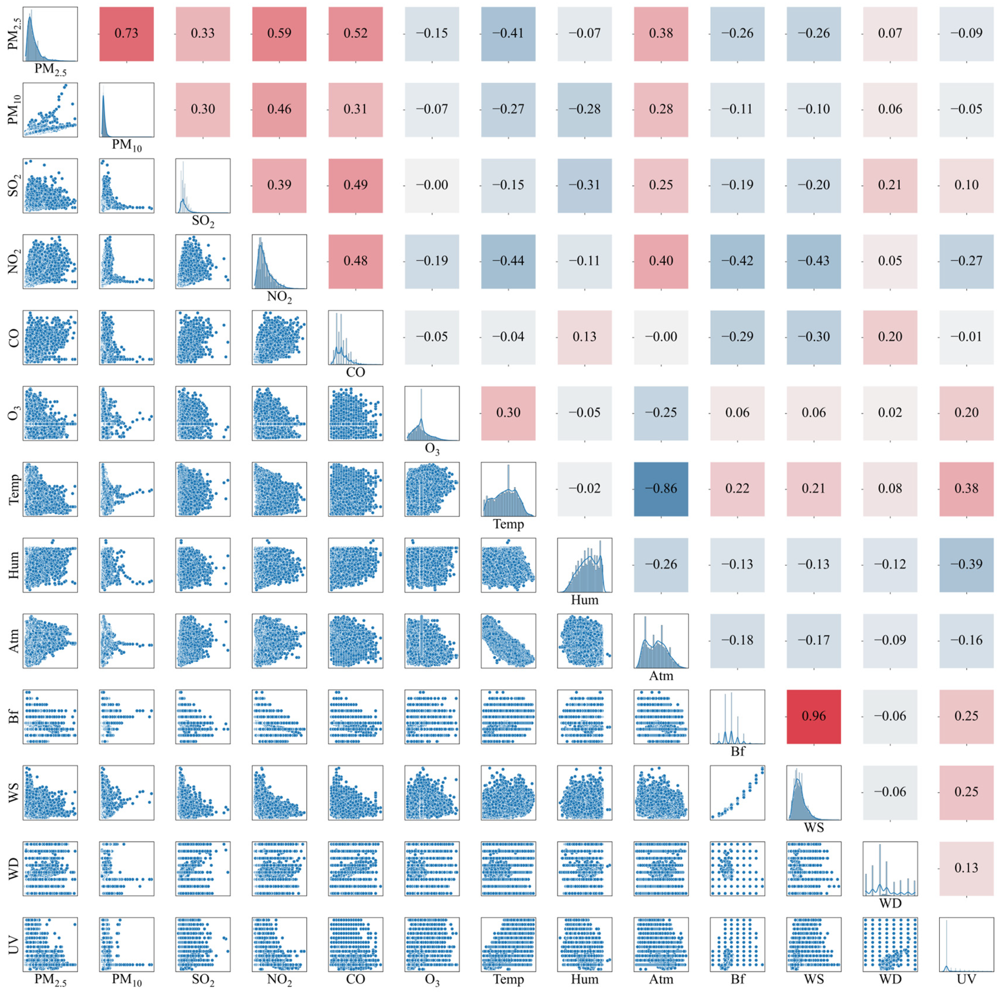
2.1.2. Correlation Analysis

The Pearson correlation coefficient, which ranges from −1 to 1, is used to analyze the relationship between variables [33]. A larger absolute value indicates a stronger correlation between variables, while a smaller absolute value suggests a weaker correlation. Other pollutants and meteorological factors may affect PM_2.5, and some correlations likely exist between these factors. Therefore, it is important to build prediction models using factors that are strongly correlated with PM_2.5 to enhance accuracy. Figure 1 presents the correlation analysis heatmap, showing that the correlation coefficients between PM_2.5 and other pollutants—PM₁₀, NO₂, CO, and SO₂—are 0.73, 0.59, 0.52, and 0.33, respectively. The correlation coefficients with PM₁₀, NO₂, and CO are above 0.5, indicating strong correlations, while the correlation with SO₂ is moderate, and that with O₃ is weak. Meteorological factors such as wind speed, direction, and temperature also show correlations with PM_2.5, influencing the results.

2.2. Feature Selection

Redundant or irrelevant features can introduce noise, potentially affecting prediction accuracy. To minimize unnecessary features and reduce model complexity, this section first determines the optimal number of features using Recursive Feature Elimination with Cross-Validation (RFECV) [34] and then selects features based on the correlation analysis. In this process, RFECV employs Support Vector Regression (SVR) as the estimator, using 10-fold cross-validation to rank and identify the optimal feature set. Mean Squared Error (MSE) is adopted as the scoring metric in this step to align with the loss functions used in our primary predictive models. While alternative metrics such as Mean Absolute Error (MAE) and Median Absolute Error (MedAE) are more robust to outliers and widely used in air pollution studies, MSE is more sensitive to large deviations, making it well-suited for identifying extreme pollution events. This heightened sensitivity to large deviations aligns closely with the priorities of environmental monitoring systems, where timely and accurate detection of extreme pollution events is critical for effective risk mitigation and protection of public health. Figure 2 shows the results from the feature selection process.

As shown in the figure, as the number of features increases, the model’s MSE gradually decreases, indicating that the initial feature selection significantly improves the model’s performance. However, when the number of features exceeds six, the MSE score tends to stabilize. Further increasing the number of features does not bring significant performance improvements and may instead increase model complexity, leading to issues such as low computational efficiency and overfitting. Therefore, based on the correlation coefficient, this paper selects six features as the optimal number; the selected variables are shown in

Table 2. Feature selection results.

Selected Variables	Correlation Coefficient
PM10	0.73
NO2	0.59
CO	0.52
Vis	−0.48
Temp	−0.41
Atm	0.38

.

2.3. Model Evaluation Metrics

To reflect the predictive performance of the proposed model, this paper chooses four evaluation metrics––MedAE, MAE, mean absolute percentage error (MAPE), and root mean squared error (RMSE)––to assess model performance. The formulas for each evaluation metric are given below.

$$\mathrm{MedAE}=\left(\left|y_1-{\widehat{y}}_1\right|,\dots ,\left|y_n-{\widehat{y}}_n\right|\right)$$

(2)

$$\mathrm{MAE}={\displaystyle \frac{{\displaystyle \sum _{i=1}^n\left|y_i-{\widehat{y}}_i\right|}}{n}}$$

(3)

$$\mathrm{MAPE}={\displaystyle \frac{100}{n}}{\displaystyle \sum _{i=1}^n\left|\frac{y_i-{\widehat{y}}_i}{y_i}\right|}$$

(4)

$$\mathrm{RMSE}=\sqrt{{\displaystyle \frac{1}{n}}{\displaystyle \sum _{i=1}^n{\left(y_i-y_i\right)}^2}}$$

(5)

In the equation, $y_i$ represents the true value, ${\widehat{y}}_i$ represents the model’s predicted value, and n represents the number of tests. The range of MedAE values is [0, ∞), while MAE, MAPE, and RMSE take values within [0, 1]. A value closer to 0 indicates smaller prediction error and higher prediction accuracy.

2.4. BiTCN

TCN is an enhanced network structure derived from CNN, incorporating causal and dilated convolution mechanisms, which are particularly effective for processing time series data [35]. Causal convolution is a key feature of TCN. It is a unidirectional, time-constrained model that preserves the causality of the input time series. This structure avoids using future time data while expanding the receptive field, making it more effective at extracting temporal features than traditional CNN [36]. If the input sequence consists of s elements, the output after causal dilated convolution is given by Equation (6).

$$F\left(s\right)=(x\ast f)\left(s\right)=\sum _{k=0}^{p-1}f\left(k\right)·x_{s-d·k}$$

(6)

where F is the causal dilated expression; x is the input sequence; f and f(k) represent the filter; s is the time step position in the current sequence where the output is calculated; * denotes the convolution operation; p is the convolution kernel size; and d is the dilation factor.

However, traditional TCN performs feature extraction in only one direction, neglecting extraction of hidden backward feature information. The nonlinear and complex nature of PM_2.5 concentration time series data may harbor important hidden backward features. To address this, this paper employs BiTCN, which extracts both forward and backward features from the PM_2.5 time series, thereby enhancing feature capture and improving the model’s overall prediction accuracy.

2.5. BiLSTM

Recurrent Neural Networks (RNNs) share parameters when processing sequential data, causing the gradients to diminish progressively during the backpropagation process, leading to the vanishing gradient problem. To address this problem, Jürgen Schmidhuber proposed the concept of LSTM for the first time in 1997 [37]. BiLSTM is an optimized neural network based on LSTM. A conventional LSTM directly inputs data features to produce the predicted output, while BiLSTM sets up two independent LSTM layers. It first feeds the information forward to obtain a set of forward results, then inputs the information backward into another LSTM module, and finally combines the forward and backward outputs to produce the final prediction [38].

2.6. QMEWOA

2.6.1. Traditional WOA

Humpback whales are naturally social creatures that live in groups. In the hunting process, the whale group surrounds the prey, then gradually reduces the encirclement by spiraling upward and releasing bubbles until the hunt succeeds. Drawing inspiration from this behavior, Mirjalili and Lewis [39] developed the WOA. WOA divides the optimization process into three stages: encirclement and contraction, bubble-net hunting, and prey searching. The combination of these behaviors enables WOA to effectively perform global and local searches in a vast solution space, gradually approaching the optimal solution to the problem.

2.6.2. Multi-Strategy Enhanced WOA Integrated with Quantum Computing

Although WOA is known for fast convergence and strong optimization capabilities, it has several limitations: (i) low diversity in the whale population, which makes it prone to local optima; (ii) a slow convergence rate in later iterations due to the spiral update strategy, making it difficult to balance exploration and exploitation; (iii) the separation of whale individuals is based solely on random probability, which can result in the loss of high-quality individuals. In conclusion, this paper presents the QMEWOA algorithm, which applies multiple strategic improvements to WOA. These improvements are detailed below.

(1)

Bernoulli chaotic mapping: Chaotic mapping generates sequences with greater ergodicity and randomness than regular random sequences, fostering a more diverse population [40]. Effective population initialization accelerates convergence and enhances the algorithm’s performance. Common chaotic mappings for population initialization include Tent, Cubic, and Bernoulli chaotic mappings. Of these, Bernoulli chaotic mapping yields a more uniform population distribution, improving diversity to some extent [41]. This paper thus adopts Bernoulli chaotic mapping to enhance population initialization, increase diversity, and improve WOA’s local search capabilities. The equation for Bernoulli chaotic mapping is

$$Z_{k+1}=\{\begin{array}{ccc}{Z}_k/(1-\mathit{\beta })& ,& 0<Z_k\le 1-\mathit{\beta }\\ (Z_k-1+\mathit{\beta })/\mathit{\beta }& ,& 1-\mathit{\beta }<Z_k<1\end{array}$$

(7)

where Z_k denotes the chaotic sequence value generated for the k-th generation, and β is the control parameter. Based on extensive experimental comparisons, Z₀ is set to 0.326, and β is set to 0.563, which yields better results in this paper.

(2)

Improved nonlinear convergence factor and time-varying weight: In WOA, the convergence factor decreases linearly from 2 to 0, but this linear decay update mechanism restricts the individual search capacity, preventing the full manifestation of WOA’s search mechanism. To better balance the global and local search mechanisms, this paper improves a by proposing a nonlinear decay strategy, with its mathematical expression given in Equation (8).

$$a=c_1\cdot \arcsin {\left(1-{\displaystyle \frac{t}{T_{\max }}}\right)}^{e^{c_2\cdot {\displaystyle \frac{t}{T_{\max }}}}}$$

(8)

where c₁ and c₂ are adjustment coefficients used to control the amplitude and decay rate of the convergence factor a. The amplitude and decay rate of a increase as the adjustment coefficients increase. Through extensive experimental analysis, c₁ and c₂ are determined to be 1.26 and 2.86, respectively. Figure 3 shows the comparison between the improved a and the traditional a. As seen in the figure, in the early iterations, a decreases gradually and slightly, expanding the global search space. In the later iterations, smaller a values help improve algorithm precision and accelerate exploitation.

To further enhance the global and local search capabilities of WOA, this paper is inspired by the feedback factor in the Slime Mold Algorithm (SMA) and proposes a feedback time-varying weight for the cooperative convergence factor a. In traditional SMA, the feedback factor V_c is constrained by the parameter c, which decreases linearly and limits local exploitation during the development phase. To address this, this paper modifies c, with the updated version defined in Equation (10):

$$V_c=2\cdot c\cdot r-c$$

(9)

$$c={\left(c_{\max }-{\displaystyle \frac{t\left(c_{\max }-c_{\min }\right)}{T_{\max }}}\right)}^k$$

(10)

where c_max and c_min are set to 1 and 0, respectively, according to the traditional SMA, while k is a tuning parameter. In this paper, the values of k are taken as 2, 4, 6, and 8, with the corresponding results shown in Figure 4a. If k is too small, the algorithm will exhibit large oscillations in the early iterations, disrupting the balance between exploration and exploitation. Conversely, if k is too large, the small oscillations in the early iterations may cause the algorithm to get stuck in a local minimum. Based on experimental verification, k is set to 6, with the resulting improvements in c and the V_c oscillation curve shown in Figure 4b. The equation for the time-varying weight of the feedback factor is given in Equation (11).

$$w=\{\begin{array}{ccc}{V}_c·{[1+e^{(𝜋·\frac{t}{T_{\max }})}]}^{V_c}& ,& t<\frac{T_{\max }}{2}\\ V_c·{[1-e^{(𝜋·\frac{t}{T_{\max }})}+\cos (𝜋·\frac{t}{T_{\max }})]}^{V_c}& ,& t\ge \frac{T_{\max }}{2}\end{array}$$

(11)

(3)

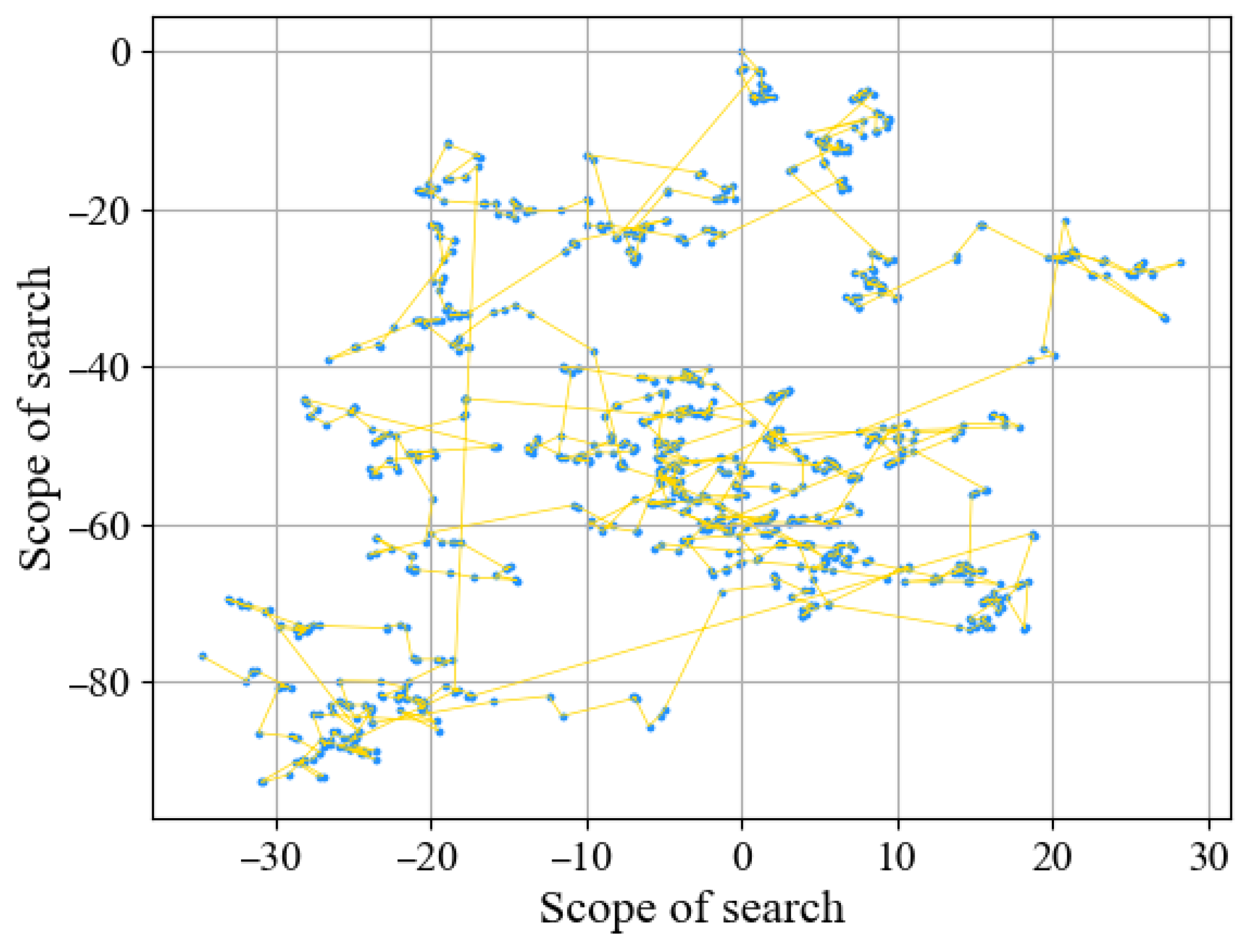
Dual-strategy improvement in the bubble net hunting phase: In the later iterations of traditional WOA, the whale individuals are more concentrated, which makes the algorithm prone to getting stuck in local optima, resulting in stagnation or premature convergence. The inertia factor in Particle Swarm Optimization (PSO) helps guide a population’s individuals toward optimization. This paper combines the PSO inertia factor with the Levy flight mechanism and mutation differential operator to create dual-strategy improvement in the shrinking encirclement phase. Levy flight, proposed by Mantegna and Topics [42], is a random walk mechanism based on the Levy distribution. It effectively improves the algorithm’s ability to avoid local optima and enhances its global search capability. In this study, the step size for the Levy flight is set to 1000 for the simulation experiments, with the results displayed in Figure 5.

As shown in the figure, the Levy flight mechanism is characterized by small-step walking and a broad search range, which aids WOA in escaping local optima and improving its global search ability. The updated position formula after introducing the Levy flight mechanism is given in Equation (12); while the spiral update position after introducing the mutation differential operator strategy is shown in Equation (13).

$$X_i\left(t+1\right)=X_i\left(t\right)+vb\cdot L\left(\gamma \right)\cdot \left(W\cdot X_A\left(t\right)-X_{best}\left(t\right)\right)$$

(12)

$$X_i\left(t+1\right)=w\cdot D^{\prime }\cdot b\cdot e^{bl}\cdot \cos \left(2\pi l\right)+X_{best}\left(t\right)+\mu$$

(13)

$$\mu =U\cdot \left(X_{best}\left(t\right)-X_i\left(t\right)\right)$$

(14)

where D′ denotes the distance between a whale individual and the current best individual, b is a constant (default value 1), l is a random number uniformly distributed in the range [−1, 1], X_best indicates the position of the current best whale, L is the Levy flight operator, γ is the step size, μ is the mutation differential factor, and U is the disturbance coefficient, which is set to 0.62 in this paper.

(4)

The sparrow follower position update method integrated with quantum particle swarm for solution generation: The position update rule for sparrow followers is that, when their fitness is low, they move to other areas to forage; otherwise, they forage near the optimal individual. The search units converge either by teleporting to the neighborhood of the optimal solution or by moving closer to the origin. However, this method lacks local search capability, making it susceptible to local optima. The Quantum Particle Swarm Optimization (QPSO) algorithm, introduced by Sun, et al. [43], simulates the uncertainty of quantum superposition states. This enables the algorithm to cover the entire search space and enhance global search capability through an adaptive potential field. Therefore, this paper combines QPSO-generated solutions with the follower update method to propose a follower position update strategy that integrates quantum computing. The position update expression after applying this strategy is shown below.

$$X_i\left(t+1\right)=\left\{\begin{array}{ccc}{P}_i\left(t\right)+Q\cdot {\mathrm{e}}^{\left({\displaystyle \frac{X_{worst}\left(t\right)-X_i\left(t\right)}{i^2}}\right)}+0.53\cdot {\phi }_i\left(t\right)\cdot \log \left({\displaystyle \frac{1}{g}}\right)\hfill & ,\hfill & i>{\displaystyle \frac{n}{2}}\hfill \\ X_p\left(t+1\right)+\left|X\left(t\right)-X_p\left(t+1\right)\right|\cdot A^{+}\cdot {\phi }_i\left(t\right)\hfill & ,\hfill & i\le {\displaystyle \frac{n}{2}}\hfill \end{array}\right.$$

(15)

$$P_i\left(t\right)=g\cdot P_i\left(t\right)+\left(1-g\right)\cdot X_{best}\left(t\right)$$

(16)

$${\phi }_i\left(t\right)=2\cdot a_t\cdot \left|C_t-X_i\left(t\right)\right|$$

(17)

$$a_t=a_0+\left(a_1-a_0\right)\cdot {\displaystyle \frac{\left(T_{\max }-t\right)}{T}}$$

(18)

Here, P_i(t) is the initial position, Q is a random number following a normal distribution, X_worst(t) is the position occupied by the worst individual in the current iteration, φ_i(t) represents the distance between the current position and the individual’s average optimal position, g is a random number following a uniform distribution, a₁ and a₀ are the contraction and expansion factors, and A is a matrix with elements of 1 or −1, and A⁺ = A^T(AA^T)⁻¹.

(5)

Quantum rotation gate update strategy: The quantum rotation gate is a crucial operation for population updating in Quantum Genetic Algorithms (QGAs), allowing the search algorithm to move closer to the optimal solution [44]. The goal of the quantum rotation gate is to converge the quantum bit probability amplitude of each quantum state gene position in the chromosome of the genetic algorithm to 0 or 1 [45]. In this paper, the quantum rotation gate is used to update the positions of individual whales. The quantum position of the k-th whale is represented by Equation (19), and the quantum rotation gate expression for the i-th whale corresponding to the j-th quantum rotation angle is shown in Equation (20).

$$\left|X_i,\left(t\right)\right.〉=\left[X_{i1}\left(t\right),X_{i2}\left(t\right),\dots ,X_{iK}\left(t\right)\right]=\left[\begin{array}{c}{\alpha }_{i1}\left(t\right),{\alpha }_{i2}\left(t\right),\dots ,{\alpha }_{iK}\left(t\right)\\ {\beta }_{i1}\left(t\right),{\beta }_{i2}\left(t\right),\dots ,{\beta }_{iK}\left(t\right)\end{array}\right]$$

(19)

$$U\left({\theta }_i\left(t+1\right)\right)=\left[\begin{array}{cc}\cos \left({\theta }_i\left(t+1\right)\right)& -\sin \left({\theta }_i\left(t+1\right)\right)\\ \sin \left({\theta }_i\left(t+1\right)\right)& \cos \left({\theta }_i\left(t+1\right)\right)\end{array}\right]$$

(20)

where ${\left|{\alpha }_{ij}\right|}^2+{\left|{\beta }_{ij}\right|}^2=1(j=1,2,\dots ,K)$, and both ${\alpha }_{ij}$ and ${\beta }_{ij}$ are real numbers, with $0\le {\alpha }_{ij}\le 1$ and $0\le {\beta }_{ij}\le 1$. The quantum rotation gate update process is as follows:

$$X_{t+1}=\left|U\left({\theta }_i\left(t+1\right)\right)\cdot X_i\left(t\right)\right|=\left|\left[\begin{array}{cc}\cos {\theta }_i\left(t+1\right)& -\sin {\theta }_i\left(t+1\right)\\ \sin {\theta }_i\left(t+1\right)& \cos {\theta }_i\left(t+1\right)\end{array}\right]\cdot X_i\left(t\right)\right|$$

(21)

2.6.3. QMEWOA Algorithm Steps

To clearly illustrate the execution process of the proposed QMEWOA algorithm, this section outlines its core steps. QMEWOA incorporates quantum rotation crossover, nonlinear dynamic weights, a cosine–sine disturbance mechanism, and a hybrid Gaussian–Cauchy mutation strategy to improve global search capability and convergence precision. The complete procedure is detailed in Algorithm 1.

Algorithm 1: QMEWOA

Input: Population size pop, dimension dim, lower bound lb, upper bound ub, maximum iteration MaxIter, fitness function fun

Output: Best fitness value GbestScore, best solution GbestPosition, convergence curve Curve

1: Initialize whale population X within bounds [lb, ub] 2: Evaluate fitness of each whale using fun() 3: Sort the population X based on fitness 4: Set GbestScore ← best fitness, GbestPosition ← corresponding whale 5: for t ← 1 to MaxIter do 6:   Set Leader ← best whale in population 7:   Compute parameters: a ← (1.26 * arcsin(1 − t/MaxIter)) ^ exp(2.86 * t/MaxIter) a2 ← −1 + t * (−1/MaxIter) vc ← 2 * exp((1 − t/MaxIter − 1))^6 * rand() − exp((1 − t/MaxIter − 1))^6 Update inertia weight w based on vc and current iteration t 8:   for i ← 1 to pop do 9:     for j ← 1 to dim do 10:       Generate random numbers r1, r2, p 11:       Compute coefficients A, C, b, l 12:       if p < 0.5 then 13:         if |A| ≥ 1 then 14:           Select random whale X_rand 15:           Compute distance D_X_rand and update X[i,j] using Lévy flight with weight w 16:         else 17:           Compute distance D_Leader 18:            Update X[i,:] using cosine–sine adaptive strategy with weight w 19:       else 20:        Select random whale X[Rindex] 21:        Compute distance2Leader and Lambda 22:        Update X[i,j] based on WOA prey behavior with weight w 23:   end for 24:   Update joiners via LJDUpdate 25:   Apply boundary control on X 26:   Evaluate fitness of updated X 27:   Perform quantum rotation crossover with GbestPosition 28:   Sort population and update Gbest if improved 29:   for i ← 1 to pop do 30:     Apply DE-inspired update strategy on X[i] with parameters fhai, wmega 31:     Perform boundary control and evaluate fTemp 32:     if fTemp < GbestScore then 33:      Update GbestScore and GbestPosition 34:   end for 35:   Apply Gaussian-Cauchy mutation on GbestPosition 36:   if mutated fitness < GbestScore then 37:     Update GbestScore and GbestPosition 38:   Record Curve[t] ← GbestScore 39:   Print iteration info 40: end for 41: return GbestScore, GbestPosition, Curve

2.7. QCAM

The traditional attention mechanism computes the attention distribution across all time-step features. In contrast, the CAM maintains the causal relationships in temporal or sequential data, avoiding future information leakage during training and enhancing model credibility [46]. Inspired by the ability of Quantum State Mapping (QSM) to obtain higher-dimensional feature information and improve the performance of the attention mechanism [47], this paper improves CAM and proposes a QCAM.

2.7.1. QSM

QSM refers to a mathematical mapping strategy inspired by the wave function that describes a microscopic particle system. The wave function is a fundamental concept in quantum mechanics, representing the probability amplitude of a particle at a specific point in space and time. In the context of a one-dimensional particle confined in an infinitely deep square potential well, the wave function takes a simple form, and the transient Schrödinger equation can be explicitly solved. The transient Schrödinger equation is given by Equation (22).

$$\left\{\begin{array}{l}\Psi \left(x,t\right)={\displaystyle \sum _{n=1}^{\infty }{c}_n\sqrt{\frac{2}{a}}\sin \left(\frac{n\pi }{a}x\right)e^{-i{E}_{n}t/\hslash }}\hfill \\ E_n={\displaystyle \frac{n^2{\pi }^2{\hslash }^2}{2m{a}^2}}\hfill \end{array}\right.$$

(22)

where a is the well width, m is the quantum mass, taken as 1 in this paper, and $\hslash$ denotes Planck’s constant, set to 6.62 in this paper. Assuming the pooled feature vector is $X\in {ℝ}^{1\times d}$, associating the particle state with the feature vector gives QSM: $X\to {\left|\Psi \left(X\right)\right|}^2 \left({\left|\Psi \left(X\right)\right|}^2\in \left[0,1\right]\right)$. This maps the feature vectors from the original space to the probability space, enabling the neural network to leverage the global information probability distribution to produce more effective attention [48]. Its expression is given by Equation (23).

$${\left|\Psi \left(X\right)\right|}^2={\displaystyle \frac{2}{a}}{\displaystyle \sum _{n=1}^{\infty }{c}_n^2\cdot {\sin }^2\left(\frac{n\pi }{a}x\right)}$$

(23)

2.7.2. CAM Integrated with QSM

QCAM first integrates the input features into attention distributions at different time steps, concatenates them into a T × T attention matrix, and then maps the matrix to a high-dimensional probability space using quantum-inspired QSM mapping. The QSM-mapped features are then concatenated, and a mask is generated by filling the upper triangle of the attention matrix with negative infinity, ensuring that the upper triangular elements become zero after applying the Softmax layer. Finally, the Softmax-processed mask matrix is added to the feature matrix to produce the final output.

2.7.3. QCAM Algorithm Steps

To clarify the workflow of the proposed QCAM, this section presents its key computational steps. QCAM integrates frequency-domain representations, channel-wise attention modeling, and a QSM to effectively capture complex temporal dependencies under causality constraints. The detailed procedure is outlined in Algorithm 2.

Algorithm 2: QCAM

Input: Input tensor inputs ∈ ℝ^(B × L × D)

Output: Attention-enhanced feature representation

1: Initialize two Conv1D layers with 64 filters and kernel size 1 (Conv1, Conv2) 2: function QSM_Mapping(attention_scores) 3:   Set constants: a ← 1.0, m ← 1.0, ℏ ← 1.0 4:   Define sequence length n ← [1, 2,..., L] 5:   Compute energy levels En ← (n2 * π2 * ℏ2)/(2ma2) 6:   Compute spatial grid x ← linspace(0, a, L), time t ← 1.0 7:   for each n_i in n do 8:     Compute ψn(x, t) ← √(2/a) * sin(n_i * π * x/a) * cos(En * t/ℏ) 9:   end for 10:   Aggregate ψ ← ∑ ψn(x, t) 11:   Compute probability density ψ2 ← |ψ|2 12:   Tile ψ2 across batch dimension 13:   return ψ2 14: end function 15: function CALL(inputs) 16:   Compute FFT of inputs: fft ← FFT(inputs) 17:   Extract frequency features: freq_features ← concat(Re(fft), Im(fft)) 18:   Compute average pooled features: avg_pool ← mean(freq_features, axis = 1) 19:   Compute max pooled features: max_pool ← max(freq_features, axis = 1) 20:   avg_out ← Conv2(Conv1(avg_pool)) 21:   max_out ← Conv2(Conv1(max_pool)) 22:   Compute channel attention: channel_attn ← avg_out + max_out 23:   Compute raw attention scores: scores ← channel_attn · channel_attnᵀ 24:   Apply QSM mapping: qsm_scores ← QSM_Mapping(scores) 25:   Create lower triangular mask M ∈ ℝ^(L × L) 26:   Apply causal masking: masked_scores ← qsm_scores ⊙ M + (1 − M) * −∞ 27:   Normalize attention weights: α ← softmax(masked_scores, axis = −1) 28:   Compute weighted output: output ← α · freq_features 29:   return output 30: end function

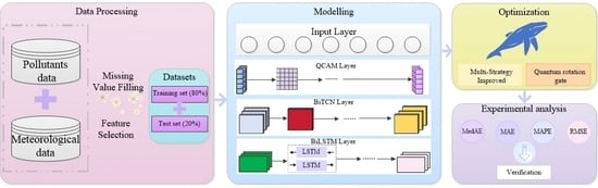
2.8. Modeling Process

The modeling steps of the proposed method are shown in Figure 6, with the specific steps outlined as follows:

(1)

Missing values in the air quality and meteorological time series datasets are first filled. Then, feature variables are selected using correlation coefficients and RFECV to reduce model complexity.

(2)

The dataset is split into training and testing sets with an 8:2 ratio. The input data is first assigned attention weights through QCAM, then feature extraction is performed by BiTCN, and finally, predictions are made using BiLSTM.

(3)

QMEWOA is employed to optimize the model’s hyperparameters. Initially, the whale population size, iteration count, and other algorithm parameters are set. QMEWOA iteratively updates the fitness values, ultimately identifying the optimal hyperparameters. These optimal hyperparameters are then applied to the QCAM-BiTCN-BiLSTM model to obtain the locally optimal model using the best features.

(4)

Finally, the performance of the proposed model is compared with other models to validate its superiority.

3. Experiments and Analysis

3.1. Experimental Environment

The experiments were carried out on a computer running Windows 11, with a 12th Gen Intel(R) Core(TM) i5-12600KF processor, an NVIDIA Geforce 4060 Ti 16 GB graphics card, and 32 GB of RAM, using Python 3.9.18. The neural network is built using the Keras library (version 2.8.0); data processing is performed using libraries such as Numpy (version 1.22.4) and Pandas (version 1.2.4); and visualization is implemented with the Matplotlib library (version 3.5.1).

3.2. Comparative Analysis of Optimization Algorithm Performance

To comprehensively evaluate the optimization performance of QMEWOA, ten classical benchmark functions were selected. These functions are widely used in the literature to assess the effectiveness of nature-inspired metaheuristic algorithms [49,50]. Additionally, QMEWOA is compared with WOA, the improved whale optimization algorithm (IWOA) [51], the grey wolf optimization algorithm (GWO), PSO, and the dung beetle optimization (DBO) algorithm.

Table 3. Test function basic information.

Function Expression	Dimension	Range	Optimum
$F_1={\displaystyle \sum _{i=1}^n{x}_i^2}$	30	[−100, 100]	0
$F_2={\displaystyle \sum _{i=1}^n\left|x_i\right|}+{\displaystyle \prod _{i=1}^n\left|x_i\right|}$	30	[−100, 100]	0
$F_3={\displaystyle \sum _{i=1}^n{\left({\displaystyle \sum _{j=1}^n{x}_i}\right)}^2}$	30	[−100, 100]	0
$F_4=\max \left\{\left|x_i\right|,1\le i\le n\right\}$	100	[−100, 100]	0
$F_5={\displaystyle \sum _{i=1}^n\left[100\left(x_{i+1}-x_i^2\right)+{\left(x_i-1\right)}^2\right]}$	30	[−30, 30]	0
$F_6={\displaystyle \sum _{i=1}^n{\left(\left[x_i+0.5\right]\right)}^2}$	30	[−100, 100]	0
$F_7=-20e^{\left(-0.2\sqrt{{\displaystyle \frac{1}{n}}{x}_i^2}\right)}-e^{\left({\displaystyle \frac{1}{n}}{\displaystyle \sum _{i=1}^n\cos \left(2\pi x_i\right)}\right)}+20+e$	30	[−32, 32]	0
$F_8={\displaystyle \sum _{i=1}^n\left[x_i^2-10\cos \left(2\pi x_i+10\right)\right]}$	30	[−5.12, 5.12]	0
$F_9={\displaystyle \frac{1}{4000}}{\displaystyle \sum _{i=1}^n{x}_i^2}-{\displaystyle \prod _{i=1}^n\cos \left(\frac{x_i}{\sqrt{i}}\right)+1}$	30	[−600, 600]	0
$F_{10}={\left({\displaystyle \frac{1}{500}}+{\displaystyle \sum _{j=1}^{25}\frac{1}{j+{\displaystyle \sum _{i=1}^2{\left(x_i-a_{ij}\right)}^6}}}\right)}^{-1}$	2	[−65, 65]	1

shows the basic information of the test functions. F₁ to F₆ are unimodal test functions used to evaluate the algorithm’s local exploitation ability, while F₇ to F₁₀ are multimodal test functions used to assess the algorithm’s global exploration ability. Dimensions F1 to F9 are set to 30, and F10 is a fixed-dimension multimodal test function with a dimension of 2. The theoretical optimal values for F1 to F9 are 0, and for F10, it is 1. To ensure fairness, all algorithms are set with a population size of 30, and the experiments are conducted for 500 iterations.

To eliminate randomness in the results, each algorithm is run independently 50 times, and its optimal value, mean, and standard deviation are calculated. The optimal value reflects the solution’s quality, the mean represents its accuracy, and the standard deviation indicates its stability.

Table 4. Test function comparison results.

Algorithms	Metric	F1	F2	F3	F4	F5	F6	F7	F8	F9	F10
QMEWOA	Best	0	5.33 × 10−216	0	3.192 × 10−264	6.546 × 10−7	1.553 × 10−10	4.440 × 10−16	0	0	0.998
	Avg	0	8.40 × 10−127	9.101 × 10−296	4.642 × 10−132	16.100	0.135	4.440 × 10−16	0	0	1.946
	Std	0	4.14 × 10−126	0	3.249 × 10−131	14.231	0.938	0	0	0	2.429
WOA	Best	2.047 × 10−24	7.117 × 10−16	2.873 × 10−6	1.636 × 10−6	26.284	0.529	3.00 × 10−6	0	0	0.998
	Avg	1.191 × 10−20	2.219 × 10−14	0.005	0.000	27.672	1.584	3.410 × 10−15	4.662 × 10−17	0	1.528
	Std	6.362 × 10−20	4.265 × 10−14	0.016	0.000	0.685	0.587	1.349 × 10−14	2.674 × 10−16	0	0.734
IWOA	Best	3.307 × 10−47	5.915 × 10−28	1.164 × 10−17	6.409 × 10−14	26.228	1.418	4.440 × 10−16	0	0	0.998
	Avg	2.245 × 10−37	1.828 × 10−24	5.828 × 10−12	1.086 × 10−10	27.806	2.932	4.423 × 10−15	0	0	3.716
	Std	1.089 × 10−36	4.234 × 10−24	2.135 × 10−11	2.416 × 10−10	0.755	0.566	1.355 × 10−15	0	0	3.044
GWO	Best	1.668 × 10−29	1.702 × 10−17	1.009 × 10−8	8.542 × 10−8	26.025	5.365 × 10−5	7.505 × 10−14	5.684 × 10−14	0	0.99
	Avg	1.401 × 10−27	1.119 × 10−16	8.846 × 10−6	7.305 × 10−7	27.326	0.767	1.058 × 10−13	2.338	0.004	3.801
	Std	1.737 × 10−27	1.514 × 10−16	2.050 × 10−5	8.489 × 10−7	0.716	0.367	1.871 × 10−14	3.293	0.110	3.785
PSO	Best	229.904	289.187	3383.222	18.858	11,577.624	211.511	5.933	79.564	1.387	0.998
	Avg	1430.455	692.692	13,778.357	31.1195	397,781.152	1883.327	11.965	126.838	15.388	2.164
	Std	1011.679	179.456	6226.064	5.590	489,303.742	2021.789	2.739	25.149	10.493	1.727
DBO	Best	2.957 × 10−58	1.367 × 10−30	1.145 × 10−54	2.854 × 10−27	26.873	0.025	4.440 × 10−16	0	0	0.998
	Avg	4.197 × 10−26	14.801	16,049.159	1.689 × 10−24	64.023	0.117	1.653	18.511	0.000	1.629
	Std	2.867 × 10−25	18.892	15,446.437	5.491 × 10−24	189.241	0.115	4.479	24.379	0.001	1.584

Note: Bold values indicate the best performance among all compared Algorithms.

presents the experimental comparison results of QMEWOA with other algorithms, while Figure 7 shows the convergence curves for the corresponding test functions.

The following conclusions can be drawn from the above charts and tables. (a) QMEWOA significantly outperforms traditional WOA in solution quality, delivering more stable and higher-quality results across all test functions. Although both algorithms exhibit similar trends for some test functions, QMEWOA demonstrates superior convergence speed and optimization precision. (b) Benefiting from multi-strategy improvements, QMEWOA demonstrates an overall improvement in solution stability and quality compared to the single-strategy IWOA. For instance, in F1 and F3, QMEWOA finds the global optimal solution, while IWOA continues to be stuck in local optima, resulting in a large discrepancy between the two. From the convergence curves, QMEWOA shows stronger exploration and search abilities, while also ensuring solution accuracy, highlighting the effectiveness and superiority of the multi-strategy improvements in the algorithm’s performance. (c) QMEWOA consistently outperforms other algorithms, demonstrating rapid convergence towards the optimal solution for both single-peak and multi-peak test functions, while maintaining excellent exploration capabilities. This highlights QMEWOA’s superior overall performance.

3.3. Optimization Parameter Experimental Analysis

This study uses the MSE of the training set as the fitness function, with 10 iterations set for iterative optimization of the QCAM-BiTCN-BiLSTM hyperparameters. The parameters to be optimized for QMEWOA include the number of neurons (Hidden_dim), the batch size (Batch_size), and the number of iterations (Epoch). The search spaces for the hyperparameters optimized by QMEWOA were defined based on both domain knowledge and prior studies of deep neural networks for time series forecasting [52]. Specifically, the number of neurons was searched within the range [10, 512], the batch size within [1, 512], and the number of training epochs within [10, 50]. These ranges were chosen to strike a balance among model complexity, training efficiency, and generalization performance. Preliminary experiments confirmed that these intervals encompass the most performance-sensitive regions of the hyperparameter space. Figure 8 illustrates the optimization iteration process. The MSE rapidly decreases as the number of iterations increases, indicating that QMEWOA improves the model’s performance significantly in the early stages. In the later stages, the MSE stabilizes, suggesting that the model is nearing convergence. The optimal hyperparameters are 461.253, 512, and 28.92. The rapid decline of the curve indicates that the QMEWOA algorithm has high search efficiency in optimizing QCAM-BiTCN-BiLSTM.

3.4. Hyperparameter Settings

In this study, the dataset is split into training and testing sets with an 8:2 ratio. The experiment uses MAE as the loss function and the Adam optimizer for training. The TCN layer has an expansion rate of 0.2, with a convolution kernel size of 3. Detailed model parameters are listed in

Table 5. Model parameters.

Models	Neuron	Batch Size	Epoch	Learning Rate	Dropout Rate	Leaf Node	Maximum Depth	Embed Dim	Seed
XGBOOST	/	/	/	/	/	100	100	/	3407
LSTM	512	512	50	0.0003	0.2	/	/	/	3407
BiLSTM	512	512	50	0.0003	0.2	/	/	/	3407
Transformer	512	512	50	0.0003	0.2	/	/	512	3407
CAM-BiTCN-BiLSTM	512	512	50	0.0003	0.2	/	/	/	3407
xLSTM-KAN	512	512	50	0.0003	0.2	/	/	512	3407
QMEWOA-QCAM-BiTCN-BiLSTM	[10–512]	[1–512]	[10–50]	0.0003	0.2	/	/	/	3407

Note: “/” indicates that the parameter is not applicable or not used for the corresponding model.

.

3.5. Experimental Results Analysis

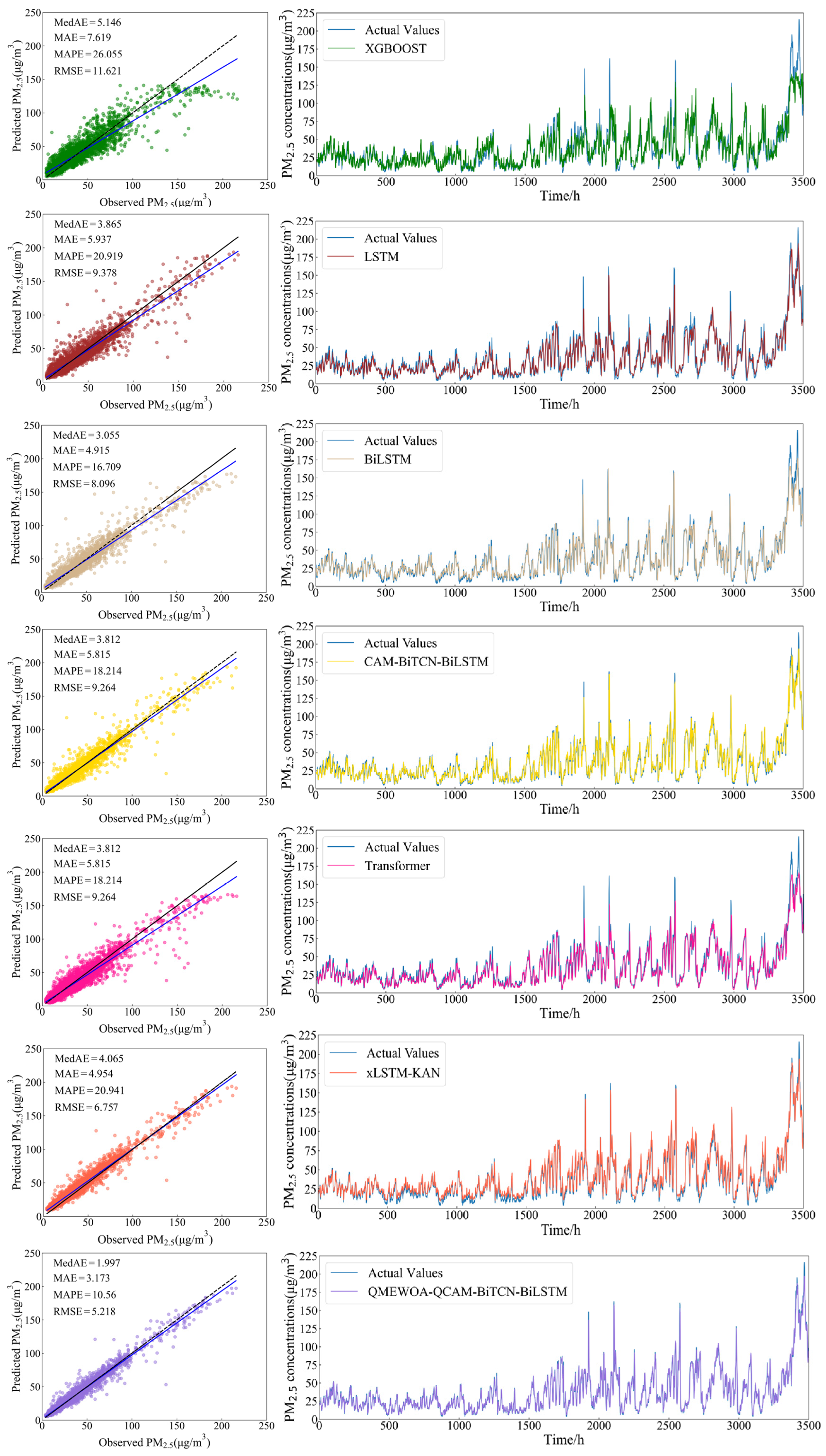
3.5.1. Comparison Experiment

To validate the performance of the proposed model, four evaluation metrics—MedAE, MAE, MAPE, and RMSE—were calculated and compared with the other six models listed in the table above. The prediction evaluation results are presented in

Table 6. Model evaluation results.

Models	MedAE	MAE	MAPE/%	RMSE
XGBOOST	5.146	7.619	26.055	11.621
LSTM	3.865	5.937	20.919	9.378
BiLSTM	3.055	4.915	16.709	8.096
Transformer	3.812	5.815	18.214	9.264
CAM-BiTCN-BiLSTM	2.733	4.410	14.829	7.344
xLSTM-KAN	4.065	4.954	20.941	6.757
QMEWOA-QCAM-BiTCN-BiLSTM	1.997	3.173	10.560	5.218

Note: Bold values indicate the best performance among all compared models.

, and the prediction trend curves are shown in Figure 9.

As shown in Figure 9, QMEWOA-QCAM-BiTCN-BiLSTM outperforms six comparison models on the test set. The proposed model accurately predicts future PM_2.5 trends and identifies turning points and significant shifts in the overall trend. It also captures the complex fluctuations of PM_2.5 concentrations over time. In addition, the PM_2.5 concentration time series may exhibit multiple sudden extreme values, potentially influenced by short-term pollution events or extreme weather conditions, making the prediction task more complex and challenging. Traditional models often fail to capture the nonlinear characteristics and sudden changes in PM_2.5 concentrations, limiting their predictive performance. In contrast, QMEWOA-QCAM-BiTCN-BiLSTM optimizes hyperparameters via QMEWOA, improving prediction robustness. The integration of QCAM enhances the model’s ability to capture key features, ensuring high accuracy even during rapid changes and fluctuations. Moreover, the collaboration between BiTCN and BiLSTM enables the model to effectively capture temporal dependencies and local feature relationships, leading to more accurate future PM_2.5 predictions.

Comparison of the multi-metric evaluation results for PM_2.5 concentration prediction in Table 6 reveals that the proposed model demonstrates superior predictive performance over XGBOOST, LSTM, BiLSTM, Transformer, CAM-BiTCN-BiLSTM, and xLSTM-KAN. In contrast to traditional single models, although these models excel in addressing certain nonlinear relationships and high-dimensional data, their performance is constrained when dealing with more complex PM_2.5 concentration time series. The proposed model, enhanced by its feature extraction module and optimization strategies, captures and predicts PM_2.5 concentration time series more effectively. Compared to XGBOOST, the model achieves a 61.2% reduction in MedAE and decreases MAPE and RMSE by 15.5% and 55.10%, respectively. Compared to LSTM, it reduces MAE, MedAE, MAPE, and RMSE by 69.04%, 48.33%, 10.36%, and 44.36%, respectively. Compared to BiLSTM, it lowers these error metrics by 34.63%, 35.44%, 6.15% and 35.55%, respectively. Similarly, compared to the Transformer, the model achieves reductions of 47.61% in MedAE, 45.43% in MAE, 7.65% in MAPE, and 43.67% in RMSE. These results underscore the model’s strong predictive capabilities, particularly in handling the complex nonlinear patterns of PM_2.5 concentration time series.

Hybrid models typically leverage multiple sub-models to process different features or data layers, improving prediction accuracy but also increasing training complexity due to extensive hyperparameter tuning. The proposed model addresses this challenge by integrating QMEWOA, which automates and optimizes parameter selection, reducing the need for manual tuning while enhancing accuracy and robustness. Additionally, QCAM further strengthens the model’s ability to capture both long-term and short-term dependencies, effectively handling intricate time series patterns. Compared to CAM-BiTCN-BiLSTM, the proposed model achieves a 26.93% reduction in MedAE, with decreases of 28.05% in MAE, 4.27% in MAPE, and 28.95% in RMSE. Similarly, against xLSTM-KAN, it reduces MedAE by 50.87%, MAE by 35.95%, MAPE by 10.38%, and RMSE by 22.78%. These findings highlight the effectiveness of QMEWOA-QCAM-BiTCN-BiLSTM in capturing global dependencies and efficiently extracting features from complex nonlinear PM_2.5 concentration time series data, demonstrating a clear advantage over both single and hybrid models across all evaluation metrics.

Based on the above experimental analysis, the proposed model shows significant advantages in prediction accuracy. Compared to traditional single models, a single model’s direct prediction of nonlinear and highly complex PM_2.5 concentration time series data shows room for improvement, with relatively high prediction errors. This is primarily because single models often fail to fully capture the complex patterns and nonlinear characteristics within the PM_2.5 concentration time series, thus impacting prediction accuracy and robustness. In comparison, while hybrid models enhance prediction performance to a certain extent, they still encounter problems like a complex parameter optimization process and inefficient feature extraction. Although hybrid models combine the advantages of multiple modules to improve upon traditional single models, they still rely on tedious manual parameter tuning and feature engineering when handling complex data. Additionally, coordination between parameters of different modules may affect overall prediction performance. The proposed model significantly enhances prediction accuracy and robustness by integrating QMEWOA and QSM with BiTCN’s efficient feature extraction and parameter optimization, thereby improving its ability to predict PM_2.5 concentration variations.

To assess whether the proposed QMEWOA-QCAM-BiTCN-BiLSTM model significantly outperforms the comparison models on the test set, the differences between its prediction error sequences and those of the comparison models were computed and defined as the DM test difference sequence. Under the null hypothesis that the proposed model performs equivalently to the comparison models, six alternative models were selected for the DM statistical test. As shown in

Table 7. DM test results comparing the proposed model with other models.

Comparison Methods	QMEWOA-QCAM-BiTCN-BiLSTM
XGBOOST	−16.602 ***
LSTM	−8.785 ***
BiLSTM	−17.745 ***
Transformer	−9.009 ***
CAM-BiTCN-BiLSTM	−8.581 ***
xLSTM-KAN	−21.182 ***

Note: Sample size N = 3503; *** indicates p < 0.01.

, the DM statistics for QMEWOA-QCAM-BiTCN-BiLSTM are all significant at the 1% level, rejecting the null hypothesis and confirming the model’s superior predictive performance over the comparison models. These results further validate the model’s strong predictive accuracy and robustness.

3.5.2. Ablation Experiment

To further analyze the necessity and independent contributions of each key module in the QMEWOA-QCAM-BiTCN-BiLSTM model structure, ablation experiments are conducted by removing the optimization algorithm, QSM, and attention mechanism as variant models. The structure and prediction results of each model are presented in

Table 8. Ablation experiment results.

Model Description	Model Name	MedAE	MAE	MAPE/%	RMSE
Remove QMEWOA	QCAM-BiTCN-BiLSTM	3.109	4.239	14.334	6.479
Remove QSM	CAM-BiTCN-BiLSTM	2.733	4.410	14.829	7.344
Remove CAM	BiTCN-BiLSTM	3.098	4.779	15.858	7.637
Remove BiTCN	BiLSTM	3.055	4.860	16.709	7.990
Proposed Model	QMEWOA-QCAM-BiTCN-BiLSTM	1.997	3.173	10.560	5.218

Note: Bold values indicate the best performance among all compared models.

.

The table demonstrates that the proposed model outperforms others regarding fit and error metrics. The performance improvements are largely due to the efficient optimization provided by QMEWOA. Specifically, the model shows a 35.77% reduction in MedAE, a 25.15% decrease in MAE, and reductions of 3.77% and 19.46% in MAPE and RMSE, respectively, compared to the version without QMEWOA optimization. Benefiting from the high-dimensional feature capture capability of QSM, the proposed model reduces the other error metrics by 26.54%, 28.05%, 4.27%, and 28.95%, respectively. Compared to BiTCN-BiLSTM, the proposed model reduces the other error metrics by 35.54%, 33.61%, 5.3%, and 31.67%, respectively. The proposed model also outperforms the baseline BiLSTM model without feature extraction, reducing MedAE by 34.63%, MAE by 35.44%, MAPE by 6.15%, and RMSE by 35.55%.

Compared to the other four ablation models, the proposed model shows improvements in all evaluation metrics, further confirming the effectiveness of the innovative approach in optimizing prediction accuracy and enhancing model performance. These improvements enhance the model’s capability to process nonlinear and complex PM_2.5 concentration time series, while also boosting its adaptability and reliability in real-world prediction tasks, demonstrating its superiority.

3.5.3. Five-Dimensional Evaluation of Practical Utility

To evaluate the practical utility of the proposed model, we establish a five-dimensional assessment framework that integrates both qualitative and quantitative indicators. Specifically, the framework comprises Parameter Efficiency (P), Model Size (M), R² Performance (R), Scalability (S), and Deployability (D). Together, these dimensions provide a comprehensive evaluation that captures not only predictive accuracy and computational efficiency, but also the model’s adaptability to large-scale data and its potential for real-world deployment in air quality monitoring systems.

As illustrated in Figure 10, the proposed QMEWOA-QCAM-BiTCN-BiLSTM model achieves consistently strong results across all five dimensions. It ranks highest in R², scalability, and deployability, highlighting its predictive strength, adaptability to expanding datasets, and suitability for real-time application. Despite its complex architecture integrating multiple deep learning and optimization components, the model maintains a reasonable parameter count and compact size, confirming that its performance improvements do not come at the cost of efficiency. In comparison, traditional models like XGBOOST and BiLSTM offer compact architectures and efficient parameter usage but lag in terms of predictive accuracy, scalability, and readiness for deployment. Transformer-based models show moderate accuracy but are hindered by their computational complexity and high inference costs, limiting their practical applicability.

This comprehensive evaluation confirms that the proposed model delivers not only high predictive accuracy, but also the efficiency and practicality required for real-time deployment, making it a strong candidate for PM_2.5 monitoring in operational settings.

3.5.4. Generalization Experiment

PM_2.5 concentration time series vary significantly due to regional differences, seasonal changes, and environmental factors. Therefore, a model’s generalization capability is crucial for practical air quality forecasting. To evaluate the model’s generalization performance, this study uses air quality data from Beijing, China recorded between March 2013 and December 2016 by the China National Environmental Monitoring Center (www.cnemc.cn, accessed on 18 July 2025). A comparative experiment was conducted using the proposed modeling framework and reference models to assess generalization. The prediction performance of each model for Beijing is summarized in

Table 9. Comparative results from the generalization experiment.

Models	MedAE	MAE	MAPE/%	RMSE
XGBOOST	10.710	18.929	45.165	31.310
LSTM	16.440	22.611	75.176	31.398
BiLSTM	13.233	19.871	54.124	29.522
Transformer	15.990	18.254	88.87	25.690
CAM-BiTCN-BiLSTM	9.669	16.570	54.390	25.900
xLSTM-KAN	13.717	18.823	61.107	27.204
QMEWOA-QCAM-BiTCN-BiLSTM	5.439	10.134	26.535	18.738

Note: Bold values indicate the best performance among all compared models.

.

As shown in Table 9, the proposed QMEWOA-QCAM-BiTCN-BiLSTM model demonstrates the best generalization performance, surpassing all comparison models. On the air quality dataset of Beijing from 2013 to 2016, the model achieved a MedAE of 5.439, MAE of 10.134, MAPE of 26.535%, and RMSE of 18.738, significantly outperforming the other six comparison methods in all evaluation metrics. The model’s superior MAPE score highlights its ability to maintain high prediction accuracy across varying concentration levels, underscoring its strong generalization capability. These findings confirm that the model is applicable beyond Ma’anshan, demonstrating its potential for broader regional adaptation. The QMEWOA-QCAM-BiTCN-BiLSTM model exhibits superior generalization ability compared to other models, offering an effective solution for PM_2.5 concentration prediction.

4. Future Research Trends

Although this study employs Pearson correlation and SVR-based RFECV for feature selection, these methods focus mainly on improving predictive accuracy and offer limited interpretability. Future work will explore incorporating interpretable or domain-informed feature selection methods, such as causal inference models or expert-driven approaches, to reveal key drivers of PM_2.5 variation and support evidence-based policy development.

Moreover, despite its strong predictive performance, the proposed model lacks interpretability and explainability mechanisms, limiting transparency and obscuring how input features influence prediction outcomes. In environmental contexts, where transparency, trust, and accountability are critical, future research should integrate interpretable machine learning methods, such as SHAP or LIME. These tools can clarify how input features influence model outputs, thereby assisting policymakers in designing more effective pollution control strategies.

5. Conclusions

PM_2.5 concentration time series are highly nonlinear and complex and are influenced by various factors, making accurate prediction crucial for environmental pollution control. While traditional machine learning and deep learning models still struggle with accuracy and stability in forecasting PM_2.5 concentrations, hybrid models often face challenges related to parameter definition, leading to significant prediction errors. This paper focuses on PM_2.5 concentration time series data and proposes a QMEWOA-QCAM-BiTCN-BiLSTM prediction model, combining optimization with prediction. The model integrates quantum mapping and a masking attention mechanism to improve prediction accuracy and handle complex data patterns. The proposed model introduces innovations in parameter optimization, attention mechanisms, and feature extraction. By combining QMEWOA and QSM with BiTCN’s feature extraction framework, the model significantly enhances both prediction accuracy and robustness. The QMEWOA algorithm effectively searches for the optimal parameter combination globally, overcoming the local optimum issue of traditional WOA and improving the model’s learning efficiency. Meanwhile, by combining QSM and BiTCN’s feature extraction methods, the model can better handle complex patterns in PM_2.5 concentration time series data, especially by capturing long-term and short-term dependencies and nonlinear features, further enhancing the model’s ability to predict PM_2.5 concentration trends. The results from the comparison and ablation experiments show that the QMEWOA-QCAM-BiTCN-BiLSTM model outperforms other models in forecasting PM_2.5 concentrations. Furthermore, to assess the adaptability of the proposed model across different regions, this study conducted a generalization experiment using PM_2.5 concentration data from Beijing. The experimental results indicate that, compared to the comparison models, the proposed model exhibits superior generalization performance and demonstrates strong cross-regional predictive capability. This innovative model offers an efficient and reliable solution for predicting PM_2.5 concentrations, contributing to the advancement of intelligent air pollution monitoring and prevention strategies.

References

1. Zeng, T.; Xu, L.; Liu, Y.; Liu, R.; Luo, Y.; Xi, Y. A hybrid optimization prediction model for PM2.5 based on VMD and deep learning. Atmos. Pollut. Res. 2024, 15, 102152. [Google Scholar] [CrossRef]
2. Yu, Q.; Yuan, H.-W.; Liu, Z.-L.; Xu, G.-M. Spatial weighting EMD-LSTM based approach for short-term PM2.5 prediction research. Atmos. Pollut. Res. 2024, 15, 102256. [Google Scholar] [CrossRef]
3. Kaur, M.; Singh, D.; Jabarulla, M.Y.; Kumar, V.; Kang, J.; Lee, H.-N. Computational deep air quality prediction techniques: A systematic review. Artif. Intell. Rev. 2023, 56 (Suppl. 2), 2053–2098. [Google Scholar] [CrossRef]
4. Woody, M.; Wong, H.-W.; West, J.; Arunachalam, S. Multiscale predictions of aviation-attributable PM2.5 for U.S. airports modeled using CMAQ with plume-in-grid and an aircraft-specific 1-D emission model. Atmos. Environ. 2016, 147, 384–394. [Google Scholar] [CrossRef]
5. Mao, X.; Shen, T.; Feng, X. Prediction of hourly ground-level PM2.5 concentrations 3 days in advance using neural networks with satellite data in eastern China. Atmos. Pollut. Res. 2017, 8, 1005–1015. [Google Scholar] [CrossRef]
6. MacIntosh, D.L.; Stewart, J.H.; Myatt, T.A.; Sabato, J.E.; Flowers, G.C.; Brown, K.W.; Hlinka, D.J.; Sullivan, D.A. Use of CALPUFF for exposure assessment in a near-field, complex terrain setting. Atmos. Environ. 2010, 44, 262–270. [Google Scholar] [CrossRef]
7. Righi, S.; Lucialli, P.; Pollini, E. Statistical and diagnostic evaluation of the ADMS-Urban model compared with an urban air quality monitoring network. Atmos. Environ. 2009, 43, 3850–3857. [Google Scholar] [CrossRef]
8. Kumar, A.; Patil, R.S.; Dikshit, A.K.; Kumar, R. Application of AERMOD for short-term air quality prediction with forecasted meteorology using WRF model. Clean Technol. Environ. Policy 2017, 19, 1955–1965. [Google Scholar] [CrossRef]
9. Soni, M.; Verma, S.; Mishra, M.K.; Mall, R.; Payra, S. Estimation of particulate matter pollution using WRF-Chem during dust storm event over India. Urban Clim. 2022, 44, 16. [Google Scholar] [CrossRef]
10. Gao, J.; Tian, H.; Cheng, K.; Lu, L.; Zheng, M.; Wang, S.; Hao, J.; Wang, K.; Hua, S.; Zhu, C. The variation of chemical characteristics of PM2.5 and PM10 and formation causes during two haze pollution events in urban Beijing, China. Atmos. Environ. 2015, 107, 1–8. [Google Scholar] [CrossRef]
11. Chemel, C.; Fisher, B.; Kong, X.; Francis, X.; Sokhi, R.; Good, N.; Collins, W.; Folberth, G. Application of chemical transport model CMAQ to policy decisions regarding PM2.5 in the UK. Atmos. Environ. 2014, 82, 410–417. [Google Scholar] [CrossRef]
12. Nopmongcol, U.; Koo, B.; Tai, E.; Jung, J.; Piyachaturawat, P.; Emery, C.; Yarwood, G.; Pirovano, G.; Mitsakou, C.; Kallos, G. Modeling Europe with CAMx for the Air Quality Model Evaluation International Initiative (AQMEII). Atmos. Environ. 2012, 53, 177–185. [Google Scholar] [CrossRef]
13. Jiang, P.; Dong, Q.; Li, P. A novel hybrid strategy for PM2.5 concentration analysis and prediction. J. Environ. Manag. 2017, 196, 443–457. [Google Scholar] [CrossRef] [PubMed]
14. Liu, H.; Jin, K.; Duan, Z. Air PM2.5 concentration multi-step forecasting using a new hybrid modeling method: Comparing cases for four cities in China. Atmos. Pollut. Res. 2019, 10, 1588–1600. [Google Scholar] [CrossRef]
15. Zhang, B.; Zhang, H.; Zhao, G.; Lian, J. Constructing a PM2.5 concentration prediction model by combining auto-encoder with Bi-LSTM neural networks. Environ. Model. Softw. 2020, 124, 104600. [Google Scholar] [CrossRef]
16. Yafouz, A.; AlDahoul, N.; Birima, A.H.; Ahmed, A.N.; Sherif, M.; Sefelnasr, A.; Allawi, M.F.; Elshafie, A. Comprehensive comparison of various machine learning algorithms for short-term ozone concentration prediction. Alex. Eng. J. 2022, 61, 4607–4622. [Google Scholar] [CrossRef]
17. Duan, M.; Sun, Y.; Zhang, B.; Chen, C.; Tan, T.; Zhu, Y. PM2.5 Concentration Prediction in Six Major Chinese Urban Agglomerations: A Comparative Study of Various Machine Learning Methods Based on Meteorological Data. Atmosphere 2023, 14, 903. [Google Scholar] [CrossRef]
18. Gong, H.; Guo, J.; Mu, Y.; Guo, Y.; Hu, T.; Li, S.; Luo, T.; Sun, Y. Atmospheric PM2.5 Prediction Model Based on Principal Component Analysis and SSA-SVM. Sustainability 2024, 16, 832. [Google Scholar] [CrossRef]
19. Sun, W.; Sun, J. Daily PM2.5 concentration prediction based on principal component analysis and LSSVM optimized by cuckoo search algorithm. J. Environ. Manag. 2017, 188, 144–152. [Google Scholar] [CrossRef] [PubMed]
20. Liu, H.; Chen, C. Prediction of outdoor PM2.5 concentrations based on a three-stage hybrid neural network model. Atmos. Pollut. Res. 2020, 11, 469–481. [Google Scholar] [CrossRef]
21. Aman, N.; Panyametheekul, S.; Pawarmart, I.; Sudhibrabha, S. A Visibility-Based Historical PM2.5 Estimation for Four Decades (1981–2022) Using Machine Learning in Thailand: Trends, Meteorological Normalization, and Influencing Factors Using SHAP Analysis. Aerosol Air Qual. Res. 2025, 25, 4. [Google Scholar] [CrossRef]
22. Cáceres-Tello, J.; Galán-Hernández, J.J. Mathematical Evaluation of Classical and Quantum Predictive Models Applied to PM2.5 Forecasting in Urban Environments. Mathematics 2025, 13, 1979. [Google Scholar] [CrossRef]
23. Ma, J.; Cheng, J.C.P.; Lin, C.; Tan, Y.; Zhang, J. Improving air quality prediction accuracy at larger temporal resolutions using deep learning and transfer learning techniques. Atmos. Environ. 2019, 214, 116885. [Google Scholar] [CrossRef]
24. Xia, S.; Zhang, R.; Zhang, L.; Wang, T.; Wang, W. Multi-dimensional distribution prediction of PM2.5 concentration in urban residential areas based on CNN. Build. Environ. 2025, 267, 112167. [Google Scholar] [CrossRef]
25. Zhang, L.; Na, J.; Zhu, J.; Shi, Z.; Zou, C.; Yang, L. Spatiotemporal causal convolutional network for forecasting hourly PM2.5 concentrations in Beijing, China. Comput. Geosci. 2021, 155, 104869. [Google Scholar] [CrossRef]
26. He, J.; Li, X.; Chen, Z.; Mai, W.; Zhang, C.; Wang, X.; Huang, M. A hybrid CLSTM-GPR model for forecasting particulate matter (PM2.5). Atmos. Pollut. Res. 2023, 14, 13. [Google Scholar] [CrossRef]
27. Ma, J.; Li, X.; Chen, Z.; Mai, W.; Zhang, C.; Wang, X.; Huang, M. A Lag-FLSTM deep learning network based on Bayesian Optimization for multi-sequential-variant PM2.5 prediction. Sustain. Cities Soc. 2020, 60, 102237. [Google Scholar] [CrossRef]
28. Luo, J.; Gong, Y. Air pollutant prediction based on ARIMA-WOA-LSTM model. Atmos. Pollut. Res. 2023, 14, 101761. [Google Scholar] [CrossRef]
29. Bai, X.S.; Zhang, N.; Cao, X.; Chen, W. Prediction of PM2.5 concentration based on a CNN-LSTM neural network algorithm. Peerj 2024, 12, 23. [Google Scholar] [CrossRef] [PubMed]
30. Ren, Y.; Wang, S.; Xia, B. Deep learning coupled model based on TCN-LSTM for particulate matter concentration prediction. Atmos. Pollut. Res. 2023, 14, 12. [Google Scholar] [CrossRef]
31. Wang, H.Q.; Zhang, L.F.; Wu, R. MSAFormer: A Transformer-Based Model for PM2.5 Prediction Leveraging Sparse Autoencoding of Multi-Site Meteorological Features in Urban Areas. Atmosphere 2023, 14, 1294. [Google Scholar] [CrossRef]
32. Pan, K.; Lu, J.; Li, J.; Xu, Z. A Hybrid Autoformer Network for Air Pollution Forecasting Based on External Factor Optimization. Atmosphere 2023, 14, 869. [Google Scholar] [CrossRef]
33. Elkharadly, M.; Amin, K.; Abo-Seida, O.; Ibrahim, M. Bayesian optimization enhanced FKNN model for Parkinson’s diagnosis. Biomed. Signal Process. Control 2025, 100, 16. [Google Scholar] [CrossRef]
34. Yang, H.; Wang, W.; Li, G. Multi-factor PM2.5 concentration optimization prediction model based on decomposition and integration. Urban Clim. 2024, 55, 101916. [Google Scholar] [CrossRef]
35. Ni, S.; Jia, P.; Xu, Y.; Zeng, L.; Li, X.; Xu, M. Prediction of CO concentration in different conditions based on Gaussian-TCN. Sens. Actuators B Chem. 2023, 376, 133010. [Google Scholar] [CrossRef]
36. Wei, X.; Wang, Z. TCN-attention-HAR: Human activity recognition based on attention mechanism time convolutional network. Sci. Rep. 2024, 14, 14. [Google Scholar] [CrossRef] [PubMed]
37. Li, J.; Qin, S.J. Applying and dissecting LSTM neural networks and regularized learning for dynamic inferential modeling. Comput. Chem. Eng. 2023, 175, 13. [Google Scholar] [CrossRef]
38. Song, B.; Liu, Y.; Fang, J.; Liu, W.; Zhong, M.; Liu, X. An optimized CNN-BiLSTM network for bearing fault diagnosis under multiple working conditions with limited training samples. Neurocomputing 2024, 574, 127284. [Google Scholar] [CrossRef]
39. Mirjalili, S.; Lewis, A. The Whale Optimization Algorithm. Adv. Eng. Softw. 2016, 95, 51–67. [Google Scholar] [CrossRef]
40. Li, M.; Xu, G.; Lai, Q.; Chen, J. A chaotic strategy-based quadratic Opposition-Based Learning adaptive variable-speed whale optimization algorithm. Math. Comput. Simul. 2022, 193, 71–99. [Google Scholar] [CrossRef]
41. Xiao, W.-S.; Li, G.-X.; Liu, C.; Tan, L.-P. A novel chaotic and neighborhood search-based artificial bee colony algorithm for solving optimization problems. Sci. Rep. 2023, 13, 20496. [Google Scholar] [CrossRef] [PubMed]
42. Mantegna, R.N. Fast, accurate algorithm for numerical simulation of Lévy stable stochastic processes. Phys. Rev. E 1994, 49, 4677. [Google Scholar] [CrossRef] [PubMed]
43. Sun, J.; Xu, W.; Feng, B. A global search strategy of quantum-behaved particle swarm optimization. In Proceedings of the IEEE Conference on Cybernetics and Intelligent Systems, Singapore, 1–3 December 2004. [Google Scholar]
44. Lyu, X.; Hu, Z.; Zhou, H.; Wang, Q. Application of improved MCKD method based on QGA in planetary gear compound fault diagnosis. Measurement 2019, 139, 236–248. [Google Scholar] [CrossRef]
45. Xue, A.; Yang, W.; Yuan, X.; Yu, B.; Pan, C. Estimating state of health of lithium-ion batteries based on generalized regression neural network and quantum genetic algorithm. Appl. Soft Comput. 2022, 130, 109688. [Google Scholar] [CrossRef]
46. Fan, J.; Yang, J.; Zhang, X.; Yao, Y. Real-time single-channel speech enhancement based on causal attention mechanism. Appl. Acoust. 2022, 201, 109084. [Google Scholar] [CrossRef]
47. Zhang, J.T.; Cheng, P.; Li, Z.; Wu, H.; An, W.; Zhou, J. QCA-Net: Quantum-based Channel Attention for Deep Neural Networks. In Proceedings of the International Joint Conference on Neural Networks (IJCNN), Broadbeach, Australia, 18–23 June 2023. [Google Scholar]
48. Zhang, J.; Zhou, J.; Wang, H.; Lei, Y.; Cheng, P.; Li, Z.; Wu, H.; Yu, K.; An, W. QEA-Net: Quantum-Effects-based Attention Networks. In Proceedings of the 6th Chinese Conference on Pattern Recognition and Computer Vision (PRCV), Xiamen, China, 13–15 October 2023; Springer: Berlin/Heidelberg, Germany, 2023. [Google Scholar]
49. Abbal, K.; El-Amrani, M.; Aoun, O.; Benadada, Y. Adaptive Particle Swarm Optimization with Landscape Learning for Global Optimization and Feature Selection. Modelling 2025, 6, 9. [Google Scholar] [CrossRef]
50. Xie, X.; Yang, Y.; Zhou, H. Multi-Strategy Hybrid Whale Optimization Algorithm Improvement. Appl. Sci. 2025, 15, 2224. [Google Scholar] [CrossRef]
51. Gan, R.; Huang, T.; Shao, J.; Wang, F. Music Genre Classification Based on VMD-IWOA-XGBOOST. Mathematics 2024, 12, 1549. [Google Scholar] [CrossRef]
52. Li, N.; Xu, W.; Zeng, Q.; Ren, Y.; Ma, W.; Tan, K. A hybrid WOA-CNN-BiLSTM framework with enhanced accuracy for low-voltage shunt capacitor remaining life prediction in power systems. Energy 2025, 326, 136183. [Google Scholar] [CrossRef]
Figure 1. Heatmap of PM2.5 correlation.
Modelling 06 00069 g001
Figure 2. The optimal number of features is determined.
Modelling 06 00069 g002
Figure 3. Comparison of different convergence factors.
Modelling 06 00069 g003
Figure 4. Feedback factor improvement comparison chart.
Modelling 06 00069 g004
Figure 5. Levy flight simulation experiment.
Modelling 06 00069 g005
Figure 6. Modeling flowchart.
Modelling 06 00069 g006
Figure 7. Convergence curves for different test functions.
Modelling 06 00069 g007
Figure 8. Model optimization iteration results.
Modelling 06 00069 g008
Figure 9. Model comparison experimental results.
Modelling 06 00069 g009
Figure 10. Five-dimensional performance comparison of models.
Modelling 06 00069 g010