Direct Numerical Simulation of the Differentially Heated Cavity and Comparison with the κ-ε Model for High Rayleigh Numbers

Abstract

This study presents a numerical comparison between Direct numerical simulation (DNS) and the standard κ-ε turbulence model to evaluate natural convection in a two-dimensional, differentially heated, air-filled cavity over the Rayleigh number range 10³ to 10¹⁰. The objective is to assess the predictive capabilities of both methods across laminar and turbulent regimes, with a particular emphasis on the quantitative comparison of thermal characteristics under high Rayleigh number conditions. The Navier–Stokes and energy equations were solved using the finite element method with Boussinesq approximation, employing refined meshes near the hot and cold walls to resolve thermal and velocity boundary layers. The results indicate that for Ra ≤ 10⁶, the κ-ε model significantly underestimates temperature gradients, maximum velocities, and average Nusselt numbers, with errors up to 19.39%, due to isotropic assumptions and empirical formulation. DNS, in contrast, achieves global energy balance errors of less than 0.0018% across the entire range. As Ra increases, the κ-ε model predictions converge to DNS, with Nusselt number deviations dropping below 1.2% at Ra = 10¹⁰. Streamlines, temperature profiles, and velocity distributions confirm that DNS captures flow dynamics more accurately, particularly near the wall vortices. These findings validate DNS as a reference solution for high-Ra natural convection and establish benchmark data for assessing turbulence models in confined geometries

1. Introduction

The differentially heated cavity problem has been widely studied in heat transfer and fluid dynamics due to its ability to reproduce complex convective phenomena with a simple geometric configuration. The pioneering work of De Vahl Davis [1] established a benchmark for validating numerical methods applied to natural convection in closed enclosures, facilitating comparisons of solution schemes for the Navier–Stokes and energy equations [2,3,4,5,6]. This problem exhibits key features of buoyancy-driven flow, such as convective circulation, the formation of thermal boundary layers, and transitions between laminar and turbulent regimes governed by the Rayleigh number [7,8,9,10,11].

Due to its sensitivity to spatial resolution near the hot and cold walls, this problem has served as a reference case to evaluate the accuracy of numerical discretization schemes—finite differences, finite volumes, finite elements, and orthogonal collocation—as well as mesh refinement strategies and interpolation techniques. Additionally, it has been used to assess the performance of turbulence models such as κ-ε and κ–ω under high Rayleigh number conditions [9,12,13]. These features make it relevant to a wide range of industrial and scientific applications, including electronic cooling, thermal storage systems, and building ventilation [2,14,15,16,17,18,19].

In his 1983 study, De Vahl Davis [1] investigated Rayleigh numbers from 10³ to 10⁶, demonstrating that an increase in Ra intensifies convective flow and thins the thermal boundary layers along the hot and cold walls, thereby enhancing heat transfer [2,9,12,15,16,17,18,19]. He showed that mesh refinement is crucial for accurately capturing these effects, especially at high Ra values. Later, Markatos and Pericleous [5] extended the analysis to Ra = 10¹⁶ using the κ-ε turbulence model. Their results emphasized the model’s capability to simulate buoyancy-induced turbulence at a lower computational cost, although they noted that accuracy relies on properly addressing near-wall effects. Pérez-Segarra et al. [10] further compared standard and low-Reynolds-number versions of the κ-ε model in cavities with and without internal heat sources, illustrating that the standard model tends to overpredict heat transfer for Ra > 10⁹. In contrast, the low-Re model offers improved resolution of the viscous sublayer. These studies collectively highlight the importance of selecting appropriate turbulence models and implementing adequate mesh refinement to ensure reliable simulation of natural convection.

With significant advances in computational capabilities over the past two decades, several research groups have analyzed three-dimensional differentially heated natural convection over a wide range of Rayleigh numbers (10³ ≤ Ra ≤ 10¹⁰). In this context, Wang et al. [19] conducted a detailed numerical study of three-dimensional natural convection in a cubic cavity, employing highly refined non-uniform meshes near the hot and cold walls, which are crucial at high Rayleigh numbers. The results showed good agreement with previous experimental and numerical data, capturing the transition from conduction to convection as Ra increases, as well as the formation of thin boundary layers and the emergence of transient and chaotic behavior for Ra ≥ 10⁹. While the study acknowledges that 3D models provide a more faithful representation of natural convection in cavities, 2D models remain practical and defensible, allowing for preliminary and parametric analyses at a lower computational cost. They are suitable when symmetrical or thin geometries are present, and for moderate Rayleigh numbers (Ra ≤ 10⁶), they yield similar results in mid-plane compared to 3D models. Therefore, they remain efficient and valid tools in many thermal studies.

In a recent study conducted by Weppe et al. [14], the phenomenon of turbulent natural convection in a cubic cavity containing a partially heated internal obstacle was analyzed. The study considered Rayleigh numbers up to 1.37 × 10⁹ and focused on the influence of thermal stratification, the formation of unstable boundary layers, and the emergence of turbulent structures within the cavity. The results showed that the flow remains laminar and stratified at low Rayleigh numbers, with well-defined thermal boundary layers along the hot and cold walls. As Ra increases, Tollmien-Schlichting-type instabilities begin to develop—wavelike disturbances that arise in the laminar boundary layer as the flow approaches the transition to turbulence. These instabilities serve as the initial mechanism by which laminar flow becomes unstable and eventually transitions to turbulence in the presence of minor flow irregularities, indicating the formation of an oscillating buoyant jet in the upper region of the cavity. The study highlights the significance of considering the interaction between thermal and turbulent stratification in confined cavities. Moreover, it demonstrates that numerical simulations employing Reynolds-Averaged Navier–Stokes (RANS) models are unable to accurately capture the effects of boundary layer instability and turbulent flow evolution [3,5,9,20,21].

In 2015, Cintolesi et al. [22] presented a comparative study of two numerical simulation approaches for modeling turbulent natural convection in a differentially heated cubic cavity under high Rayleigh number conditions (Ra = 10¹⁰). This regime represents conditions in which thermal flow is fully turbulent, characterized by thin boundary layers, complex three-dimensional structures, and high sensitivity to boundary conditions. The main objective was to evaluate the ability of RANS and LES models to accurately predict both dynamic flow patterns and heat transfer behavior. For the RANS approach, the k–ω SST model was employed, known for its numerical stability and low computational cost, while the LES approach used the WALE model, suitable for capturing large turbulent structures and directly resolving the most energetic eddies. The results showed that although RANS can reasonably estimate the average Nusselt number, it has significant limitations in accurately representing the three-dimensional flow structure, underestimating vorticity intensities and thermal dissipation. In contrast, LES provided a more detailed representation of local temperature and velocity profiles, as well as spatial variations in the Nusselt number, effectively capturing the complexity of the turbulent regime. The study concluded that, under high Rayleigh number conditions, LES is essential for obtaining a faithful representation of natural convection phenomena, especially when analyzing instantaneous flow dynamics, local thermal fluctuations, and boundary layer interactions. However, it is also acknowledged that RANS can still be helpful as an initial approximation or in applications requiring lower computational costs. Overall, this work offers a rigorous evaluation of the performance of both models under extreme thermal conditions and contributes to establishing criteria for their appropriate application in natural convection heat transfer problems [23,24,25,26].

Subsequently, Ghoben and Hussein [27] presented a review on natural convection in three-dimensional cavities with regular geometries, compiling recent advances in numerical simulation with a focus on cubic, prismatic, cylindrical, and spherical enclosures [28,29,30]. The study analyzes the thermal and fluid dynamic behavior across a wide range of Rayleigh numbers (10³–10¹⁰), highlighting the transition from a conductive regime to a complex convective one, characterized by the formation of three-dimensional vortices and chaotic flow patterns. The article identifies the growing use of advanced numerical methods such as the Discrete Unified Gas Kinetic Scheme (DUGKS) and the Lattice Boltzmann Method, which enables the resolution of thin boundary layers and complex flow structures in three dimensions. Nevertheless, while the review emphasizes the advantages of 3D models in accurately representing the physics of the problem, it also acknowledges the continued importance of two-dimensional (2D) models in research. In many configurations with geometric symmetry or uniform boundary conditions along one direction, 2D results can adequately capture the system’s global behavior. Several studies reviewed by Ghoben and Hussein show that for moderate Rayleigh numbers (Ra ≤ 10⁶), 2D model predictions in the mid-plane of cubic cavities are comparable to 3D results regarding thermal distribution and average Nusselt. Therefore, although three-dimensional simulations are essential for exploring secondary structures or turbulent flows, 2D models remain a valid and efficient tool, particularly in educational, comparative, and preliminary exploratory contexts.

Thus, the objective of this study is to quantitatively compare the accuracy of the standard κ-ε turbulence model against benchmark results obtained through direct numerical simulation (DNS) in a two-dimensional differentially heated square cavity, considering a wide range of Rayleigh numbers from 10³ to 10¹⁰. The analysis focuses on the Nusselt number, temperature, and velocity profiles, as well as each model’s ability to resolve the thermal and hydrodynamic boundary layers accurately. The study also aims to demonstrate that appropriate mesh refinement near the hot and cold walls allows DNS to achieve accurate numerical solutions even at Ra = 10¹⁰, without turbulence models. This approach facilitates the precise capture of thin boundary layers formed at high Rayleigh numbers, which are essential for accurately simulating convective phenomena. Additionally, the conservation of the global macroscopic energy balance is evaluated as a criterion for numerical validation. By comparing results obtained using the κ-ε model across different flow regimes, the study aims to clearly identify its limitations, associated error margins, and numerical sensitivity to boundary conditions.

2. Mathematical Model

For the problem under study, a two-dimensional square cavity filled with air is considered, with a side length of L = 1 m and a geometric aspect ratio of one. The temperature difference between the vertical walls (T_h > T_c) induces density variations that generate a buoyancy-driven recirculating flow. As this temperature difference increases, the flow within the cavity evolves from a laminar to a turbulent regime. A no-slip boundary condition is applied to all walls. The thermodynamic properties of air used in the simulations are summarized in

Table 1. Thermodynamic data for air taken from Bird et al. [31].

Variable	Value	Units
Density, ρ	1.177	kg/m3
Thermal conductivity, k	26.0 × 10−3	W/m⸱K
Heat capacity at constant pressure, Cp	1.00 × 103	J/kg⸱K
Volumetric coefficient of thermal expansion, β	3.322 × 10−3	K−1
Viscosity, μ	1.847 × 10−5	kg/m⸱s

, and all properties were calculated at a reference temperature T₀.

The problem under study is schematically represented in Figure 1, where the domain is divided into three primary flow regions. Two zones adjacent to the vertical walls are defined using the boundary layer concept, as these areas exhibit the most intense temperature and velocity gradients generated by the interaction of the fluid with solid surfaces under no-slip conditions. These thermal and hydrodynamic boundary layers are crucial for describing the onset of convective circulation within the cavity. In contrast, the central region of the domain displays a more uniform behavior, characterized by weaker convective motion and smoother variations in temperature and velocity. Figure 1 also illustrates the computational domain corresponding to the boundary layers along the vertical walls of the cavity.

2.1. Dimensional Equations

The Navier–Stokes and energy equations are employed using the Boussinesq approximation, which assumes constant fluid density except in the body force terms to model the natural convection phenomenon within the cavity. However, as the temperature gradient increases, convergence becomes more challenging due to the intensification of convective effects, the formation of very thin thermal boundary layers, and increased numerical sensitivity in the solution. Consequently, the solution methods require finer meshes and higher-order numerical schemes to adequately capture the cavity’s flow evolution and heat transfer [2].

The laminar flow model within the cavity and its boundary conditions are described by the Navier–Stokes equations and the energy equation in their dimensional form, as presented in Equations (1)–(8).

• Laminar Flow Model in Dimensional Variables

$${\displaystyle \frac{\partial u_x}{\partial x}}+{\displaystyle \frac{\partial u_y}{\partial y}}=0$$

(1)

$$\rho \left(u_x{\displaystyle \frac{\partial u_x}{\partial x}}+u_y{\displaystyle \frac{\partial u_x}{\partial y}}\right)=-{\displaystyle \frac{\partial p}{\partial x}}+\mu \left[{\displaystyle \frac{{\partial }^2{u}_x}{\partial x^2}}+{\displaystyle \frac{{\partial }^2{u}_x}{\partial y^2}}\right]$$

(2)

$$\rho \left(u_x{\displaystyle \frac{\partial u_y}{\partial x}}+u_y{\displaystyle \frac{\partial u_y}{\partial y}}\right)=-{\displaystyle \frac{\partial p}{\partial y}}+\mu \left[{\displaystyle \frac{{\partial }^2{u}_y}{\partial x^2}}+{\displaystyle \frac{{\partial }^2{u}_y}{\partial y^2}}\right]+\rho g\beta \left(T-T_0\right)$$

(3)

$$\rho c_p\left(u_x{\displaystyle \frac{\partial T}{\partial x}}+u_y{\displaystyle \frac{\partial T}{\partial y}}\right)=k\left[{\displaystyle \frac{{\partial }^{2}T}{\partial x^2}}+{\displaystyle \frac{{\partial }^{2}T}{\partial y^2}}\right]$$

(4)

• Boundary Conditions

B.C.1.	$x=0$	$u_x=u_y=0$	$T=T_h$	(5)
B.C.2.	$x=L$	$u_x=u_y=0$	$T=T_c$	(6)
B.C.3.	$y=0$	$u_x=u_y=0$	$\partial T/\partial y=0$	(7)
B.C.4.	$y=L$	$u_x=u_y=0$	$\partial T/\partial y=0$	(8)

However, as the thermal gradient increases, the flow becomes unstable. It may transition to a turbulent regime, making the direct resolution of Equations (1)–(8) in their laminar formulation insufficient to accurately represent the flow evolution. In such cases, it becomes necessary to model turbulent natural convection using a turbulence model, such as the κ-ε model. The κ-ε model belongs to the family of Reynolds-Averaged Navier–Stokes (RANS) equations and is based on the introduction of two additional transport equations, which allow the averaged effects of turbulence to be modeled without the requirement to directly resolve all flow scales [32], as required in direct numerical simulation (DNS). This model introduces the turbulent viscosity (µₜ), which modifies the momentum and energy equations by transforming them into their time-averaged arrangement, as described in Equations (9)–(18), along with their corresponding boundary conditions [3,4,18,20].

• Turbulent Flow Model in Dimensional Variables

$${\displaystyle \frac{\partial {\overline{u}}_x}{\partial x}}+{\displaystyle \frac{\partial {\overline{u}}_y}{\partial y}}=0$$

(9)

$$\rho \left({\overline{u}}_x{\displaystyle \frac{\partial {\overline{u}}_x}{\partial x}}+{\overline{u}}_y{\displaystyle \frac{\partial {\overline{u}}_x}{\partial y}}\right)=-{\displaystyle \frac{\partial p}{\partial x}}+\left(\mu +{\mu }_t\right)\left[{\displaystyle \frac{{\partial }^2{\overline{u}}_x}{\partial x^2}}+{\displaystyle \frac{{\partial }^2{\overline{u}}_x}{\partial y^2}}\right]$$

(10)

$$\rho \left({\overline{u}}_x{\displaystyle \frac{\partial {\overline{u}}_y}{\partial x}}+{\overline{u}}_y{\displaystyle \frac{\partial {\overline{u}}_y}{\partial y}}\right)=-{\displaystyle \frac{\partial p}{\partial y}}+\left(\mu +{\mu }_t\right)\left[{\displaystyle \frac{{\partial }^2{\overline{u}}_y}{\partial x^2}}+{\displaystyle \frac{{\partial }^2{\overline{u}}_y}{\partial y^2}}\right]+\rho g\beta \left(T-T_0\right)$$

(11)

$$\rho c_p\left({\overline{u}}_x{\displaystyle \frac{\partial \overline{T}}{\partial x}}+{\overline{u}}_y{\displaystyle \frac{\partial \overline{T}}{\partial y}}\right)=\left(k+k_t\right)\left[{\displaystyle \frac{{\partial }^2\overline{T}}{\partial x^2}}+{\displaystyle \frac{{\partial }^2\overline{T}}{\partial y^2}}\right]$$

(12)

$$\rho \left({\overline{u}}_x{\displaystyle \frac{\partial \kappa }{\partial x}}+{\overline{u}}_y{\displaystyle \frac{\partial \kappa }{\partial y}}\right)=\left(\mu +{\displaystyle \frac{{\mu }_t}{{\sigma }_{\kappa }}}\right)\left[{\displaystyle \frac{{\partial }^2\kappa }{\partial x^2}}+{\displaystyle \frac{{\partial }^2\kappa }{\partial y^2}}\right]-{\mu }_t\left[{2\left({\displaystyle \frac{\partial {\overline{u}}_x}{\partial x}}\right)}^2+{2\left({\displaystyle \frac{\partial {\overline{u}}_y}{\partial y}}\right)}^2+{\left({\displaystyle \frac{\partial {\overline{u}}_x}{\partial y}}+{\displaystyle \frac{\partial {\overline{u}}_y}{\partial x}}\right)}^2\right]-\beta g{\displaystyle \frac{{\mu }_t}{{\sigma }_T}}{\displaystyle \frac{\partial \overline{T}}{\partial y}}-\rho \epsilon$$

(13)

$$\rho \left({\overline{u}}_x{\displaystyle \frac{\partial \epsilon }{\partial x}}+{\overline{u}}_y{\displaystyle \frac{\partial \epsilon }{\partial y}}\right)=\left(\mu +{\displaystyle \frac{{\mu }_t}{{\sigma }_{\epsilon }}}\right)\left[{\displaystyle \frac{{\partial }^2\epsilon }{\partial x^2}}+{\displaystyle \frac{{\partial }^2\epsilon }{\partial y^2}}\right]-C_{1\epsilon }{\mu }_t\left[{2\left({\displaystyle \frac{\partial {\overline{u}}_x}{\partial x}}\right)}^2+{2\left({\displaystyle \frac{\partial {\overline{u}}_y}{\partial y}}\right)}^2+{\left({\displaystyle \frac{\partial {\overline{u}}_x}{\partial y}}+{\displaystyle \frac{\partial {\overline{u}}_y}{\partial x}}\right)}^2\right]-C_{1\epsilon }{C}_{3\epsilon }\beta g{\displaystyle \frac{{\mu }_t}{{\sigma }_T}}{\displaystyle \frac{\partial \overline{T}}{\partial y}}-C_{3\epsilon }\rho {\displaystyle \frac{{\epsilon }^2}{\kappa }}$$

(14)

• Boundary Conditions

B.C.1.	$x=0$	$u_x=u_y=0$	$\kappa =\epsilon =0$	$\overline{T}=T_h$	(15)
B.C.2.	$x=L$	$u_x=u_y=0$	$\kappa =\epsilon =0$	$\overline{T}=T_c$	(16)
B.C.3.	$y=0$	$u_x=u_y=0$	$\kappa =\epsilon =0$	$\partial \overline{T}/\partial y=0$	(17)
B.C.4.	$y=L$	$u_x=u_y=0$	$\kappa =\epsilon =0$	$\partial \overline{T}/\partial y=0$	(18)

The κ-ε model introduces turbulent viscosity as a function of two variables: κ, which represents turbulent kinetic energy and quantifies the intensity of velocity fluctuations within the fluid, and ε, which signifies the dissipation rate of turbulent energy and accounts for the conversion of kinetic energy into thermal energy due to the fluid’s viscosity. This approach enhances the flow description in situations where natural convection dominates, and energy dissipation is crucial. Unlike the laminar flow model, which directly resolves fluid dynamics at every point in the domain, the κ-ε model introduces additional terms that enable the approximation of mean turbulent behavior without resolving all small-scale fluctuations [3,4,18,19,20].

2.2. Dimensionless Equations

Nevertheless, solving the Navier–Stokes equations in primitive (dimensional) variables for both laminar and turbulent flow presents several numerical and physical challenges, especially in natural convection problems at high Rayleigh numbers. One of the main issues is scaling and numerical stability. Flows with significant differences in temperature or velocity involve vastly different orders of magnitude, leading to rounding errors and reduced accuracy in discretization methods. Additionally, iterative algorithms like Newton-Raphson may encounter convergence issues, requiring more iterations to stabilize or sometimes even diverging, which hinders the attainment of a valid physical solution. Another drawback is the increased computational cost; dimensional variables necessitate finer meshes and more accurate numerical schemes, significantly slowing down simulations. This becomes particularly significant at high Rayleigh numbers, where thermal boundary layers are extremely thin and demand highly refined meshes to accurately capture thermal and velocity gradients. Furthermore, the results interpretation becomes more complex since, in primitive variables, the values depend on units of measurement, complicating comparisons with other methods or analyses conducted at different scales.

A nondimensionalization procedure addresses these issues by redefining physical variables as dimensionless quantities. This process offers several advantages, including a decrease in the degrees of freedom in problem analysis, which helps identify dominant physical processes and simplifies the governing equations without losing any information. Furthermore, relevant dimensionless numbers, such as the Rayleigh number (Ra) and the Prandtl number (Pr), illustrate the relationship between buoyancy forces, thermal diffusion, and viscosity, aiding in the identification of prevailing effects in the flow. It also facilitates the normalization of spatial coordinates and time scales, enhancing the implementation of numerical methods such as the finite element method, finite volume method, and orthogonal collocation [2].

Equations (19)–(26) represent the nondimensional laminar flow model and its boundary conditions, allowing the study of natural convection without requiring specific dimensional scales. In contrast, for high Rayleigh numbers (Ra > 10⁸), where the flow becomes unstable and transitions to a turbulent regime, a turbulence model such as κ-ε becomes necessary. In this case, Equations (27)–(37) represent the nondimensional turbulent flow model, including its boundary conditions and dimensionless terms associated with turbulent kinetic energy and energy dissipation [3,4,19].

From a computational standpoint, nondimensionalization enhances numerical stability by eliminating scale disparities among the terms of the equations, thereby reducing rounding errors and improving calculation accuracy. It also produces better-conditioned Jacobian matrices, which support the convergence of iterative methods such as Newton-Raphson. Moreover, it facilitates extrapolation and comparison of results, as dimensionless values are independent of the unit system, enabling comparison with theoretical, numerical, and experimental studies under varying conditions, and allowing for the assessment of solutions without the need to repeat calculations for different physical scales.

• Laminar Flow Model in Dimensionless Variables

$${\displaystyle \frac{\partial U_x}{\partial X}}+{\displaystyle \frac{\partial U_y}{\partial Y}}=0$$

(19)

$$U_x{\displaystyle \frac{\partial U_x}{\partial X}}+U_y{\displaystyle \frac{\partial U_x}{\partial Y}}=-{\displaystyle \frac{\partial p}{\partial X}}+{\left({\displaystyle \frac{\mathrm{P}\mathrm{r}}{\mathrm{Ra}}}\right)}^{1/2}\left[{\displaystyle \frac{{\partial }^2{U}_x}{\partial X^2}}+{\displaystyle \frac{{\partial }^2{U}_x}{\partial Y^2}}\right]$$

(20)

$$U_x{\displaystyle \frac{\partial U_y}{\partial X}}+U_y{\displaystyle \frac{\partial U_y}{\partial Y}}=-{\displaystyle \frac{\partial P}{\partial Y}}+{\left({\displaystyle \frac{\mathrm{P}\mathrm{r}}{\mathrm{Ra}}}\right)}^{1/2}\left[{\displaystyle \frac{{\partial }^2{U}_y}{\partial X^2}}+{\displaystyle \frac{{\partial }^2{U}_y}{\partial Y^2}}\right]+\theta$$

(21)

$$U_x{\displaystyle \frac{\partial \theta }{\partial X}}+U_y{\displaystyle \frac{\partial \theta }{\partial Y}}={\displaystyle \frac{1}{{\left(\mathrm{Pr}\mathrm{Ra}\right)}^{1/2}}}\left({\displaystyle \frac{{\partial }^2\theta }{\partial X^2}}+{\displaystyle \frac{{\partial }^2\theta }{\partial Y^2}}\right)$$

(22)

• Boundary Conditions

B.C.1.	$X=0$	$U_x=U_y=0$	$\theta =1$	(23)
B.C.2.	$X=1$	$U_x=U_y=0$	$\theta =0$	(24)
B.C.3.	$Y=0$	$U_x=U_y=0$	$\partial \theta /\partial Y=0$	(25)
B.C.4.	$y=1$	$U_x=U_y=0$	$\partial \theta /\partial Y=0$	(26)

• Turbulent Flow Model in Dimensionless Variables

$${\displaystyle \frac{\partial {\overline{U}}_x}{\partial X}}+{\displaystyle \frac{\partial {\overline{U}}_y}{\partial Y}}=0$$

(27)

$${\overline{U}}_x{\displaystyle \frac{\partial {\overline{U}}_x}{\partial X}}+{\overline{U}}_y{\displaystyle \frac{\partial {\overline{U}}_x}{\partial Y}}=-{\displaystyle \frac{\partial P}{\partial X}}+\left({\left({\displaystyle \frac{\mathrm{P}\mathrm{r}}{\mathrm{Ra}}}\right)}^{1/2}+C_{\mu }{\mu }_t\right)\left[{\displaystyle \frac{{\partial }^2{\overline{U}}_x}{\partial X^2}}+{\displaystyle \frac{{\partial }^2{\overline{U}}_x}{\partial Y^2}}\right]$$

(28)

$${\overline{U}}_x{\displaystyle \frac{\partial {\overline{U}}_y}{\partial X}}+{\overline{U}}_y{\displaystyle \frac{\partial {\overline{U}}_y}{\partial Y}}=-{\displaystyle \frac{\partial P}{\partial Y}}+\left({\left({\displaystyle \frac{\mathrm{P}\mathrm{r}}{\mathrm{Ra}}}\right)}^{1/2}+C_{\mu }{\mu }_t\right)\left[{\displaystyle \frac{{\partial }^2{\overline{U}}_y}{\partial X^2}}+{\displaystyle \frac{{\partial }^2{U}_y}{\partial Y^2}}\right]+\overline{\theta }$$

(29)

$${\overline{U}}_x{\displaystyle \frac{\partial \overline{T}}{\partial X}}+{\overline{U}}_y{\displaystyle \frac{\partial \overline{T}}{\partial Y}}=\left({\displaystyle \frac{1}{{\left(\mathrm{Pr}\mathrm{Ra}\right)}^{1/2}}}+{\displaystyle \frac{C_{\mu }}{{\mathrm{P}\mathrm{r}}_t}}{\mu }_t\right)\left[{\displaystyle \frac{{\partial }^2\overline{\theta }}{\partial X^2}}+{\displaystyle \frac{{\partial }^2\overline{\theta }}{\partial Y^2}}\right]$$

(30)

$${\overline{U}}_x{\displaystyle \frac{\partial \overline{\kappa }}{\partial X}}+{\overline{U}}_y{\displaystyle \frac{\partial \overline{\kappa }}{\partial Y}}=\left({\left({\displaystyle \frac{\mathrm{P}\mathrm{r}}{\mathrm{Ra}}}\right)}^{1/2}+{\displaystyle \frac{C_{\mu }}{{\sigma }_{\kappa }}}{\displaystyle \frac{{\overline{\kappa }}^2}{\overline{\epsilon }}}\right)\left[{\displaystyle \frac{{\partial }^2\overline{\kappa }}{\partial X^2}}+{\displaystyle \frac{{\partial }^2\overline{\kappa }}{\partial Y^2}}\right]-C_{\mu }{\mu }_t\left[{2\left({\displaystyle \frac{\partial {\overline{U}}_x}{\partial X}}\right)}^2+{2\left({\displaystyle \frac{\partial {\overline{U}}_y}{\partial Y}}\right)}^2+{\left({\displaystyle \frac{\partial {\overline{U}}_x}{\partial Y}}+{\displaystyle \frac{\partial {\overline{U}}_y}{\partial X}}\right)}^2\right]-{\displaystyle \frac{C_{\mu }}{{{\mathrm{P}\mathrm{r}}_t\sigma }_T}}{\displaystyle \frac{{\overline{\kappa }}^2}{\overline{\epsilon }}}{\displaystyle \frac{\partial \overline{\theta }}{\partial Y}}-\overline{\epsilon }$$

(31)

$${\overline{U}}_x{\displaystyle \frac{\partial \overline{\epsilon }}{\partial X}}+{\overline{U}}_y{\displaystyle \frac{\partial \overline{\epsilon }}{\partial Y}}=\left({\left({\displaystyle \frac{\mathrm{P}\mathrm{r}}{\mathrm{Ra}}}\right)}^{1/2}+{\displaystyle \frac{C_{\mu }}{{\sigma }_{ϵ}}}{\mu }_t\right)\left[{\displaystyle \frac{{\partial }^2\overline{\epsilon }}{\partial X^2}}+{\displaystyle \frac{{\partial }^2\overline{\epsilon }}{\partial Y^2}}\right]-C_{1\epsilon }{C}_{\mu }{\mu }_t\left[{2\left({\displaystyle \frac{\partial {\overline{U}}_x}{\partial X}}\right)}^2+{2\left({\displaystyle \frac{\partial {\overline{U}}_y}{\partial Y}}\right)}^2+{\left({\displaystyle \frac{\partial {\overline{U}}_x}{\partial Y}}+{\displaystyle \frac{\partial {\overline{U}}_y}{\partial X}}\right)}^2\right]-{\displaystyle \frac{C_{1\epsilon }{C}_{3\epsilon }{C}_{\mu }}{{\mathrm{P}\mathrm{r}}_{\mathrm{t}}{\sigma }_T}}{\mu }_t{\displaystyle \frac{\partial \overline{\theta }}{\partial Y}}-C_{3\epsilon }{\displaystyle \frac{{\overline{\epsilon }}^2}{\overline{\kappa }}}$$

(32)

where

$$C_{\mu }=0.09,C_{1\epsilon }=1.44,C_{2\epsilon }=1.92,{C_{3\epsilon }=1.0, \sigma }_{\kappa }=1.0,{\sigma }_{ϵ}=1.92,{\mathrm{P}\mathrm{r}}_{\mathrm{t}}=0.85$$

(33)

• Boundary Conditions

B.C.1.	$X=0$	${\overline{U}}_x={\overline{U}}_y=0$	$\overline{\kappa }=\overline{\epsilon }=0$	$\overline{\theta }=1$	(34)
B.C.2.	$X=1$	${\overline{U}}_x={\overline{U}}_y=0$	$\overline{\kappa }=\overline{\epsilon }=0$	$\overline{\theta }=0$	(35)
B.C.3.	$Y=0$	${\overline{U}}_x={\overline{U}}_y=0$	$\overline{\kappa }=\overline{\epsilon }=0$	$\partial \overline{\theta }/\partial y=0$	(36)
B.C.4.	$Y=1$	${\overline{U}}_x={\overline{U}}_y=0$	$\overline{\kappa }=\overline{\epsilon }=0$	$\partial \overline{\theta }/\partial y=0$	(37)

In Equations (19)–(37), the following dimensionless variables were introduced for both laminar and turbulent flow.

$U_x={\displaystyle \frac{u_x}{u_{ref}}}$	$\theta ={\displaystyle \frac{T-T_c}{T_h-T_c}}$	$X={\displaystyle \frac{x}{L}}$	$\overline{\kappa }={\displaystyle \frac{\kappa }{u_{ref}^2}}$	${\left(\mathrm{Pr}\mathrm{Ra}\right)}^{1/2}={\displaystyle \frac{\rho L\mathrm{Pr}{u}_{ref}}{\mu }}$
${\overline{U}}_y={\displaystyle \frac{u_y}{u_{ref}}}$	$u_{ref}=\sqrt{g\beta \Delta TL}$	$Y={\displaystyle \frac{y}{L}}$	$\overline{\epsilon }={\displaystyle \frac{L}{u_{ref}^3}}\epsilon$	${\left({\displaystyle \frac{\mathrm{P}\mathrm{r}}{\mathrm{Ra}}}\right)}^{1/2}={\displaystyle \frac{\mu }{\rho L{u}_{ref}}}$	(38)

2.3. Numerical Solutions

A nondimensionalization procedure, previously described by Molina-Herrera et al. [2], was applied to solve the equations describing natural convection within the cavity under steady-state flow regimes. The simulations were performed using COMSOL Multiphysics^® Version 5.4 on a computer equipped with an Intel Core i7-6850 processor, 32 GB of RAM, and running Windows 10 Professional.

In the analysis of natural convection in differentially heated cavities, the thermal and velocity boundary layers play a fundamental role in flow dynamics and heat transfer. These layers form in thin regions adjacent to the isothermal vertical walls (hot and cold), where intense temperature and velocity gradients occur. Most heat transfer between the fluid and solid surfaces occurs in these regions, along with the initial flow acceleration driven by buoyancy forces induced by thermal gradients. It is important to note that for moderate Rayleigh numbers (Ra ≤ 10⁶), the boundary layers remain stable and thin, allowing the flow within the cavity to stay in the laminar regime. However, as the Rayleigh number increases, particularly in the Ra ≥ 10⁸ range, the thermal boundary layers undergo pronounced thinning and become progressively unstable, triggering the transition from laminar to turbulent flow. This phenomenon has been documented in various numerical and experimental studies and is reflected in an increase in the average Nusselt number, a direct consequence of enhanced convective transport efficiency [14]. It is worth emphasizing that this transition in the thermal boundary layer does not occur abruptly but instead develops along a vertical strip of the hot wall. In this region, thermal gradients amplified by inertial effects induce the formation of vortices that evolve toward turbulence, facilitating the diffusion of heat and momentum toward the domain core and significantly altering the circulation pattern. The discretization of the governing equations for both approaches (DNS and the κ-ε model) was conducted using the finite element method (FEM), a robust and widely used technique for numerically solving partial differential equations (PDEs). The numerical formulation considers velocity, pressure, and temperature as the primary unknowns to solve the resulting coupled and nonlinear system. Unlike traditional finite volume methods, where pressure is corrected and velocity adjusted after an initial prediction to satisfy continuity, the finite element method implemented in COMSOL discretizes all variables directly within the same system of equations. The pressure gradient is spatially approximated through local differentiation of the element shape functions, ensuring a continuous and accurate representation throughout the domain.

Spatial discretization involves dividing the cavity into a mesh of finite elements, typically triangular or quadrilateral in 2D. Within this mesh, variables are interpolated using polynomial shape functions, generally of first or second order. The Galerkin method reformulates the equations to ensure their average satisfaction across the entire domain by integrating over each element to construct the global system matrix. The resulting system of equations is highly coupled and nonlinear due to the convective terms and is solved using the Newton-Raphson iterative method. This process entails constructing the Jacobian matrix, which represents the system’s dependence on the variables, and solving a corrected linear system at each iteration until the desired convergence is reached. In this procedure, mesh refinement in areas with steep thermal gradients, particularly near the hot and cold walls, is crucial for accurately capturing the behavior of thermal and velocity boundary layers. This approach ensures the simultaneous conservation of mass, momentum, and energy throughout the domain, allowing for precise control of local and global residuals during the iterative process. Furthermore, the direct coupling of the governing equations facilitates the stable simulation of both laminar and turbulent natural convection flows as a function of the Rayleigh number.

Based on a mesh independence analysis using direct numerical simulation (DNS) and applying the laminar flow equations under the Boussinesq approximation, a Rayleigh number of Ra = 10¹⁰ was progressively achieved. The simulations started with lower Rayleigh values to ensure model stability and gradual convergence. This value corresponds to fully turbulent flow, which presents a significant computational challenge due to the extreme thinning of the thermal boundary layers along the hot and cold walls. A problem-adapted meshing scheme was implemented to resolve these thin layers and prevent numerical errors associated with mesh size near boundaries. The strategy involved mesh refinement along the differentially heated walls. To select an optimal mesh, the boundary mesh construction was evaluated by testing with 4, 6, 8, and 10 layers, total layer thicknesses of 0.001, 0.005, and 0.01 m, and stretching factors of 1.0, 1.6, and 2.0 (higher values exhibited divergence). For the area outside the boundary mesh, the Normal, Fine, Finer, Extra Fine, and Extremely Fine meshes provided by COMSOL were evaluated using fluid dynamics physics. All other mesh and solver settings, handled by COMSOL, were left at their default values. The results indicate that the best option is to use eight boundary layers (BL), with a total layer thickness of 0.01 m, a stretching factor of 2.0, and applying an Extremely Fine mesh.

Table 2. Effect of Mesh Size on the Calculation of the Nusselt Number for Different Rayleigh Numbers with Eight Boundary Layers (BL).

Ra	Normal	Fine	Finer	Extra Fine	Extremely Fine
Elements in the domain	1676	2588	3834	16,028	58,128
Elements in the Boundary Layer	124	148	176	340	632
103	1.1176	1.1175	1.1176	1.1178	1.1178
104	2.252	2.2479	2.2456	2.245	2.2449
105	4.5538	4.5474	4.5383	4.5235	4.5221
106	8.8963	8.8863	8.8768	8.8371	8.8281
107	16.614	16.609	16.62	16.571	16.534
108	29.835	30.107	30.205	30.387	30.236
109	50.697	52.565	53.75	55.163	54.889
1010	83.637	88.212	92.311	99.419	100.01

presents the effect of mesh refinement on the prediction of the Nusselt number. At the same time, the mesh size was varied (Normal, Fine, Finer, Extra Fine, and Extremely Fine) for different Rayleigh numbers in the range 10³ ≤ Ra ≤ 10¹⁰, covering from laminar regimes to transitional flows approaching turbulence. The results show that, for low Rayleigh numbers (Ra ≤ 10⁴), coarser meshes can predict acceptable Nusselt values that are close to those reported in the literature, such as the reference value of Nu ≈ 2.243 for Ra = 10⁴ [1,2,3,4,9]. However, as the Rayleigh number increases (Ra ≥ 10⁶), a growing divergence was observed between the results obtained with coarse meshes (Normal, Fine, Finer) and the expected values, clearly indicating an underestimation of the Nusselt number due to their inability to resolve the increasingly thinner thermal boundary layers. In contrast, only the Extra Fine and Extremely Fine meshes yielded Nusselt values that converged and stabilized consistently with those reported in both classical and recent studies, even in the range of Ra = 10⁸ to 10¹⁰, where temperature gradients become extremely steep [8,13]. This behavior confirms that, although boundary layers applied to the walls contribute significantly to local resolution, the global refinement of the domain is critical for accurately capturing heat transfer in intense convection regimes. Thus, the results validate the need to use Extremely Fine mesh refinement in numerical simulations of cavities at high Rayleigh numbers, ensuring the proper resolution of thermal and hydrodynamic boundary layers and an accurate calculation of the average Nusselt number, a key parameter for characterizing natural convection heat transfer.

Notably, despite the relatively high number of elements, the total computation time for the simulations from Ra = 10³ to Ra = 10¹⁰ was only 229 s. With the κ-ε turbulence model, the total CPU time was 256 s, demonstrating that the study can be conducted efficiently without requiring high-performance computing resources.

The results from this analysis are presented in Figure 2, where a mesh with ten boundary layers demonstrates numerical performance nearly identical to that of the case with eight layers in predicting the temperature profile. However, the eight-layer configuration proved to be more computationally efficient, achieving convergence without numerical oscillations and incurring lower processing costs. This configuration provided a robust and accurate numerical solution with significantly reduced computation time, making it the optimal choice for accurately simulating flow behavior at high Rayleigh numbers. A zoomed-in view is also included in Figure 2, focusing on the hot vertical wall, where the mesh configuration in the boundary layer region is clearly displayed, allowing for visualization of the spatial distribution of nodes used to capture the most intense thermal gradients.

Since Figure 2 does not provide sufficient detail to observe the effect of boundary layers on predicting temperature profiles, an additional zoomed-in visualization of the dimensionless temperature isotherms near the hot wall has been included to illustrate the influence of the number of boundary layers on thermal prediction more clearly. In this detailed view, when only four boundary layers are used, the model fails to adequately capture thermal behavior in the boundary layer region, exhibiting significant deviations from the more refined solutions. Increasing the number to six layers yields a notable improvement in prediction; however, discrepancies in the isotherm curvature are still evident. In contrast, with eight and ten layers, the results show consistent convergence, accurately representing the asymptotic profile of the thermal boundary layer. This evidence supports selecting the eight-layer configuration as an optimal compromise between numerical accuracy and computational efficiency, as it reliably resolves the most intense temperature and velocity gradients in the regions adjacent to the vertical walls.

It is also important to note that for the simulations using the κ-ε turbulence model, the same mesh and number of nodes as in the DNS case were employed. The local refinement in the areas adjacent to the vertical walls was identical, ensuring a fair comparison between both numerical approaches. Under this configuration, the total computation time across the range from Ra = 10³ to Ra = 10¹⁰ was 1.22 min.

The comparison of both approaches indicates that, although DNS requires more computational time, it delivers a more accurate resolution of the thermal and hydrodynamic boundary layers, which is crucial for precisely capturing the flow dynamics, particularly at high Rayleigh numbers. Conversely, the κ-ε model is a more computationally efficient option, suitable for analyses where computational cost takes precedence over the local accuracy of flow structures.

3. Results and Discussion

This section analyzes the nondimensional numerical solution of natural convection in a cavity with a geometric aspect ratio of A = 1, filled with air (Pr = 0.71), utilizing direct numerical simulation (DNS), as represented by Equations (13)–(17), and the κ-ε turbulence model, detailed in Equations (18)–(25), for Rayleigh numbers in the range of 10³ ≤ Ra ≤ 10¹⁰. Additionally, complementary simulations are provided to validate the results obtained in this work against those reported by Trias et al. [33] for a cavity with a geometric aspect ratio of A = 4 and Rayleigh numbers in the range of 6.4 × 10⁸ ≤ Ra ≤ 1 × 10¹⁰, both solved using the finite element method and employing DNS.

3.1. Reference Case

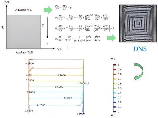
For validation purposes, Figure 3 shows the predicted temperature contours obtained through direct numerical simulation (DNS) using the Rayleigh numbers (Ra) reported by Trias et al. [33]. It is important to note that these authors also used DNS and the finite volume method (FVM) to model natural convection in a cavity with an aspect ratio of A = 4, achieving excellent agreement between the two studies. The temperature contours reveal significant agreement with those documented in the reference work. In both scenarios, the characteristic thermal structures of natural convection in closed cavities are evident, demonstrating complex convective circulation driven by the thermal gradient between the hot and cold walls. For Ra = 6.4 × 10⁸, a relatively stable convective pattern is observed, characterized by well-defined thermal layers and smooth transitions between high- and low-temperature regions, indicating that turbulence has not yet entirely dominated the fluid flow.

As Ra increases to 2 × 10⁹, the thermal layers start to deform due to stronger convective effects, leading to more irregularities in the isotherms, which indicates the beginning of the transition to turbulence. The comparison with the results reported by Trias et al. [33] shows a similar trend, confirming that direct numerical simulation (DNS) can effectively capture these phenomena. At Ra = 10¹⁰, the flow becomes fully turbulent, as shown by the more irregular isotherms and increased thermal mixing within the cavity, along with the development of extremely fine thermal boundary layers along the hot and cold walls—a typical feature of high-Ra flows. Compared to the results of Trias et al. [33], the overall structure of the temperature contours remains consistent, although slight differences may exist due to mesh refinement and the discretization methods used in both studies. In conclusion, the comparison of the temperature contours obtained in this study with those reported by Trias et al. [33] confirms the validity of the direct numerical simulation used here, clearly illustrating the evolution of the thermal flow structure as Ra increases—from more stable configurations at Ra = 6.4 × 10⁸ to fully turbulent flow at Ra = 1 × 10¹⁰. This indicates that the mesh and numerical methods employed are suitable for modeling natural convection effects at high Rayleigh numbers, increasing confidence in the accuracy of the results [34].

In addition to the qualitative comparison of thermal contours, a quantitative evaluation of the results was conducted using the average Nusselt number calculated along the hot wall.

Table 3. Comparison of the average Nusselt numbers calculated in this work with those reported by Trias et al. [33] for different Rayleigh numbers.

Ra	$\overline{\mathbf{N}\mathbf{u}}$ This Work	$\overline{\mathbf{N}\mathbf{u}}$ Reported by Trias et al. [33]
6.4 × 108	49.98	49.23
2 × 109	65.78	66.19
1 × 1010	98.20	100.60

presents the values obtained in this study and those reported by Trias et al. [33] for similar Rayleigh numbers. For Ra = 6.4 × 10⁸, the Nusselt number calculated in this work was 49.98, while Trias et al. [33] reported a value of 49.23, resulting in a relative difference of only 1.52%. For Ra = 2 × 10⁹, the value obtained was 65.78, compared to 66.19 reported by Trias et al. [33], representing a difference of 0.62%. Finally, for Ra = 1 × 10¹⁰, the Nusselt number was 98.2, whereas Trias et al. [33] reported 100.6, yielding a difference of 2.39%. These minor discrepancies are within the expected range. These differences can be attributed to variations in mesh refinement, numerical schemes, and convergence criteria, all of which can have a slight influence on the prediction of thermal flow in the turbulent regime. Nonetheless, the excellent agreement between both studies—both in the temperature contours and in the calculated Nusselt numbers—confirms the validity and accuracy of the direct numerical simulation (DNS) employed in this work, as well as the model’s ability to reliably reproduce the thermal behavior of natural convection at high Rayleigh numbers.

Building on the modeling approach previously described, this study was conducted under steady-state assumptions, utilizing spatially averaged values obtained from fully converged numerical results. In contrast, Trias et al. [33] performed unsteady simulations, averaging results over time once a statistically steady regime was reached. In these cases, flow quantities oscillate around stable mean values, and the Nusselt number is derived from temporal integration. Despite the differences in averaging methods, the close match in both thermal distributions and average Nusselt numbers confirms the accuracy of this numerical strategy and its effectiveness in capturing natural convection behavior at high Rayleigh numbers.

3.2. Nusselt Number

From an applied perspective, one of the most relevant parameters for quantifying heat transfer efficiency in convection systems is the Nusselt number (Nu). This dimensionless number measures the additional heat transferred due to fluid motion (natural convection) compared to the heat transferred by conduction alone if the fluid were at rest. In the context of differentially heated cavities, where the fluid remains confined and the lateral walls are maintained at different temperatures, the Nusselt number provides a direct measure of the intensity of convective circulation induced by temperature gradients and is determined as follows.

$$\overline{\mathrm{N}\mathrm{u}}={\int }_0^1{\left.-{\displaystyle \frac{\partial \theta }{\partial X}}\right|}_{X=0}dY$$

(39)

To evaluate the accuracy of the temperature profiles calculated using direct numerical simulation (DNS) and those obtained with the κ-ε turbulence model, the percentage difference between the average Nusselt numbers was computed as a function of the Rayleigh number. As shown in

Table 4. Comparison of the average Nusselt number calculated using DNS vs. that obtained with the κ-ε turbulence model.

Ra	103	104	105	106	107	108	109	1010
DNS	1.12	2.24	4.52	8.83	16.53	30.23	54.89	100.01
κ-ε	1.06	2.30	5.32	10.54	19.46	34.16	57.97	98.85
Error %	5.17	2.45	17.64	19.39	17.70	12.98	5.61	1.16

, for Ra = 10³ and Ra = 10⁴, within the laminar regime, the percentage differences are moderate, with values of 5.17% and 2.45%, respectively. However, these differences increase significantly to 17.64% for Ra = 10⁵ and 19.39% for Ra = 10⁶. This trend is attributed to the inability of the κ-ε model to adequately characterize the dominant diffusive effects in the thermal boundary layers, whose resolution is critical in flows with strong conduction–convection interaction, as occurs within this Rayleigh number range [3,4,8,9,18]. This limitation arises from the isotropic nature of the turbulent viscosity formulation in the κ-ε model, which fails to capture the intense thermal gradients and the anisotropic structures that develop within the boundary layer, particularly near the hot and cold walls, where heat transport is highly localized. In contrast, DNS directly resolves the flow dynamics without needing closure models, allowing for a more accurate representation of boundary layer thinning and its impact on the Nusselt number. As the Rayleigh number increases beyond Ra = 10⁶, the flow becomes fully turbulent, and the κ-ε model behaves more consistently. For Ra = 10⁷ and Ra = 10⁸, the percentage difference decreases to 17.70% and 12.98%, respectively, indicating a gradual improvement in the prediction of heat transfer. This improvement can be attributed to the fact that, within this range, turbulent effects begin to dominate over conductive mechanisms, making the κ-ε model more representative of the actual flow physics.

Finally, for Ra = 10⁹ and Ra = 10¹⁰, excellent agreement is observed between both approaches, with reduced errors of 5.61% and 1.16%, respectively. These results indicate that the κ-ε model can adequately capture the global flow behavior under fully developed turbulent conditions, where convective transport predominates and the thermal boundary layers, although thin, exhibit dynamics better represented by the turbulence model formulation.

Table 5. Comparison of the average Nusselt number calculated using DNS in laminar flow versus those reported by other authors.

Rayleigh Number
Authors	103	104	105	106	107	108	109	1010
De Vahl Davis, [1] Finite Difference Method	1.50	3.52	4.51	8.79	------	------	------	------
Markatos and Pericleous, [5] Finite volume approach	3.54	3.48	4.43	8.7	------	32.0	------	156.8
Barakos et al. [3] Finite-Domain Equations	1.11	2.24	4.51	8.81	------	30.1	54.4	97.6
Dixit and Babu, [13] Lattice Boltzmann method	1.12	2.28	4.54	8.65	16.79	30.5	57.3	103.6
Goloviznin et al. [8] CABARET scheme	1.17	2.23	4.51	8.82	------	30.3	55.6	100.3
Hernández-López et al. [9] Lattice Boltzmann method	1.11	2.24	4.45	8.86	-----	-----	58.0	137.7
Molina-Herrera et al. [2] Orthogonal collocation method	1.11	2.24	4.51	8.82	16.51	30.2	------	-------
This Work Finite Element Method	1.12	2.24	4.52	8.83	16.53	30.23	54.89	100.01
Validation of the average Nusselt number using Orthogonal Collocation Method.	1.11	2.24	4.51	8.80	16.48	30.13	54.31	-------

compares the average Nusselt numbers reported by various authors with those calculated in this study as a function of the Rayleigh number, which ranges from Ra = 10³ to Ra = 10¹⁰. In addition to these results, Table 5 includes the numerical methods used by each author, enabling an analysis of the differences between these approaches. The table shows that the values obtained in this study demonstrate excellent agreement with reference results from the literature, particularly those reported by Dixit and Babu [13] and Goloviznin et al. [8], who utilized high-accuracy schemes to solve natural convection in two-dimensional square cavities. The range 10³ ≤ Ra ≤ 10⁸, the Nusselt numbers calculated in this work closely aligned with previous studies, validating the precise resolution of thermal boundary layers and the appropriate treatment of boundary conditions in the current model.

Additionally, for validation purposes, the natural convection problem described in this study was also solved using the orthogonal collocation method with Legendre polynomials, employing the computational code NEWCOL2L (written in FORTRAN 90) with a 71 × 71 node mesh, achieving Rayleigh numbers up to 10⁹ through DNS. The discretized equations were solved using the modified Newton method [35] with LU factorization, and the partial derivatives of the Jacobian matrix were approximated using finite differences. A detailed description of the procedure can be found in Molina-Herrera et al. [2]. Table 3 compares the average Nusselt numbers obtained using the orthogonal collocation method with those calculated in this study, demonstrating excellent agreement. This validates the mesh employed, as the results demonstrate remarkable consistency regardless of the numerical method used.

It is important to note that experimental data for validation were not available in this numerical study. Table 5 presents a comparative analysis of the average Nusselt numbers obtained through DNS in the current work alongside those reported in the literature by various authors using different numerical methods. This comparison includes values collected via finite volume, finite element, and spectral methods across a wide range of Rayleigh numbers. Additionally, the present DNS results were verified using the orthogonal collocation method implemented in Fortran through the NEWCOL2L code [35], utilizing Legendre Polynomials with a 71 × 71 mesh. Although these results are not experimental, they provide a reliable verification framework that supports the accuracy and consistency of the numerical solutions presented in this study, particularly at high Rayleigh numbers where boundary layer resolution is critical.

3.3. Macroscopic Energy Balance

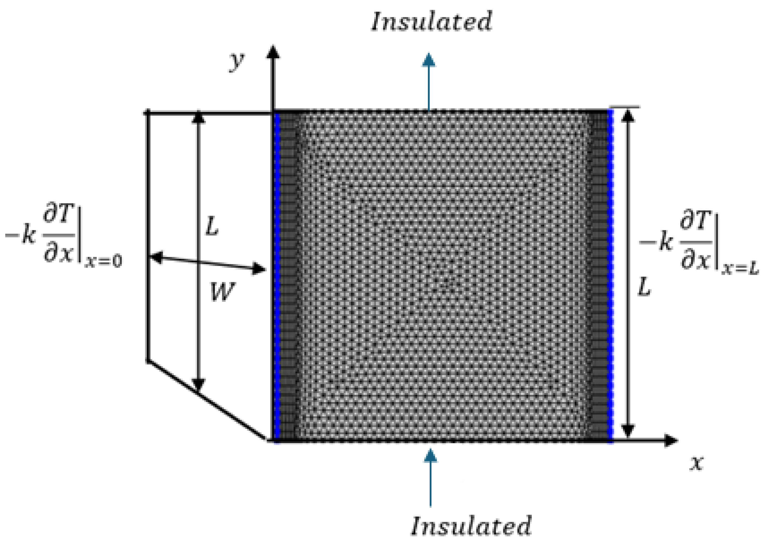
Another criterion for validating the accuracy of the numerical method involves calculating the percentage error in the macroscopic energy balance for a two-dimensional square cavity with adiabatic top and bottom walls, as illustrated in Figure 4. Under these conditions, the macroscopic energy balance confirms that the heat transferred by convection from the hot wall into the fluid must equal the heat leaving the cavity through the cold wall [2]. This comparison is made by quantifying the net heat flux at the walls using Expressions (40)–(42).

$$Q_{In}={\int }_0^W{\int }_0^L\left({\left.-k{\displaystyle \frac{\partial T}{\partial x}}\right|}_{x=0}\right)dydz+{\int }_0^W{\int }_0^L\left({\left.-k{\displaystyle \frac{\partial T}{\partial y}}\right|}_{y=0}\right)dxdz$$

(40)

$$Q_{Out}={\int }_0^W{\int }_0^L\left({\left.-k{\displaystyle \frac{\partial T}{\partial x}}\right|}_{x=L}\right)dydz+{\int }_0^W{\int }_0^L\left({\left.-k{\displaystyle \frac{\partial T}{\partial y}}\right|}_{y=L}\right)dxdz$$

(41)

$$\% error=\left|{\displaystyle \frac{Q_{In}-Q_{Out}}{Q_{In}}}\right|\times 100$$

(42)

The heat flow in the horizontal walls should be zero. As the solution is numerical, the expected values should be minimal concerning the Nusselt number in question. Therefore, it is also necessary to evaluate them to ensure that the calculated Nusselt number is accurate.

Table 6. Comparison of macroscopic energy balance percentage errors calculated using DNS versus those obtained with the κ-ε turbulence model.

Ra	103	104	105	106	107	108	109	1010
DNS	0.0000	0.0000	0.0000	0.0000	0.0001	0.0004	0.0003	0.0018
κ-ε	0.0000	0.0000	0.0001	0.0002	0.0003	0.0002	0.0004	0.0018
OCM	6.028 × 10−6	1.028 × 10−5	1.20 × 10−5	1.4610−5	1.79 × 10−5	2.20 × 10−5	2.71 × 10−5	-----

presents the macroscopic energy balance calculated using direct numerical simulation (DNS) and the κ-ε turbulence model. In the DNS results, the balance remains effectively zero up to intermediate Rayleigh numbers (Ra ≤ 10⁶), with slight increases of 0.0001, 0.0004, 0.0003, and 0.0018 observed at higher Rayleigh numbers (10⁷ ≤ Ra ≤ 10¹⁰), which confirms the global conservation of energy, and the precision of the mesh employed. In contrast, the κ-ε model maintains a zero balance in laminar regimes, exhibiting moderate increases of 0.0002 and 0.0003 during transitions to higher Rayleigh numbers, with values that match those obtained by DNS in the most demanding cases. This consistency indicates that direct numerical simulation can accurately capture both laminar and turbulent regimes. At the same time, the κ-ε model provides comparable results, thereby validating the numerical strategy and mesh design used in this study. Moreover, the κ-ε model exhibits a zero balance in laminar regimes (Ra ≤ 10⁴), with moderate increases of 0.0002 and 0.0003 as the flow transitions to higher Rayleigh numbers (Ra ≥ 10⁵), reaching values identical to those of DNS at Ra = 10⁹ and 10¹⁰. This agreement further supports the hypothesis that DNS can precisely capture both laminar and turbulent regimes. At the same time, the κ-ε model delivers comparable outcomes, confirming the effectiveness of the numerical approach and meshing strategy employed.

Nevertheless, the global errors in the κ-ε model remain at small values. Its more stable performance under high Rayleigh conditions can be explained by the model’s average nature, which filters out high-frequency fluctuations and prioritizes macroscopic energy conservation, albeit at the cost of reduced local accuracy in the velocity and temperature profiles. This observation aligns with findings reported by Wilcox [11], who noted that RANS models tend to exhibit a good global energy balance [16,32].

As in the validation of the Nusselt number, the NEWCOL2L code was also used to evaluate the percentage errors in the macroscopic energy balance using direct numerical simulation (DNS). Table 5 shows that these errors are minor and tend to approach zero within the range of 10³ ≤ Ra ≤ 10¹⁰, validating global energy conservation within the cavity. This behavior is attributed to the orthogonal collocation method, which discretizes the differential operators from boundary to boundary, resulting in high accuracy [25]. Under these conditions, the energy balance error is practically negligible, although CPU time remains significant. While the percentage errors obtained with DNS and the κ-ε turbulence model stay within an acceptable range, the results underscore the importance of finer mesh refinement in boundary regions, particularly where intense thermal gradients occur. However, due to current computational limitations, achieving this level of refinement may be impractical for simulations at higher Rayleigh numbers.

Table 7. Comparison of macroscopic energy balance percentage errors calculated using DNS for different numbers of boundary layers at the walls.

Ra	BL = 6	BL = 8	BL = 10	Ra	BL = 6	BL = 8	BL = 10
103	0.0000	0.0000	0.0000	107	0.0022	0.0001	0.0001
104	0.0000	0.0000	0.0000	108	0.0034	0.0004	0.0004
105	0.0000	0.0000	0.0000	109	0.0013	0.0003	0.0003
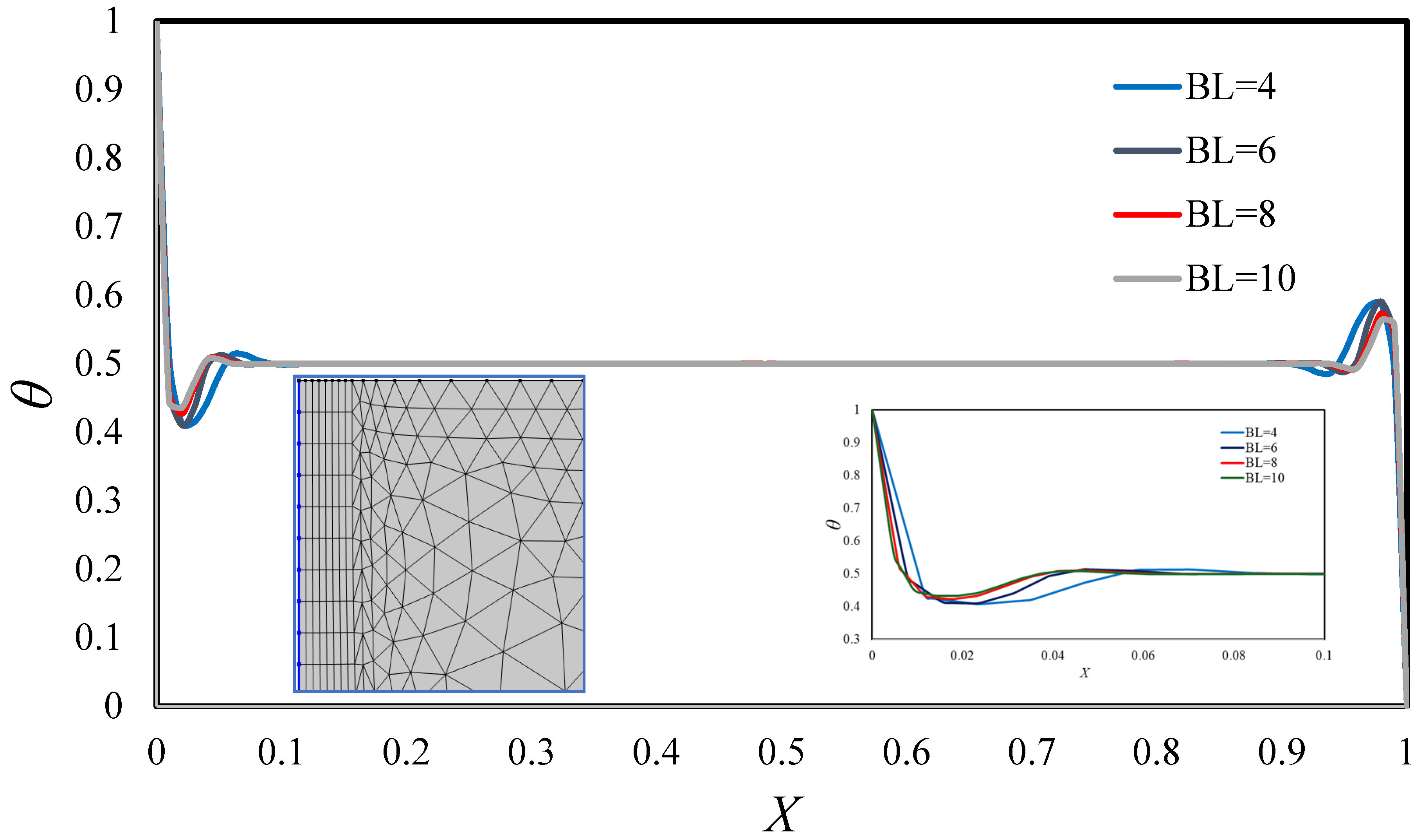
106	0.0002	0.0002	0.0000	1010	0.0023	0.0018	0.0018

compares the percentage errors in the macroscopic energy balance calculated using direct numerical simulation (DNS) across various mesh configurations, with the number of boundary layers ranging from 6 to 10, a stretching factor of 2, a total layer thickness of 0.01 m, and an Extremely Fine mesh. This comparison enables the assessment of the impact of local refinement in critical regions of the domain, particularly along the hot and cold walls, where significant thermal gradients are present. The results indicate that while the reduction in error is notable when increasing from 6 to 8 boundary layers, the difference between 8 and 10 layers becomes minimal. This suggests that beyond 8 layers, the model sufficiently captures boundary layer dynamics without requiring further refinement, which would otherwise increase computational costs. Therefore, the configuration with 8 boundary layers is optimal, providing an efficient balance between numerical accuracy and computational demand. Furthermore, for Ra = 10¹⁰, for BL = 8 and BL = 10, the error in the overall energy balance is practically 0.00183%. However, the CPU time is smaller for BL = 8, which confirms the effectiveness of the mesh optimization.

3.4. Comparison of Temperature and Velocity Profiles Between DNS and the κ-ε Model

Continuing the analysis of the differentially heated square cavity, Figure 5 shows the evolution of the dimensionless temperature profiles along the cavity length (X), comparing results from direct numerical simulation (solid lines) with those from the κ-ε turbulence model (dash-dotted lines). For Ra = 10³, the flow is fully conductive, as indicated by the straight green lines, with a 2.59% difference between the two models. This difference grows to 5.14% for Ra = 10⁴ and 5.8% for Ra = 10⁵. The most significant difference occurs at Ra = 10⁶, reaching 12.5%, indicating that the κ-ε model underestimates the temperature near the walls due to turbulent viscosity, which reduces the conductive contribution in the thermal boundary layer of the energy equation. This behavior aligns with the findings of Barakos et al. [3], who reported that the κ-ε turbulence model accurately reproduces flow characteristics at high Ra but exhibits deviations near the walls in laminar or transitional regimes. Starting with Ra = 10⁷, the difference between the models decreases sharply, and for Ra = 10⁸, only a tiny difference of 0.05% is observed, indicating excellent agreement between DNS and the κ-ε model. This result aligns with the findings of Hernández-López et al. [9], who demonstrated that both approaches produce similar thermal profiles in turbulent regimes dominated by advective convection.

To examine this behavior in detail, Figure 6 presents the dimensionless temperature profiles for high Rayleigh numbers in the range of 10⁹ ≤ Ra ≤ 10¹⁰. In these cases, the profiles obtained via direct numerical simulation (DNS) and those calculated using the κ-ε turbulence model are nearly identical, demonstrating strong agreement between the two methods under fully turbulent conditions. This behavior reinforces the previously observed trend, in which the discrepancy between the two models diminishes as the flow moves away from the transitional regime and advective convection becomes the dominant heat transfer mechanism.

These results are highly consistent with those reported by other authors in the literature [7,8,18,19,33,34], who concluded that under high Rayleigh number conditions and fully developed turbulent flow, turbulence models such as κ-ε can adequately capture the global thermal behavior without the need to resolve all flow scales, as DNS does. Similarly, Trias et al. [33], applying DNS in a cavity with a geometric aspect ratio of 4 for Rayleigh numbers ranging from 6.4 × 10⁸ to 1 × 10¹⁰, observed that the temperature distribution exhibits clear stratification in the center and intense thermal gradients within the boundary layers—both of which are accurately described by DNS and RANS models, given that the mesh is sufficiently refined. Barakos et al. [3] also emphasized that temperature profiles tend to stabilize in strongly convective regimes, and the differences between turbulence models and DNS decrease significantly if mesh refinement near the walls is adequate to resolve the thermal boundary layers. Overall, the excellent agreement observed in this study for Ra ≥ 10⁹ validates the capability of direct numerical simulation to predict thermal distributions in differentially heated cavities and demonstrates that under fully turbulent conditions, both approaches converge to virtually equivalent solutions [9,13,19].

This behavior also indicates that the global energy balance stabilizes once a sufficient resolution is achieved to capture the transport mechanisms in regions with the highest gradients, thereby validating the implemented numerical scheme.

Regarding the temperature contours, Figure 7 shows those obtained from direct numerical simulation (DNS), while Figure 8 displays the results generated using the κ-ε turbulence models. The analysis focuses on thermal behavior at high Rayleigh numbers in the range of 10⁸ ≤ Ra ≤ 10¹⁰, highlighting the evolution of thermal stratification, boundary layers, and the transition to the turbulent regime. Temperature contours for Ra values from 10³ to 10⁸ have been extensively studied in the literature (authors) and reported in a previous study by Molina-Herrera et al. [2]. Within this Rayleigh range, the flow gradually transitions from conduction-dominated behavior to increasingly intense convection as Ra increases. It is well documented that the rise in the Rayleigh number makes thermal stratification and boundary layer thinning more pronounced. Since these earlier results have been validated in multiple studies, the present work focuses on the thermal behavior for Ra = 10⁸ to 10¹⁰, where the flow reaches a fully turbulent regime and heat transfer is predominantly advective.

These figures show that for Ra = 10⁹, the temperature contours obtained with DNS and the κ-ε turbulence model exhibit significant thermal stratification, displaying intensified temperature gradients along the hot and cold walls. However, the κ-ε model slightly underestimates thermal dissipation near the walls, which aligns with the findings of Hernández-López et al. [9], who noted that RANS models tend to reduce diffusive effects in the boundary layer region. Nevertheless, the similarity in the overall shape of the thermal contours indicates that both models effectively capture the impact of advective convection. Additionally, the studies by Trias et al. [33] demonstrate that, from this Rayleigh number onward, the flow develops small instabilities within the thermal boundary layers, which DNS captures more accurately. In contrast, the κ-ε model produces smoother isotherms, suggesting that turbulent transport is slightly overestimated compared to the DNS solution. As the Rayleigh number rises to Ra = 10¹⁰, thermal stratification becomes even more pronounced, with nearly horizontal isotherms in the center of the cavity. Both models agree that convection is the primary heat transfer mechanism, consistent with findings reported by various authors [13].

A notable difference is that DNS captures the intensity of thermal gradients in the boundary layer more accurately. In contrast, the κ-ε model tends to smooth the profile in this region. This observation aligns with previous studies indicating that turbulence models often overestimate turbulent dissipation, resulting in an artificially thickened thermal boundary layer. Nevertheless, both models exhibit well-defined thermal recirculation zones in the upper region of the cavity, suggesting that the global flow structure is consistently represented in both simulations.

Trias et al. [33] also reported that thermal stratification is nearly complete in this range of Ra, a characteristic evident in both simulations. This indicates that the difference between DNS and the κ-ε model in this regime is primarily quantitative, as the overall flow structure and thermal distribution remain comparable. For Ra = 10¹⁰, the flow achieves a fully turbulent regime, with thermal stratification nearly complete at the center of the cavity [13,19]. DNS and the κ-ε model produce virtually identical isotherms in this scenario, confirming that advective convection entirely dominates heat transfer. Furthermore, the thermal gradients at the hot and cold walls are steep, and the thermal boundary layer is exceedingly thin. Fluid recirculation in the upper part of the cavity intensifies, indicating that thermal energy is rapidly transported upward, consistent with previous findings [9,13,19]. The difference between the two models is minimal, with a discrepancy of less than 0.001% in the dimensionless temperature values at the hot wall. This implies that under this fully turbulent regime, the κ-ε model and DNS practically converge to the same solution. In terms of overall comparison, for Rayleigh numbers of 10⁹ and 10¹⁰, the κ-ε model tends to overestimate thermal dissipation in the boundary layer compared to DNS. For Ra = 10¹⁰, the thermal structure is similar in both models, although DNS captures the boundary layer gradients more accurately.

Figure 9 illustrates the velocity profiles of the Uy component along the horizontal X-axis for Rayleigh numbers ranging from 10³ to 10¹⁰, obtained through direct numerical simulation (DNS) and the κ-ε turbulence model. The solid lines represent the results from DNS, while the dashed lines correspond to the predictions from the κ-ε model. For both models, it is noted that the magnitude of Uy increases as the Rayleigh number rises, indicating a strengthening of convective flow within the cavity. For Ra ≤ 10⁵, the velocity profiles obtained from DNS exhibit a parabolic shape near the walls, with peak values in those regions and a minimum at the center of the cavity, suggesting strong recirculation. As the Rayleigh number increases, starting from Ra = 10⁶, the profiles gradually thin the boundary layer and transition towards nearly linear shapes, characteristic of regimes where convection strongly dominates over thermal diffusion. For Ra ≥ 10⁸, the profile becomes almost linear, indicating a highly stratified and advective flow [18].

In contrast, the velocity profiles predicted by the κ-ε model show significant differences. For Ra = 10³, the profile is nearly linear. It fails to reproduce the expected parabolic shape, indicating a poor representation of laminar flow due to the excessive turbulent dissipation characteristic of this model. As Ra increases, the κ-ε model starts to capture parabolic-type profiles near the differentially heated walls, particularly for Ra ≥ 10⁵. However, this behavior does not resemble the pattern observed with DNS; unlike the latter, the κ-ε velocity profiles maintain parabolic shapes even at high Rayleigh numbers, which contradicts the tendency toward linear profiles characteristic of the dominant advective regime. This discrepancy suggests that the κ-ε model struggles to capture the flattening of the central profile adequately and tends to produce pronounced velocity gradients near the heated walls, limiting its accuracy in predicting flow in differentially heated cavities. Overall, these results confirm that while the κ-ε model is helpful in highly turbulent regimes, its ability to represent flow dynamics accurately is limited in laminar and transitional regimes, where DNS provides a more precise description in both magnitude and shape of the velocity profiles [9,13,19,20].

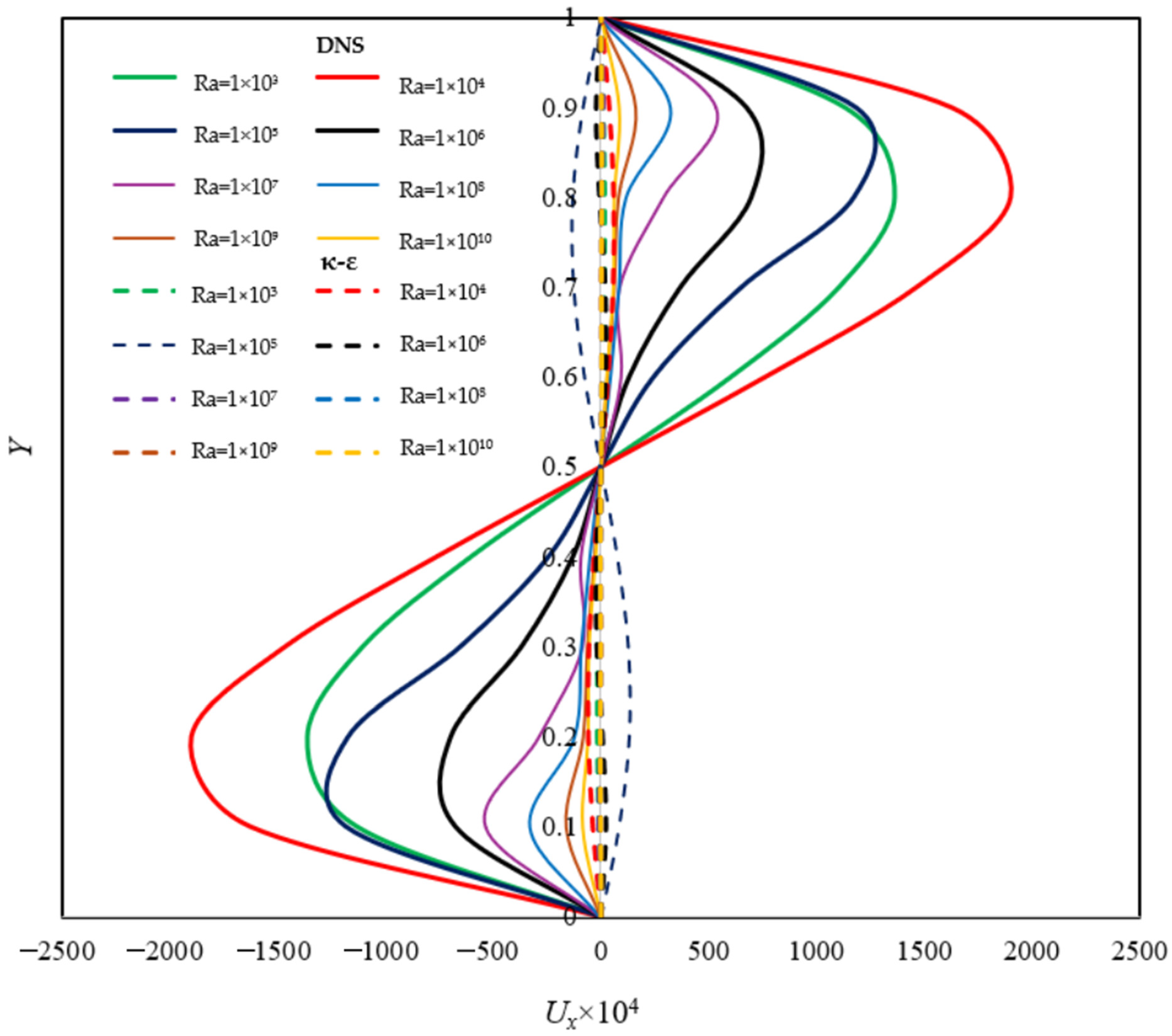
Extending the analysis, Figure 10 shows the velocity profiles of the horizontal component Ux along the cavity height (Y), as predicted by direct numerical simulation (DNS) and the κ-ε turbulence model. As in the previous figure, solid lines represent DNS results, while dashed lines correspond to κ-ε predictions. The DNS-calculated profiles exhibit a symmetric, parabolic shape with well-defined peaks near the upper and lower walls (regions close to Y = 0 and Y = 1). This behavior is typical of laminar flows with established natural convection, generally observed for Ra ≤ 10⁵, where convection begins to dominate over thermal diffusion. In this regime, intense flow is generated along the horizontal walls, with maximum velocities linked to the upward motion of hot fluid near the right wall and the downward motion of cold fluid near the left wall. As the Rayleigh number increases (Ra ≥ 10⁶), a progressive reduction in the Ux velocity magnitude occurs in the central region of the cavity. This trend continues with increasing Ra, and for very high values (Ra ≥ 10⁹), the profiles tend to flatten, and the Ux component approaches zero throughout the cavity height [18]. This phenomenon can be explained by the intensification of the advective nature of the flow: as the Rayleigh number increases, motion within the cavity becomes increasingly concentrated in narrow thermal boundary layers adjacent to the vertical walls, significantly reducing the magnitude of horizontal flow in the cavity core. In this strongly stratified regime, natural convection generates dominant vertical flows, while horizontal components diminish, resulting in near-zero Ux velocities outside the boundary layers [18,22,23,24].

In contrast, the velocity profiles predicted by the κ-ε model show notable discrepancies when compared to those obtained with DNS. For Ra = 10³, the profiles are significantly smoother and do not capture the characteristic parabolic structures observed with DNS. This reduction in Ux velocity component values results from the nature of the κ-ε model, which introduces turbulent kinetic energy dissipation (ε), particularly significant in laminar and transitional regimes. In these regimes, the production of turbulent kinetic energy (κ) is nearly zero due to the lack of strong fluctuations in the flow, causing dissipation to far exceed production and thereby reducing the intensity of the velocity profiles. As the Rayleigh number increases, the Ux velocity values tend to become nearly linear, approaching values close to zero over much of the domain. This behavior is attributed to the predominant dissipation of turbulent kinetic energy (ε) and the low production of energy (κ), which restricts the development of intense turbulent structures in areas distant from the walls, especially in the cavity center. Furthermore, the formation of thin boundary layers near the walls, where convective flow prevails, concentrates velocity gradients in these regions. In contrast, the flow in the interior of the domain becomes more uniform [13,14,19].

Furthermore,

Table 8. Comparison of the maximum velocities calculated in this study with those reported by other authors.

	De Vahl Davis [1]		Goloviznin et al. [8]		This Work
Ra	Ux, max × 103 (Y)	Uy, max × 103 (X)	Ux, max × 103 (Y)	Uy, max × 103 (X)	Ux, max × 103 (Y)	Uy, max × 103 (X)	Nu This Work	Deviations from Goloviznin et al. [8]
103	3.496 (0.813)	3.697 (0.178)	3.596 (0.829)	3.677 (0.171)	3.459 (0.821)	3.650 (0.168)	1.1178	0.626%
104	16.178 (0.823)	19.617 (0.0119)	15.927 (0.829)	19.516 (0.125)	15.662 (0.829)	19.372 (0.123)	2.2449	0.178%
105	34.730 (0.855)	68.590 (0.066)	38.542 (0.872)	67.265 (0.0531)	35.458 (0.883)	67.24 (0.0561)	4.5221	0.088%
106	64.630 (0.850)	219.36 (0.0379)	74.125 (0.893)	219.941 (0.0333)	72.512 (0.890)	217.475 (0.0301)	8.8281	0.022%
107	----------------	-----------------	167 (0.893)	701 (0.0175)	163.571 (0.898)	694.515 (0.0170)	16.534	0.420%
108	----------------	-----------------	482 (0.893)	2100 (0.086)	489.542 (0.921)	2149 (0.0842)	30.236	0.033%
109	---------------	-----------------	1020 (0.9667)	6700 (0.086)	1078 (0.9821)	6878 (0.08012)	54.889	0.852%
1010	----------------	-----------------	2100	22,000	2189 (0.9981)	21,578(0.05311)	100.01	0.947%

presents the maximum velocities of the dimensionless components Ux and Uy, calculated using direct numerical simulation (DNS) and compared with the values reported by De Vahl Davis [1] for Rayleigh numbers Ra ≤ 10⁶, as well as the results obtained by Goloviznin et al. [8] for Ra ≥ 10⁷. The maximum velocity values for each component were determined along lines perpendicular to the respective directions (i.e., Ux along a vertical line at X = 0.5 and Uy along a horizontal line at Y = 0.5), locating the local maxima within the domain, with their coordinates given in parentheses. Additionally, the table presents the average Nusselt numbers and their percentage deviations from the benchmark values of De Vahl Davis [1] and Goloviznin et al. [8]. Table 8 shows that direct numerical simulation, when implemented with mesh refinement along the differentially heated walls, provides results consistent with those of De Vahl Davis up to Ra = 10⁶, with deviations below 1% in the Nusselt number, thereby validating the accuracy of the numerical model in the laminar regime. However, for higher Rayleigh numbers (Ra ≥ 10⁹), the maximum velocity values tend to shift toward the region near the upper wall and closer to the hot wall T_h. This difference is attributed to the mesh refinement in the near-wall regions, which enables better resolution of thermal and velocity boundary layers, causing the zones of highest convective transport and maximum velocity to concentrate in narrower regions closer to the hot boundaries. Overall, the results confirm that the numerical strategy employed is suitable for both the laminar regime and the transition to turbulent flow, accurately capturing the maximum velocities and the characteristic flow structures of natural convection in differentially heated cavities.

Meanwhile,

Table 9. Comparison of the maximum velocities calculated with DNS versus those predicted by the κ-ε model.

	DNS		κ-ε
Ra	Ux, max × 103 (Y)	Uy, max × 103 (X)	Ux, max × 103 (Y)	Uy, max × 103 (X)	Ux, Error	Uy, Error
103	3.459 (0.821)	3.650 (0.168)	2.712 (0.863)	3.850 (0.116)	21.59%	0.0547%
104	15.662 (0.829)	19.372 (0.123)	14.751 (0.843)	22.372 (0.102)	5.816%	0.1548%
105	35.458 (0.883)	67.24 (0.0561)	30.524 (0.912)	62.24 (0.0431)	13.915%	0.0743%
106	72.512 (0.890)	217.475 (0.0301)	68.381 (0.924)	210.475 (0.0214)	5.696%	0.0321%
107	163.571 (0.898)	694.515 (0.0170)	158.525 (0.945)	684.515 (0.0122)	3.084%	0.0143%
108	489.542 (0.921)	2149 (0.0842)	459.597 (0.991)	2049 (0.0612)	6.116%	0.0465%
109	1078 (0.9821)	6878 (0.08012)	1025.003(0.993)	6478 (0.07898)	4.916%	0.0581%
1010	2189 (0.9981)	21,578 (0.05311)	2014.25 (0.998)	20,032(0.05174)	7.983%	0.0716%

compares the dimensionless maximum velocities of the Ux and Uy components, obtained using direct numerical simulation (DNS) and the standard κ-ε turbulence model, for different Rayleigh numbers. The maximum values were computed in the same way as in the previous analysis, specifically along lines perpendicular to each velocity component. The results indicate that, for low Rayleigh numbers (Ra ≤ 10⁵), the maximum velocities predicted by the κ-ε model exhibit significant discrepancies when compared to those obtained using DNS. This deviation can be attributed to the excessive dissipation of turbulent kinetic energy in regimes where turbulence effects are not yet fully developed, which limits the model’s ability to predict the flow pattern accurately. As Ra increases (Ra ≥ 10⁷), the differences between both methodologies progressively decrease, suggesting that the κ-ε model becomes more accurate in capturing the main flow features once the turbulent regime is fully established. This behavior confirms that the κ-ε model tends to underestimate maximum velocities in laminar and transitional regimes, due to its formulation based on assumptions of fully developed turbulence. However, in fully turbulent regimes, its predictions closely match those of DNS in both magnitude and spatial location.

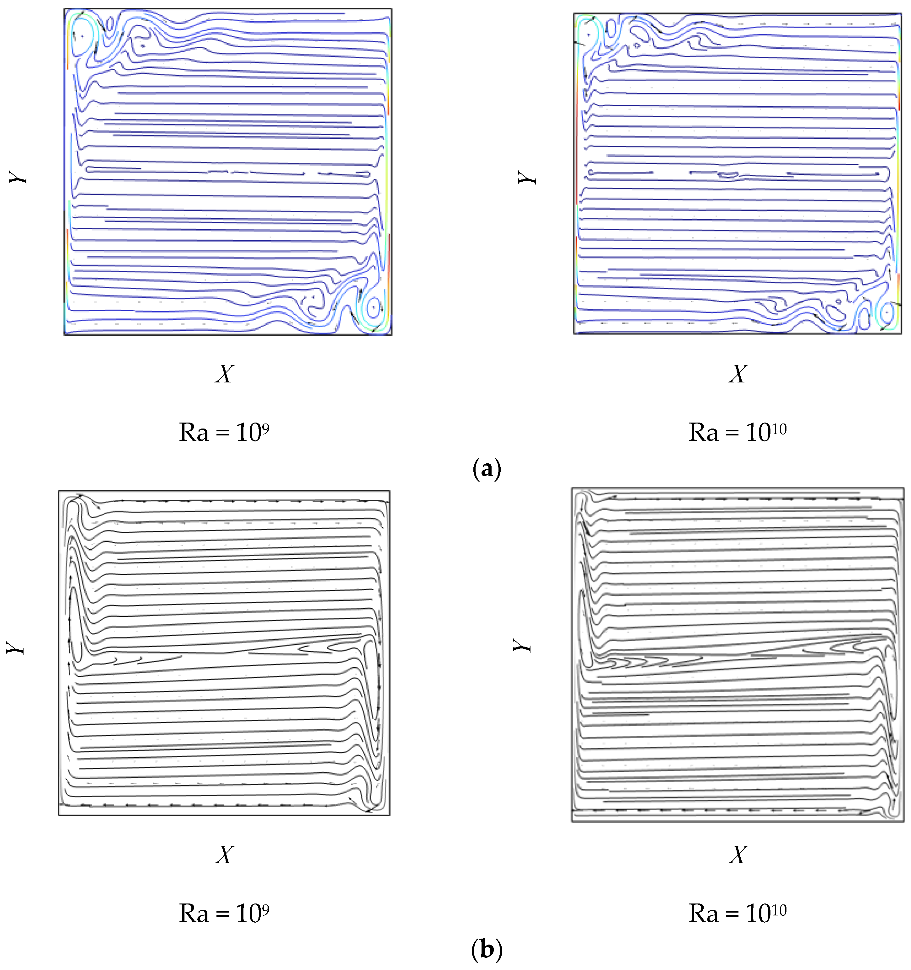
Finally, Figure 11 presents the streamlines obtained for Rayleigh numbers of Ra = 10⁹ and Ra = 10¹⁰, calculated using direct numerical simulation (DNS) and the κ-ε turbulence model. For Ra = 10⁹, the streamlines obtained with DNS reveal a fully turbulent flow characterized by the formation of well-defined vortices in the upper left and lower right corners of the cavity. These recirculation zones indicate intense convective activity associated with the interaction between thin thermal boundary layers and strong velocity gradients. The remainder of the cavity displays parallel and flat streamlines, reflecting a highly convective and stratified regime. For Ra = 10¹⁰, a similar but more intense pattern is observed: the corner vortices become more compact, and the streamlines in the core of the cavity remain horizontal and densely clustered. This behavior is typical of flows at high Rayleigh numbers, where viscous dissipation is localized within thin boundary layers, while the fluid core moves almost inertially.

In contrast, the streamlines generated by the κ-ε model for the identical Rayleigh numbers do not demonstrate clear vortex formation in the cavity corners. Instead, a smoother and more symmetric configuration is observed, with streamlines extending almost continuously in the horizontal direction. This absence of localized vorticity can be attributed to the inadequate representation of small-scale velocity fluctuations, as the κ-ε model tends to overestimate turbulent kinetic energy dissipation (ε) and underestimate its production (κ). Consequently, the model excessively smooths the flow structures, hindering its ability to capture the recirculation mechanisms under high natural convection conditions accurately. This limitation impacts the model’s accuracy in predicting flow patterns in cavities where thin thermal boundary layers and dynamic stratification are significant factors.

It is also important to mention that in previous studies reported by Molina-Herrera et al. [2], streamlines were analyzed for Rayleigh numbers ranging from 10³ to 10⁸, using both direct numerical simulation (DNS) and turbulence models. In these regimes, particularly for Ra ≤ 10⁵, the streamlines obtained through DNS displayed a single dominant recirculation cell centered in the cavity, with smooth and symmetric trajectories indicating a well-organized laminar flow, primarily driven by conduction with the onset of natural convection. As the Rayleigh number increases to the range of 10⁶–10⁸, more complex structures begin to form in the corners, particularly in the lower right and upper left zones, reflecting the emergence of convective instabilities and the transition to more convective flows.

In this context, although it is acknowledged that buoyancy-driven flows at high Rayleigh numbers often develop complex three-dimensional structures, numerous studies have shown that two-dimensional (2D) simulations remain effective for accurately predicting overall quantities such as the Nusselt number and main circulation patterns. Wang et al. [19] and Trias et al. [33] have demonstrated that, with refined meshes and suitable numerical methods, 2D models can reliably reproduce global thermal behavior up to Ra ≈ 10⁹. These simulations are especially valuable for comparing different numerical approaches (such as DNS and κ-ε) in studies where overall accuracy is prioritized over detailed representation of fine three-dimensional structures [27,28]. Specifically, the results presented here indicate that 2D DNS can effectively capture the formation and evolution of corner vortices, which the κ-ε model does not reproduce. This type of 2D analysis provides a solid foundation for assessing the relative performance of various turbulence models and for understanding global transport mechanisms, provided the conclusions remain within the limited scope of this dimensionality.

4. Conclusions

This study shows the effectiveness of the direct numerical simulation (DNS) in resolving natural convection in a differentially heated two-dimensional square cavity across a wide range of Rayleigh numbers (10³ ≤ Ra ≤ 10¹⁰). It employs the finite element method and mesh refinement strategies specifically designed to resolve thermal and hydrodynamic boundary layers. DNS achieves high numerical accuracy, with global macroscopic energy balance errors remaining below 0.0018% throughout the tested range. The κ-ε turbulence model has notable limitations in the laminar and transitional regimes (Ra ≤ 10⁶), overestimating Nusselt numbers by up to 19.39% and maximum velocity magnitudes by up to 13.92%. This is due to its isotropic turbulent viscosity formulation, which fails to capture the anisotropic behavior of near-wall structures and steep temperature gradients.

For Rayleigh numbers Ra ≥ 10⁹, both approaches converged to similar global results, with Nusselt number differences of less than 1.2% and nearly identical temperature profiles and flow patterns. Under fully turbulent conditions, the κ-ε model is computationally efficient and suitable for estimating macroscopic thermal performance. Still, DNS remains essential for resolving fine-scale features and verifying the validity of turbulence models. This work validates DNS as a reference methodology for benchmarking turbulence models in natural convection problems, particularly in geometries where the high spatial resolution of boundary layers is critical. The adopted mesh configuration—with eight boundary layers, a stretching factor of 2.0, and an extremely fine mesh—proved optimal in striking a balance between accuracy and computational cost.

However, the study has several limitations that should be addressed in future work. First, the simulations were performed under steady-state assumptions; extending the analysis to unsteady flows would enable the study of temporal instabilities and chaotic transitions. Second, the current work is limited to two-dimensional domains. While 2D simulations are useful for benchmarking and provide significant insights, fully three-dimensional simulations are necessary to capture secondary instabilities, corner vortices, and 3D effects that become dominant at Ra > 10⁹. Additionally, no experimental validation was possible due to the lack of accessible data under identical conditions. Future challenges include extending DNS to 3D geometries, incorporating transient simulations, and analyzing the influence of different Prandtl numbers and aspect ratios on the onset of turbulence. Furthermore, integrating DNS data with data-driven models (e.g., reduced-order models or machine learning surrogates) can facilitate the development of fast yet accurate prediction tools for engineering design in thermal systems.

References

1. De Vahl Davis, G. Natural convection of air in a square cavity: A benchmark numerical solution. Int. J. Numer. Methods Fluids 1983, 3, 249–264. [Google Scholar] [CrossRef]
2. Molina-Herrera, F.I.; Quemada-Villagómez, L.I.; Navarrete-Bolaños, J.L.; Jiménez-Islas, H. Comparative analysis of nondimensionalization approaches for solving the 2-D differentially heated cavity problem. Int. J. Numer. Methods Fluids 2024, 96, 1276–1303. [Google Scholar] [CrossRef]
3. Barakos, G.; Mitsoulis, E.; Assimacopoulos, D. Natural convection flow in a square cavity revisited: Laminar and turbulent models with wall functions. Int. J. Numer. Methods Fluids 1994, 18, 695–719. [Google Scholar] [CrossRef]
4. Henkes, R.; Hoogendoorn, C. Laminar natural convection boundary-layer flows along a heated vertical plate in a stratified environment. Int. J. Heat Mass Transf. 1989, 32, 147–155. [Google Scholar] [CrossRef]
5. Markatos, N.; Pericleous, K. Laminar and turbulent natural convection in an enclosed cavity. Int. J. Heat Mass Transf. 1984, 27, 755–772. [Google Scholar] [CrossRef]
6. De Vahl Davis, G. Laminar natural convection in an enclosed rectangular cavity. Int. J. Heat Mass Transf. 1968, 11, 1675–1693. [Google Scholar] [CrossRef]
7. Huang, Y.; Yang, G.; Wu, J. Large eddy simulation and experimental study of turbulent mixed convection inside a cavity with large Rayleigh number: Effect of buoyancy. Build Environ. 2019, 151, 268–279. [Google Scholar] [CrossRef]
8. Goloviznin, V.M.; Korotkin, I.A.; Finogenov, S.A. Parameter-free numerical method for modeling thermal convection in square cavities in a wide range of Rayleigh numbers. J. Appl. Mech. Tech. Phys. 2016, 57, 1159–1171. [Google Scholar] [CrossRef]
9. Hernández-López, I.; Xamán, J.; Álvarez, G.; Chávez, Y.; Arce, J. Analysis of laminar and turbulent natural, mixed and forced convection in cavities by heatlines. Arch. Mech. 2016, 68, 27–53. [Google Scholar] [CrossRef]
10. Pérez-Segarra, C.; Oliva, A.; Costa, M.; Escanes, F. Numerical experiments in turbulent natural and mixed convection in internal flows. Int. J. Numer. Methods. Heat Fluid Flow 1995, 5, 13–33. [Google Scholar] [CrossRef]
11. Wilcox, D.C. Turbulence Modeling for CFD; D C W Industries: Mumbai, India, 1993; pp. 201–225. [Google Scholar]
12. Igci, A.A.; Arici, M.E. A comparative study of four low-Reynolds-number k-ε turbulence models for periodically fully developed duct flow and heat transfer. Numer. Heat Transf. B Fundam. 2016, 69, 234–248. [Google Scholar] [CrossRef]
13. Dixit, H.; Babu, V. Simulation of high Rayleigh number natural convection in a square cavity using the lattice Boltzmann method. Int. J. Heat Mass Transf. 2006, 49, 727–739. [Google Scholar] [CrossRef]
14. Weppe, A.; Moreau, F.; Saury, D. Experimental investigation of a turbulent natural convection flow in a cubic cavity with an inner obstacle partially heated. Int. J. Heat Mass Transf. 2022, 194, 123052. [Google Scholar] [CrossRef]
15. Xin, S.; Le Quéré, P. Numerical simulations of 2D turbulent natural convection in differentially heated cavities of aspect ratios 1 and 4. In Fluid Mechanics and Its Applications; Springer: Berlin/Heidelberg, Germany, 1994; pp. 423–434. [Google Scholar] [CrossRef]
16. Fusegi, T.; Hyun, J.M.; Kuwahara, K. Three-dimensional simulations of natural convection in a sidewall-heated cube. Int. J. Numer. Methods Fluids 1991, 13, 857–867. [Google Scholar] [CrossRef]
17. Henkes, R.; Van Der Vlugt, F.; Hoogendoorn, C. Natural-convection flow in a square cavity calculated with low-Reynolds-number turbulence models. Int. J. Heat Mass Transf. 1991, 34, 377–388. [Google Scholar] [CrossRef]
18. Choi, S.; Kim, S. Turbulence modeling of natural convection in enclosures: A review. J. Mech. Sci. Technol. 2012, 26, 283–297. [Google Scholar] [CrossRef]
19. Wang, P.; Zhang, Y.; Guo, Z. Numerical study of three-dimensional natural convection in a cubical cavity at high Rayleigh numbers. Int. J. Heat Mass Transf. 2017, 113, 217–228. [Google Scholar] [CrossRef]
20. Hamadi, B.; Cherrad, M.L.; Boucherma, D.; Chorfi, S.; Boulkroune, S.; Achour, T.; Chaour, M. Numerical study of laminar mixed convection under steady and unsteady flow conditions. South. Fla. J. Dev. 2024, 5, e4663. [Google Scholar] [CrossRef]
21. Ji, Y. CFD Modelling of Natural Convection in air cavities. CFD Lett. 2014, 6, 15–31. Available online: https://usir.salford.ac.uk/id/eprint/35008/ (accessed on 15 March 2024).
22. Cintolesi, C.; Petronio, A.; Armenio, V. Large eddy simulation of turbulent buoyant flow in a confined cavity with conjugate heat transfer. Phys. Fluids 2015, 27, 095104. [Google Scholar] [CrossRef]
23. Germano, M.; Piomelli, U.; Moin, P.; Cabot, W.H. A dynamic subgrid-scale eddy viscosity model. Phys. Fluids A 1991, 3, 1760–1765. [Google Scholar] [CrossRef]
24. Duchaine, F.; Mendez, S.; Nicoud, F.; Corpron, A.; Moureau, V.; Poinsot, T. Conjugate heat transfer with Large Eddy Simulation for gas turbine components. C. R. Mécanique 2009, 337, 550–561. [Google Scholar] [CrossRef]
25. Dorfman, A.; Renner, Z. In Conjugate problems in convective heat transfer: Review. Math. Probl. Eng. 2009, 927350. [Google Scholar] [CrossRef]
26. Bosshard, C.; Dehbi, A.; Deville, M.; Leriche, E.; Puragliesi, R.; Soldati, A. Large eddy simulation of the differentially heated cubic cavity flow by the spectral element method. Comput. Fluids 2013, 86, 210–227. [Google Scholar] [CrossRef]
27. Ghoben, Z.K.; Hussein, A.K. Natural convection inside a 3D regular shape enclosures—A brief review. Int. J. Heat Technol. 2022, 40, 232–246. [Google Scholar] [CrossRef]
28. Hinojosa, J.; Álvarez, G.; Estrada, C. Three-dimensional numerical simulation of the natural convection in an open tilted cubic cavity. Rev. Mex. Fís. 2006, 52, 111–119. Available online: https://www.redalyc.org/pdf/570/57065003.pdf (accessed on 7 March 2024).
29. Hussein, A.K.; Hussain, S.H. Heatline visualization of natural convection heat transfer in inclined wavy cavities filled with nanofluids and subjected to a discrete isoflux heating from its left sidewall. Alex. Eng. J. 2016, 55, 169–186. [Google Scholar] [CrossRef]
30. Selimefendigil, F. Natural convection in a trapezoidal cavity with an inner conductive object of different shapes and filled with nanofluids of different nanoparticle shapes. Iran. J. Sci. Technol. Trans. Mech. Eng. 2018, 42, 169–184. [Google Scholar] [CrossRef]
31. Bird, R.B.; Stewart, W.E.; Lightfoot, E.N. Transport Phenomena, 2nd ed; John Wiley, and Sons, Inc: Hoboken, New Jersey, USA, 2009; p. 928. [Google Scholar]
32. Jones, W.; Launder, B. The prediction of laminarization with a two-equation model of turbulence. Int. J. Heat Mass Transf. 1972, 15, 301–314. [Google Scholar] [CrossRef]
33. Trias, F.X.; Soria, M.; Oliva, A.; Pérez-Segarra, C.D. Direct numerical simulations of two- and three-dimensional turbulent natural convection flows in a differentially heated cavity of aspect ratio 4. J. Fluid Mech. 2007, 586, 259–293. [Google Scholar] [CrossRef]
34. Le Quéré, P. Accurate solutions to the square thermally driven cavity at high Rayleigh number. Comput. Fluids 1991, 20, 29–41. [Google Scholar] [CrossRef]
35. Jiménez-Islas, H.; Calderón-Ramírez, M.; Molina-Herrera, F.; Martínez-González, G.; Navarrete-Bolaños, J.; Castrejón-González, E. Low-RAM algorithm for solving 3-D natural convection problems using orthogonal collocation. Rev. Mex. Ing. Quim. 2014, 13, 259–277. Available online: https://www.redalyc.org/pdf/620/62031166020.pdf (accessed on 4 February 2024).
Figure 1. Geometric system and computational domain.
Modelling 06 00066 g001
Figure 2. Effect of boundary layers on the prediction of dimensionless temperature profiles at the cavity center (θ = 0.5) for Ra = 1010 and A = 1.
Modelling 06 00066 g002
Figure 3. Temperature contours predicted in this work using FEM using the Rayleigh numbers reported by Trias et al. [33].
Modelling 06 00066 g003
Figure 4. Geometric configuration for the macroscopic energy balance.
Modelling 06 00066 g004
Figure 5. Comparison of dimensionless temperature profiles calculated using DNS versus those obtained with κ-ε at the center of the cavity for different Rayleigh numbers in the laminar flow regime.
Modelling 06 00066 g005
Figure 6. Comparison of dimensionless temperature profiles calculated using DNS versus those obtained with κ-ε at the center of the cavity for different Rayleigh numbers in the turbulent flow regime.
Modelling 06 00066 g006
Figure 7. Temperature contours for different Rayleigh numbers calculated using DNS.
Modelling 06 00066 g007
Figure 8. Temperature contours for different Rayleigh numbers calculated using the κ-ε model.
Modelling 06 00066 g008
Figure 9. Comparison of the dimensionless Uy velocity component profiles calculated using DNS versus those obtained with the κ-ε model at the center of the cavity for different Rayleigh numbers.
Modelling 06 00066 g009
Figure 10. Comparison of the dimensionless Ux velocity component profiles computed using DNS and the κ-ε model at the center of the cavity for different Rayleigh numbers.
Modelling 06 00066 g010
Figure 11. Streamlines obtained using (a) DNS (blue isolines) and (b) κ-ε (black isolines).
Modelling 06 00066 g011