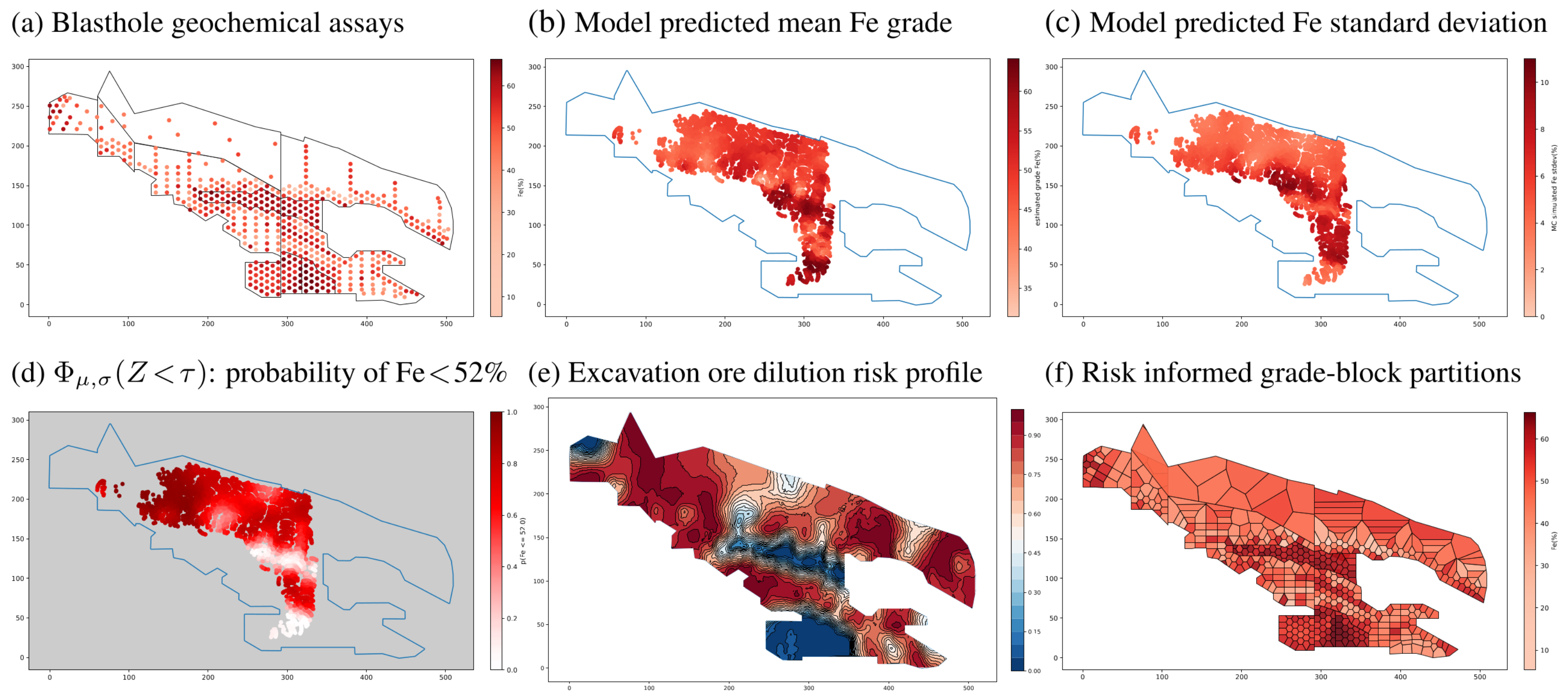
Figure 1.
A motivating example. For open-pit mining at iron ore deposits, (
a) sparse assay measurements are taken from blastholes to facilitate ore grade probabilistic modelling. (
b,
c) These show the estimated mean Fe concentration and standard deviation in a local region soon to be excavated. The value of having a probabilistic model is that it provides a reliable and objective description of ore/waste distribution in spite of sampling errors and epistemic uncertainty. This allows operators to assess risks, such as ore dilution in (
d), if a volume of low-grade material is dug up at a [red] location and transported to a high-grade destination. (
e) A high-fidelity probabilistic model makes informed decision-making possible. Its applications include high-precision large-scale tracking of material movement, as well as (
f) grade-block partitioning and reconfiguration during mine planning and the ability to reroute material to different destinations on demand [
19].
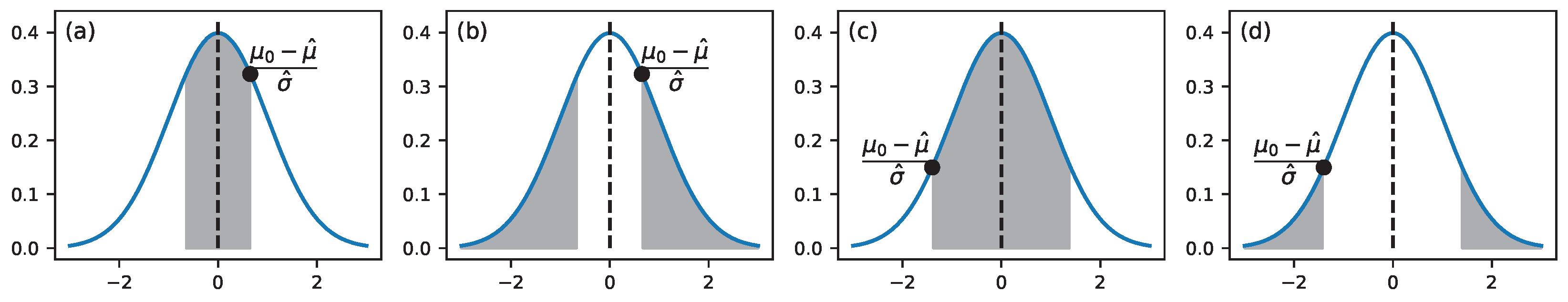
Figure 2.
Illustration of coverage probability in (a,c) and consensus between model and observation in (b,d).
Figure 2.
Illustration of coverage probability in (a,c) and consensus between model and observation in (b,d).
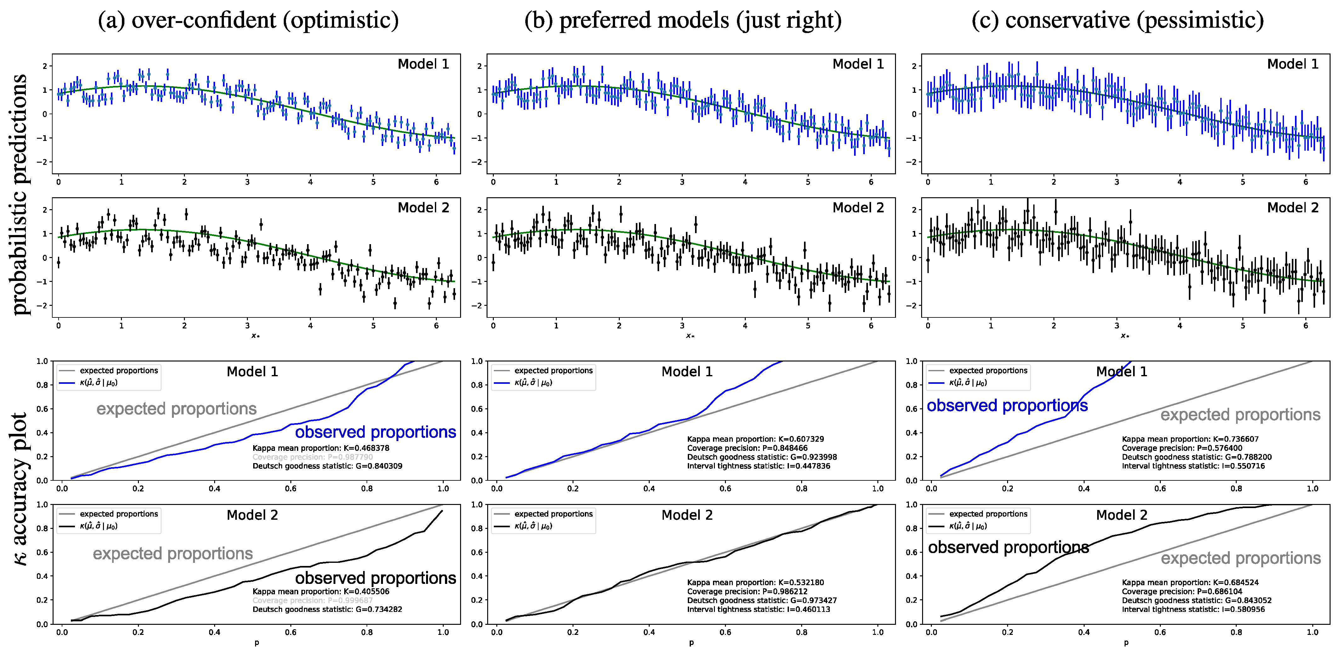
Figure 3.
Evaluating the uncertainty and predictive performance of two synthesised models. Top: probabilistic predictions. Bottom: accuracy plots. From left to right, (a–c) show what can be expected from the optimistic, preferred and conservative models.
Figure 3.
Evaluating the uncertainty and predictive performance of two synthesised models. Top: probabilistic predictions. Bottom: accuracy plots. From left to right, (a–c) show what can be expected from the optimistic, preferred and conservative models.
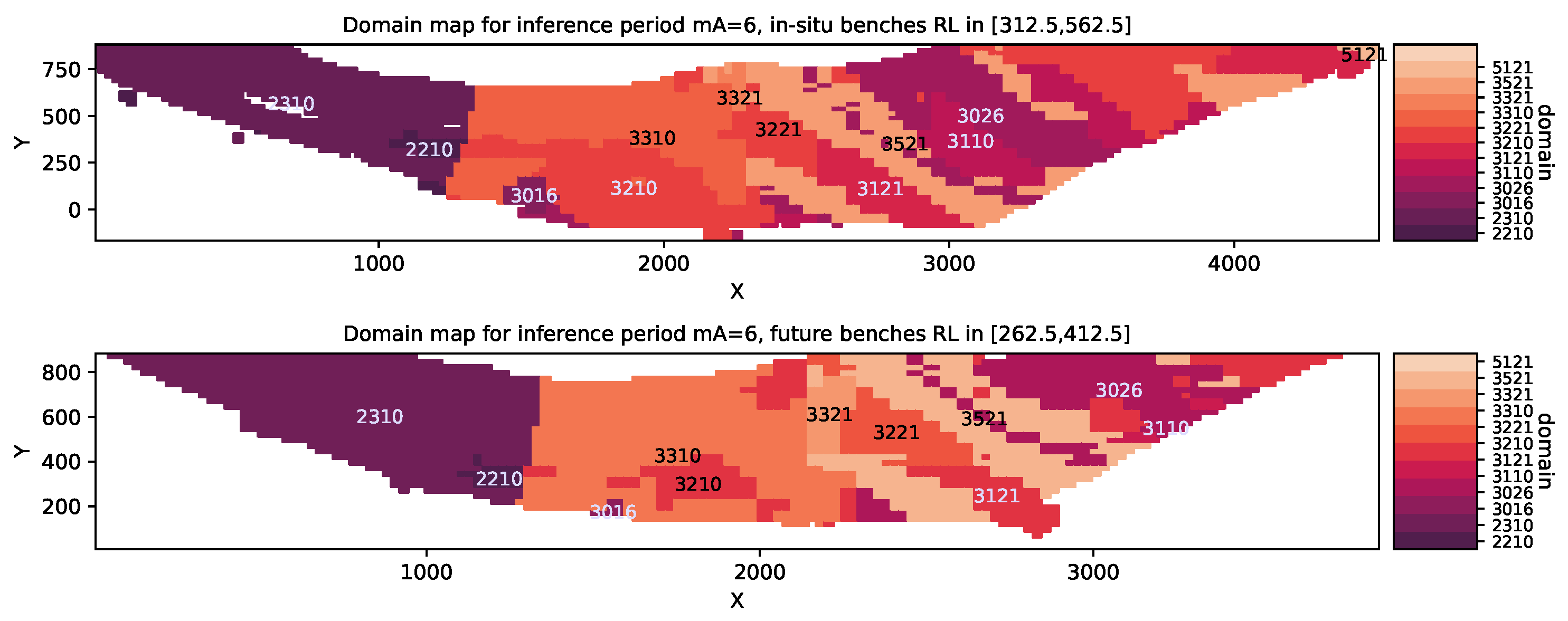
Figure 4.
The orebody is partitioned into different geological domains to facilitate copper grade modelling. The panels show correlated spatial structure and subtle changes at different RL elevations. Top image shows blocks associated with active mining operations, i.e., benches that may benefit from in situ regression. Bottom image shows blocks associated with future-bench prediction which require extrapolation. It should be noted that the actual spatial coordinates are shifted so that the minimum coordinates of the study area are close to the origin in the Cartesian coordinates system. This applies also to the RL elevation (ft) to anonymise the data due to commercial sensitivity.
Figure 5.
Copper grade distribution across different domains for inference period mA = 6. In each box-plot, the outer (faint) and inner (dark) whiskers represent the 2.15/97.85 and 8.87/91.13 percentiles, whereas the horizontal bar and box edges represent the median and lower/upper quartiles, respectively. From an economic perspective, porphyry orebodies can be mined profitably from Cu concentrations as low as 0.15–0.3%. The left, middle and right plots pertain to blasthole training data, blocks that require in situ regression and future-bench prediction, respectively. As expected, in situ distributions more closely resemble the training data than future-bench distributions.
Figure 6.
Visualisation of copper grade for blasthole training data (left) and ground truth at predicted locations (right) for two domains, 2310 (top) and 3521 (bottom), in inference period mA = 4.
Figure 6.
Visualisation of copper grade for blasthole training data (left) and ground truth at predicted locations (right) for two domains, 2310 (top) and 3521 (bottom), in inference period mA = 4.
Figure 7.
Mean copper grade predicted by models for domain gD = 2310 and inference period mA = 4.
Figure 7.
Mean copper grade predicted by models for domain gD = 2310 and inference period mA = 4.
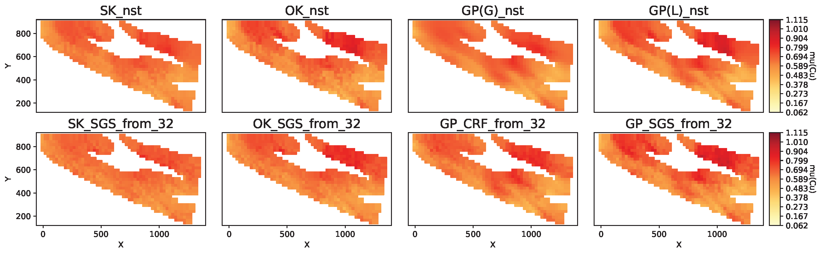
Figure 8.
Mean copper grade predicted by models for domain gD = 3521 and inference period mA = 4.
Figure 8.
Mean copper grade predicted by models for domain gD = 3521 and inference period mA = 4.
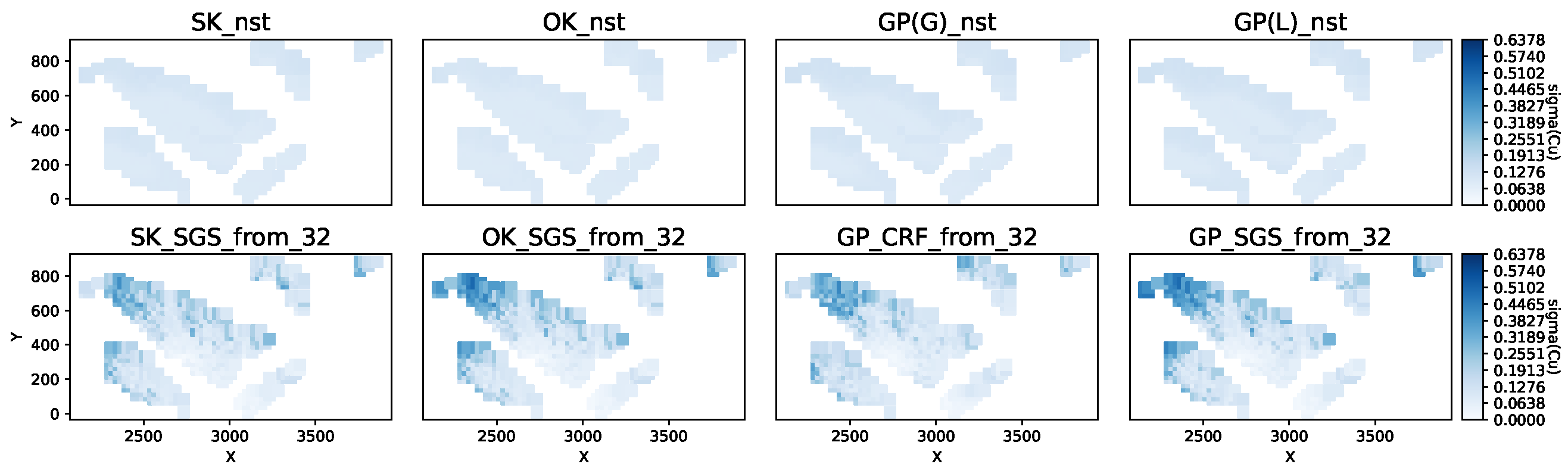
Figure 9.
Copper grade standard deviation predicted by models for domain gD = 2310 and inference period mA = 4.
Figure 9.
Copper grade standard deviation predicted by models for domain gD = 2310 and inference period mA = 4.
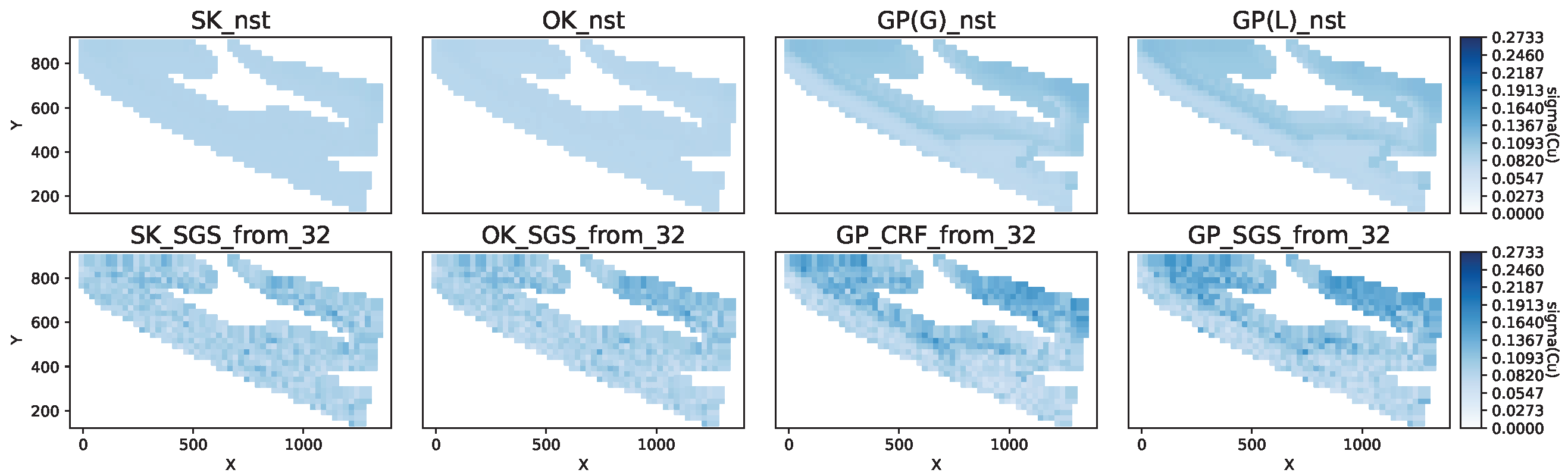
Figure 10.
Copper grade standard deviation predicted by models for domain gD = 3521 and inference period mA = 4.
Figure 10.
Copper grade standard deviation predicted by models for domain gD = 3521 and inference period mA = 4.
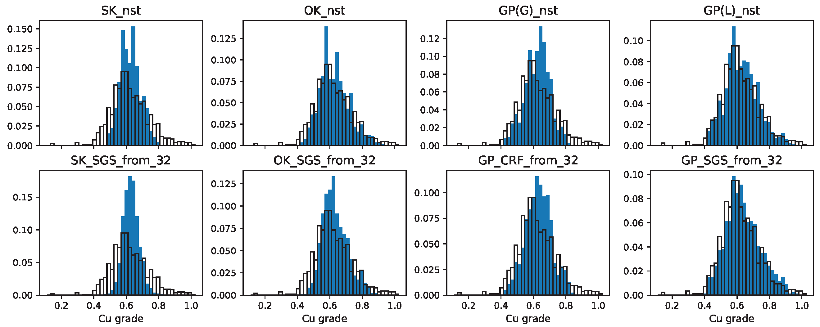
Figure 11.
Copper grade histograms for gD = 2310 and mA = 4. Black hollow: ground truth. Blue: model predictions.
Figure 11.
Copper grade histograms for gD = 2310 and mA = 4. Black hollow: ground truth. Blue: model predictions.
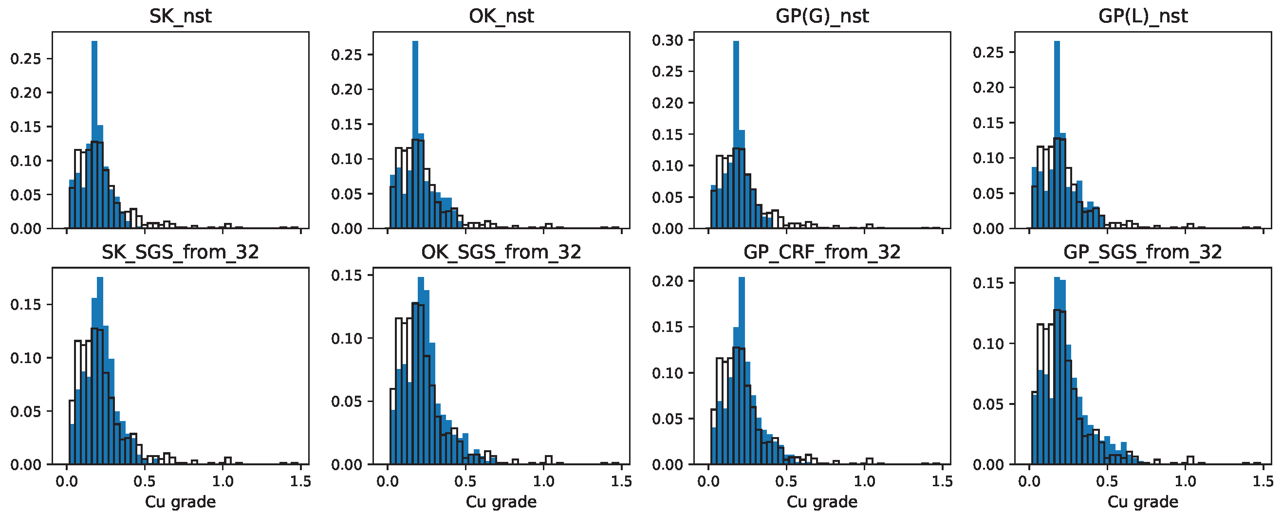
Figure 12.
Copper grade histograms for gD = 3521 and mA = 4. Black hollow: ground truth. Blue: model predictions.
Figure 12.
Copper grade histograms for gD = 3521 and mA = 4. Black hollow: ground truth. Blue: model predictions.
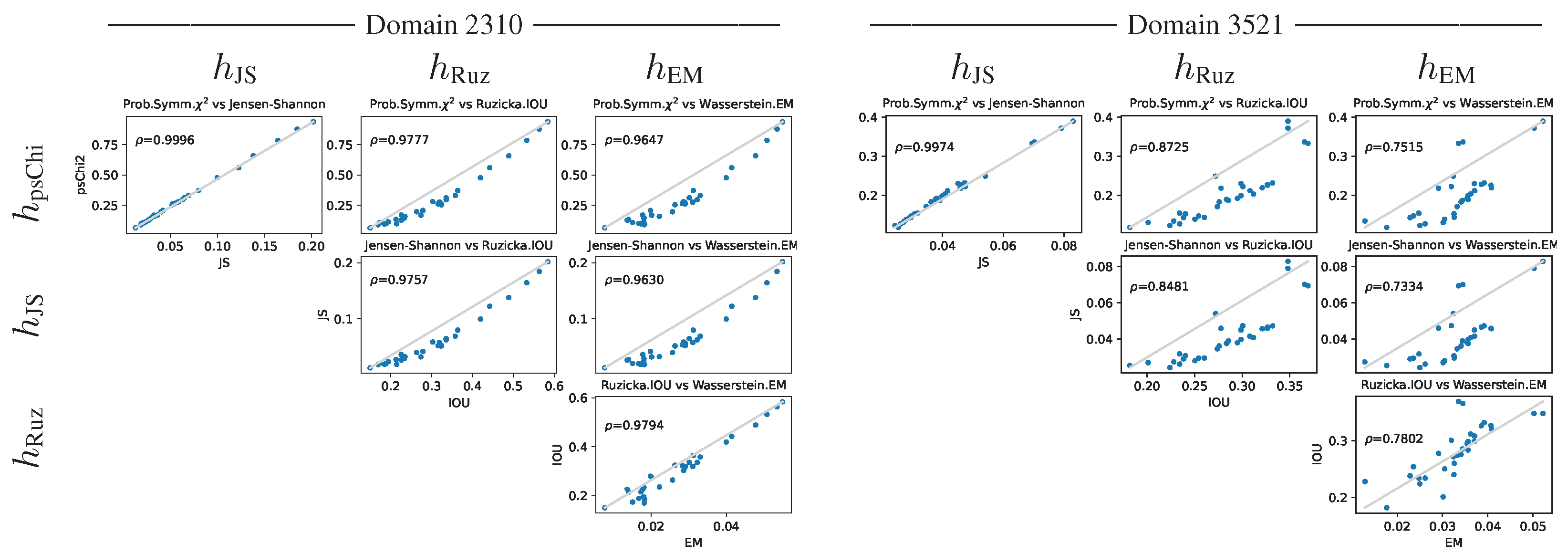
Figure 13.
Histogram distances cross-plots for gD = 2310 and gD = 3521 in mA = 4.
Figure 13.
Histogram distances cross-plots for gD = 2310 and gD = 3521 in mA = 4.
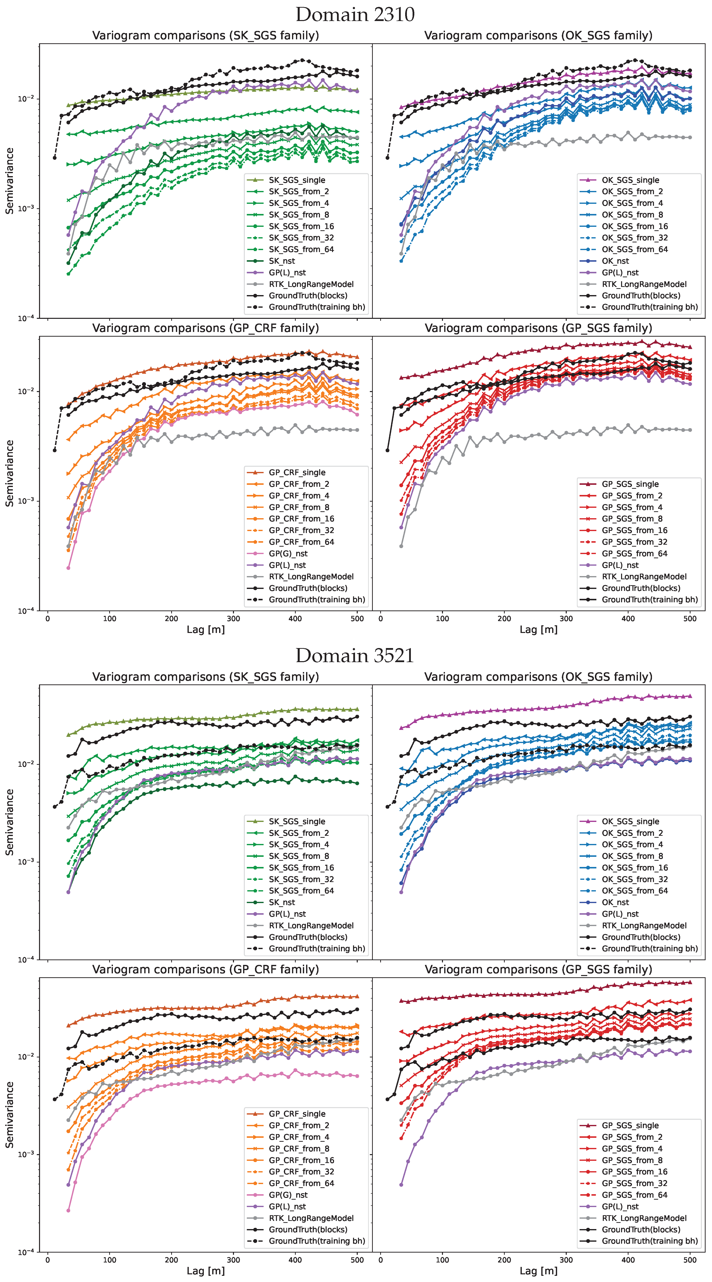
Figure 14.
Copper grade variograms for gD = 2310 and gD = 3521 in mA = 4. The quadrants group together models in the following families: (northwest) SK/SK-SGS, (northeast) OK/OK-SGS, (southwest) GP(G)/GP-CRF, (southeast) GP(L)/GP-SGS.
Figure 14.
Copper grade variograms for gD = 2310 and gD = 3521 in mA = 4. The quadrants group together models in the following families: (northwest) SK/SK-SGS, (northeast) OK/OK-SGS, (southwest) GP(G)/GP-CRF, (southeast) GP(L)/GP-SGS.
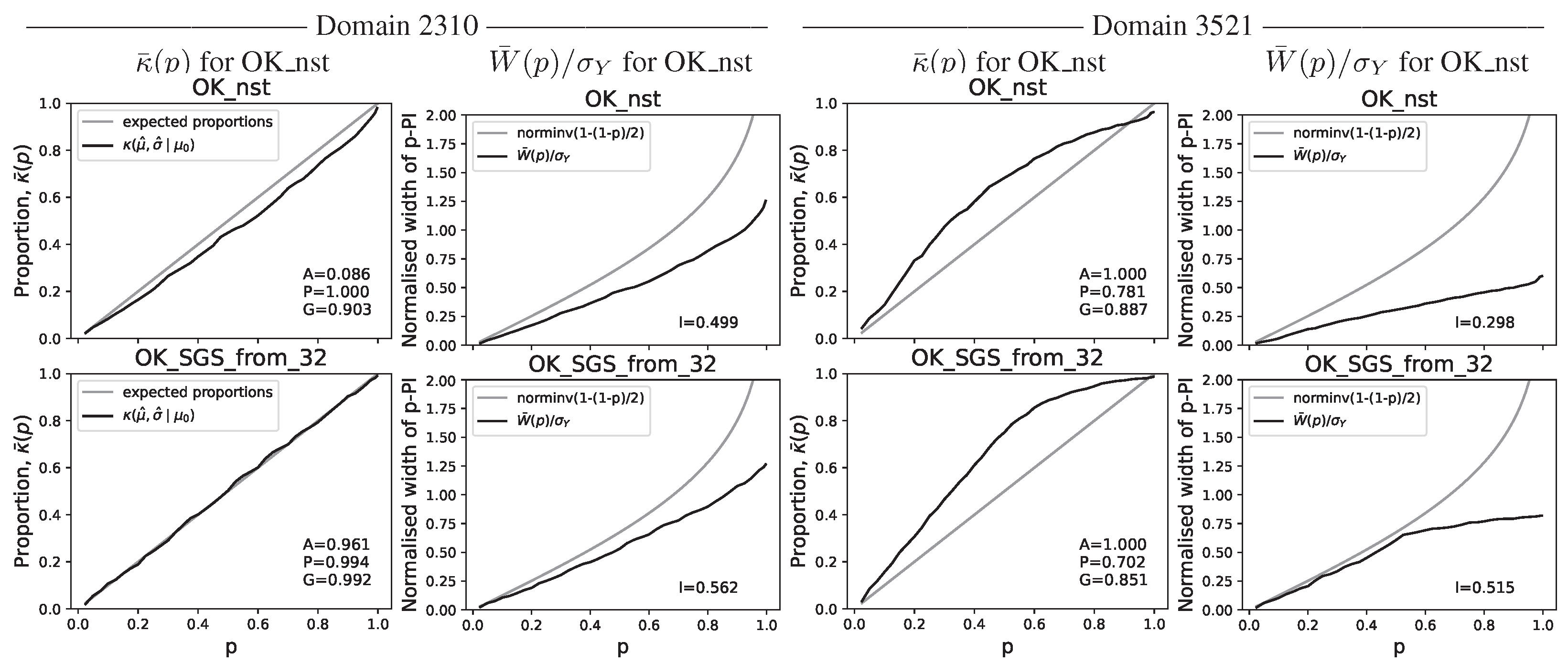
Figure 15.
Copper grade predictive distribution accuracy and uncertainty interval plots. Selected results for gD = 2310 and gD = 3521 in mA = 4.
Figure 15.
Copper grade predictive distribution accuracy and uncertainty interval plots. Selected results for gD = 2310 and gD = 3521 in mA = 4.
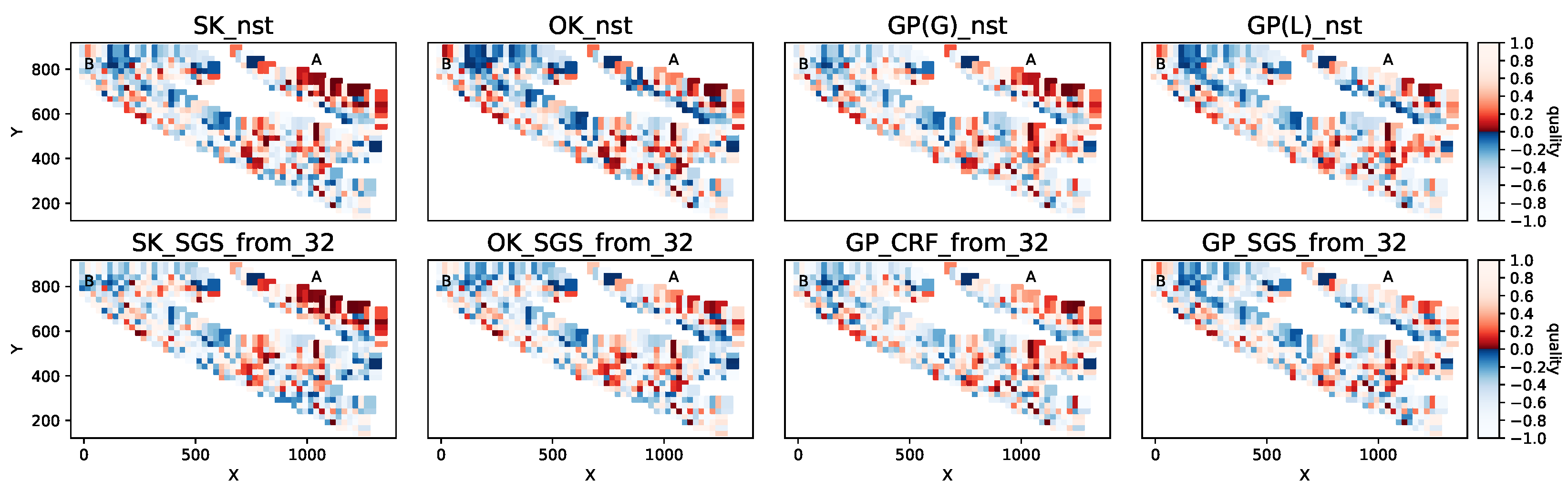
Figure 16.
Synchronicity of grade predictions with regard to the ground truth for gD = 2310 and mA = 4.
Figure 16.
Synchronicity of grade predictions with regard to the ground truth for gD = 2310 and mA = 4.
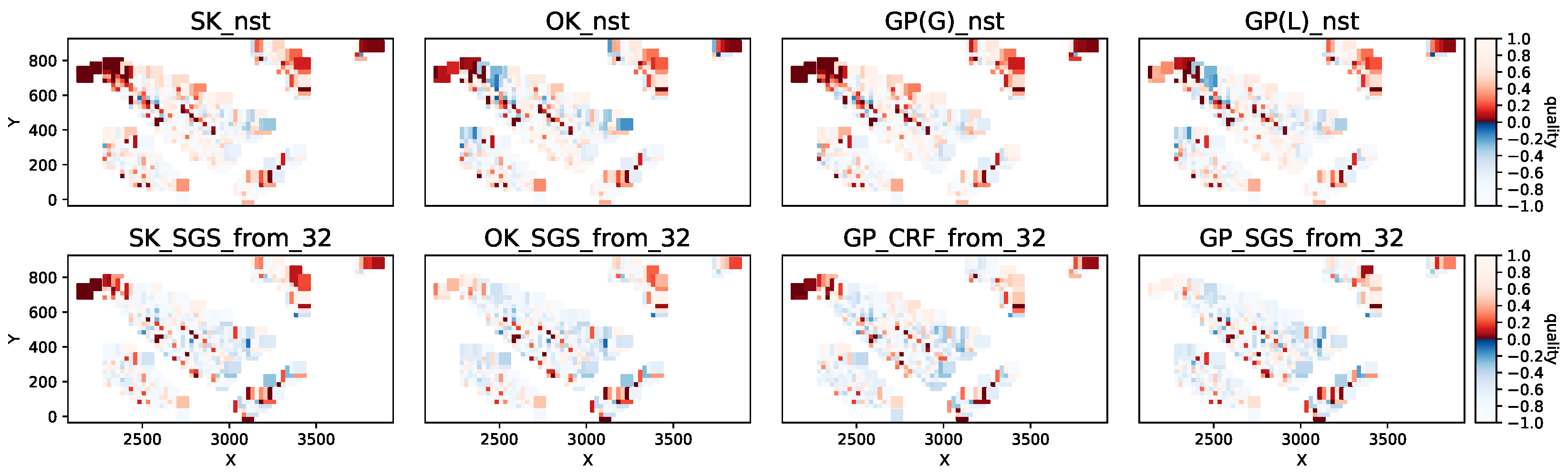
Figure 17.
Synchronicity of grade predictions with regard to the ground truth for gD = 3521 and mA = 4.
Figure 17.
Synchronicity of grade predictions with regard to the ground truth for gD = 3521 and mA = 4.
Figure 18.
View of (left) Jensen–Shannon and (right) EM histogram distances for future-bench prediction across domains and inference periods.
Figure 18.
View of (left) Jensen–Shannon and (right) EM histogram distances for future-bench prediction across domains and inference periods.
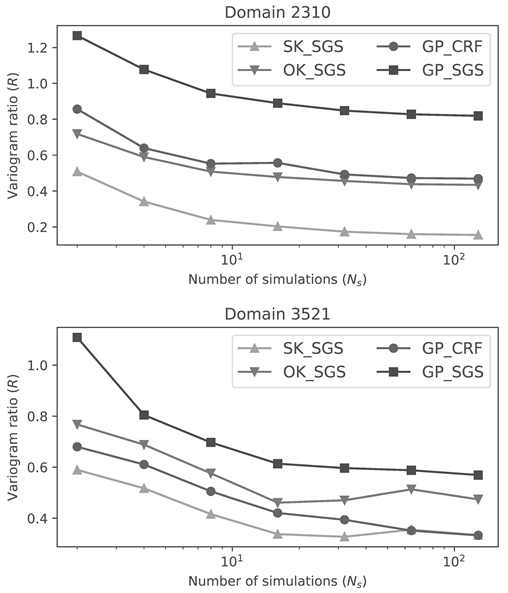
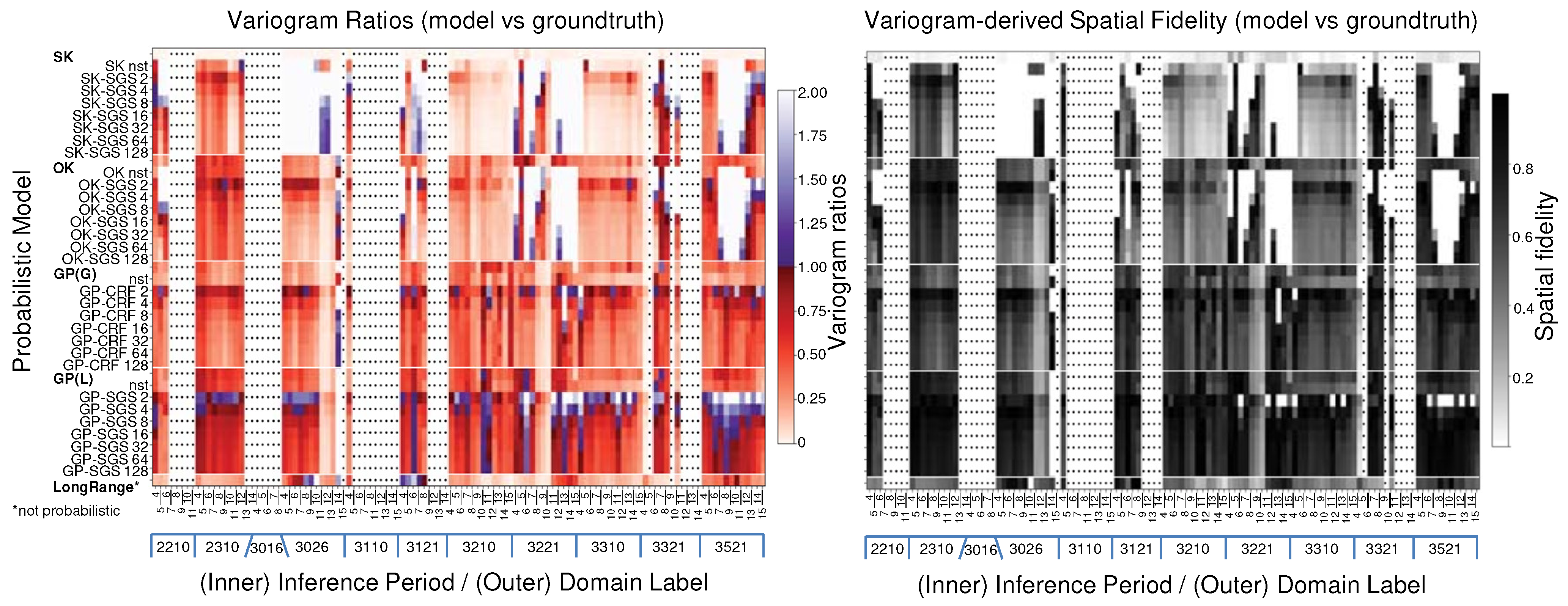
Figure 19.
View of (left) variogram ratios R and (right) spatial fidelity F for future-bench prediction across domains and inference periods.
Figure 19.
View of (left) variogram ratios R and (right) spatial fidelity F for future-bench prediction across domains and inference periods.
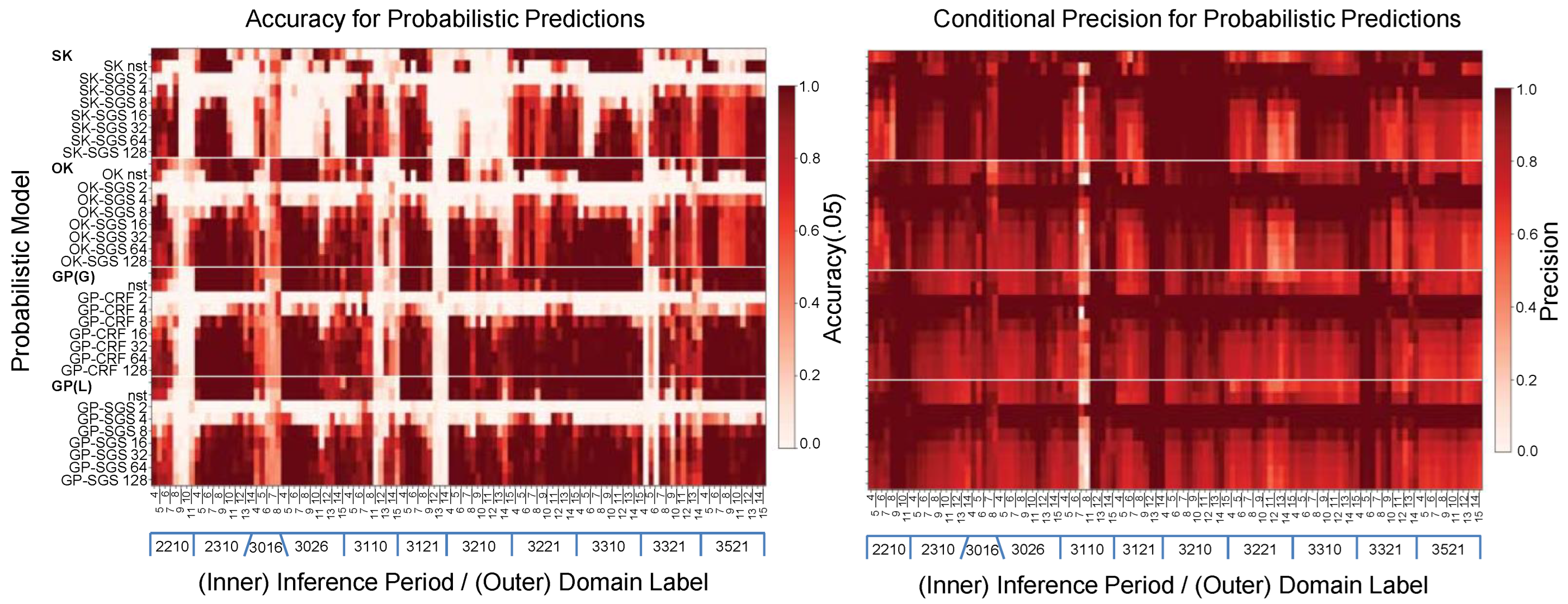
Figure 20.
View of (left) accuracy A and (right) precision P for future-bench prediction across domains and inference periods.
Figure 20.
View of (left) accuracy A and (right) precision P for future-bench prediction across domains and inference periods.
Figure 21.
View of (left) consensus L and (right) goodness G for future-bench prediction across domains and inference periods.
Figure 21.
View of (left) consensus L and (right) goodness G for future-bench prediction across domains and inference periods.
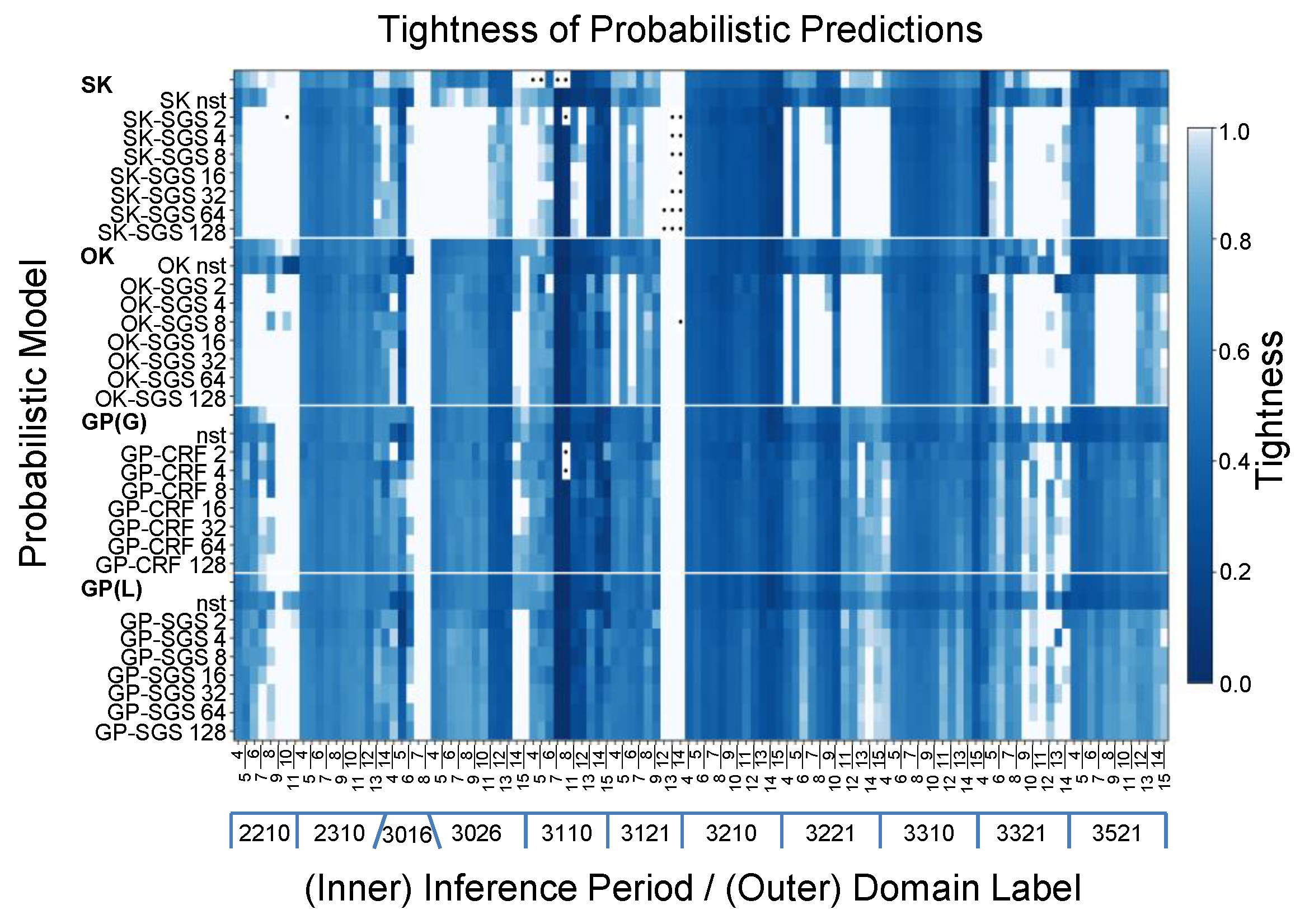
Figure 22.
View of interval tightness I for future-bench prediction across domains and inference periods.
Figure 22.
View of interval tightness I for future-bench prediction across domains and inference periods.
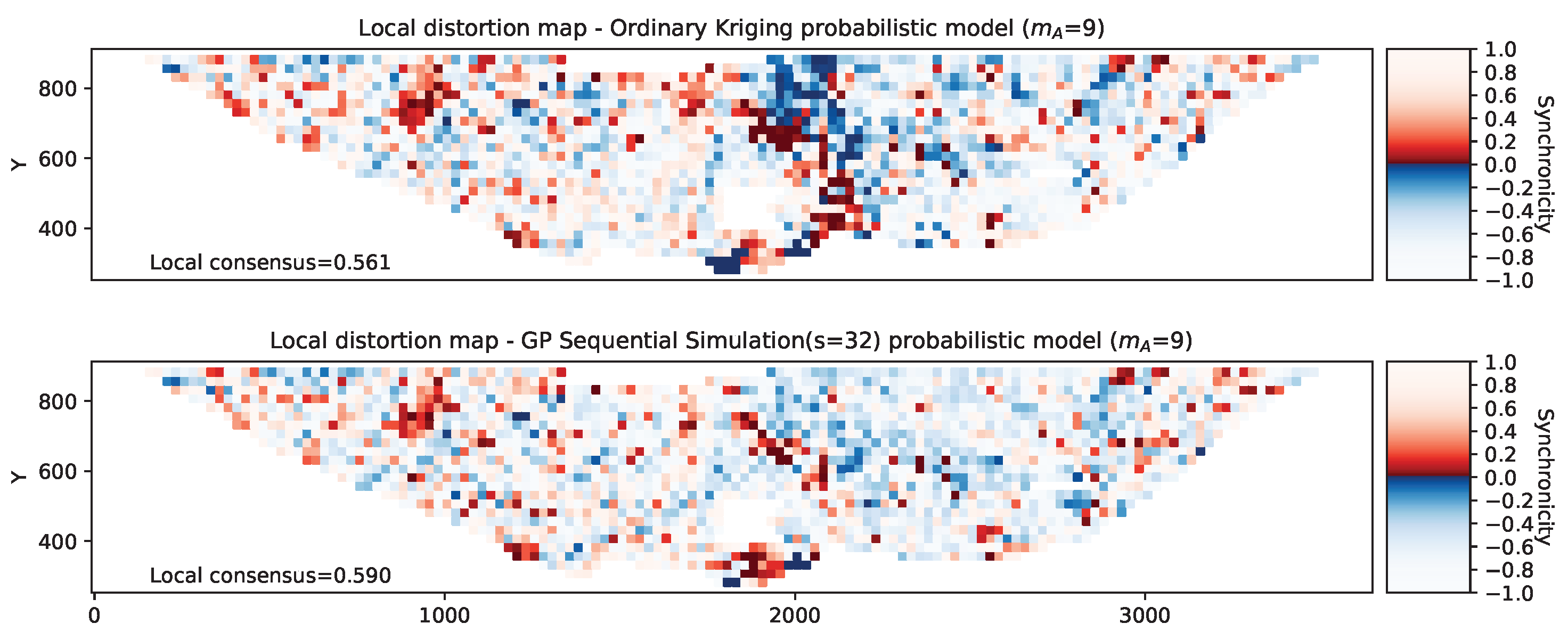
Figure 23.
Synchronicity map comparing model predictions with the ground truth across multiple domains. Dark patches indicate a high degree of inconsistency between prediction and ground truth. Red and blue colours indicate underestimation and overestimation, respectively.
Figure 23.
Synchronicity map comparing model predictions with the ground truth across multiple domains. Dark patches indicate a high degree of inconsistency between prediction and ground truth. Red and blue colours indicate underestimation and overestimation, respectively.
Table 1.
Model candidates for probabilistic copper grade estimation.
Table 1.
Model candidates for probabilistic copper grade estimation.
Table 2.
Uncertainty-based statistics for the example in
Figure 3.
Table 2.
Uncertainty-based statistics for the example in
Figure 3.
| Model | Setting | Distribution † | Bias | Amplitude † | Consensus (L) | Proportion (K) | Precision (P) | Goodness (G) | Tightness (I) |
|---|
| a.1 | optimistic | uniform | 0 | 0.15 | 0.430 | 0.468 | – | 0.840 | 0.336 |
| b.1 | preferred | uniform | 0 | 0.225 | 0.576 | 0.607 ↑ | 0.848 ✓ | 0.923 ↑ | 0.447 |
| c.1 | pessimistic | uniform | 0 | 0.35 | 0.711 | 0.736 ↑ | 0.576 ↓ | 0.788 ↓ | 0.550 |
| a.2 | optimistic | normal | −0.2 | 0.15 | 0.369 | 0.405 | – | 0.734 | 0.331 |
| b.2 | preferred | normal | −0.2 | 0.225 | 0.494 | 0.532 ↑ | 0.986 ✓ | 0.973 ↑ | 0.460 |
| c.2 | pessimistic | normal | −0.1 | 0.35 | 0.656 | 0.684 ↑ | 0.686 ↓ | 0.843 ↓ | 0.580 |
Table 3.
Sample size statistics for in situ interpolation and future-bench extrapolation.
Table 3.
Sample size statistics for in situ interpolation and future-bench extrapolation.
| | Number of Blasthole Samples for Training † | Number of Locations Requiring Prediction †,‡ |
|---|
| | In Situ | Future Bench | In Situ | Future Bench |
|---|
| Lower quartile | 133 | 481 | 96 | 26 |
| Median | 694 | 1112 | 680 | 138 |
| Upper quartile | 2338 | 2293 | 1968 | 401 |
| Total count ⋆ | 148,302 | 160,459 | 125,004 | 29,689 |
Table 4.
Analysis roadmap.
Table 4.
Analysis roadmap.
| Section | Objectives |
|---|
| 5.1 | Preliminary analysis to illustrate the spatial characteristics of copper grade model predictions in two domains. |
| 5.1.1 | - | Examine data diversity and correlation between histogram distance measures (global accuracy). |
| 5.1.2, 5.1.3 and 5.1.4 | - | Examine variogram ratios and differences between models (local accuracy/spatial variability). |
| 5.1.5 | - | Examine the accuracy and interval tightness of predictive distributions (-plots, calibration/uncertainty). |
| 5.1.6 | - | Use synchronicity measure to render local consensus/distortion maps to identify error clusters. |
| 5.2 | Comprehensive analysis across all domains and inference periods. Goals: (1) Demonstrate an approach that supports automated model assessment and meaningful comparison across different domains and configurations; (2) add layers to the analysis to provide a more complete understanding of different facets of model performance. |
| 5.2.1, 5.2.2, 5.2.3, 5.2.4, 5.2.5 and 5.2.6 | - | Introduce new assessment modality: image-based visualisation of standardised statistics. This focuses attention on instances where models underperform, whether by inspection or anomaly detection. |
| 5.2.7 and 5.2.8 | - | Compute confidence interval and test for statistical significance between models. |
| 5.3 | - | Measure the difficulty of future-bench prediction (extrapolation) relative to in situ regression (interpolation). |
| 5.4 | - | Consider the convergence and effects of sequential Gaussian simulations. |
| 6 | Discuss and reflect on the main features of the proposal and what it enables. |
Table 5.
Histogram distances for mean model predictions relative to ground truth.
Table 5.
Histogram distances for mean model predictions relative to ground truth.
| Model | Domain 2310 | Domain 3521 |
|---|
| | | | Rank | | | | | Rank |
|---|
| SK_nst | 0.5594 | 0.1225 | 0.4422 | 0.0414 | 7 | 0.3723 | 0.0791 | 0.3480 | 0.0502 | 7 |
| OK_nst | 0.2071 | 0.0422 | 0.2792 | 0.0199 | 3 | 0.3368 | 0.0702 | 0.3656 | 0.0345 | 6 |
| GP(L)_nst | 0.1273 | 0.0266 | 0.2261 | 0.0137 | 2 | 0.3335 | 0.0695 | 0.3690 | 0.0335 | 5 |
| GP(G)_nst | 0.3303 | 0.0693 | 0.3578 | 0.0331 | 6 | 0.3900 | 0.0829 | 0.3480 | 0.0522 | 8 |
| SK-SGS (from 32) | 0.8774 | 0.1845 | 0.5629 | 0.0535 | 8 | 0.2198 | 0.0458 | 0.3210 | 0.0408 | 4 |
| OK-SGS (from 32) | 0.3119 | 0.0650 | 0.3356 | 0.0302 | 5 | 0.1929 | 0.0380 | 0.2949 | 0.0354 | 3 |
| GP-SGS (from 32) | 0.0948 | 0.0192 | 0.1851 | 0.0182 | 1 | 0.1902 | 0.0376 | 0.2835 | 0.0357 | 2 |
| GP-CRF (from 32) | 0.2763 | 0.0580 | 0.3194 | 0.0311 | 4 | 0.1876 | 0.0391 | 0.2854 | 0.0344 | 1 |
Table 6.
Variogram ratios (R) and spatial fidelity (F) statistics for gD = 2310 and gD = 3521 in mA = 4.
Table 6.
Variogram ratios (R) and spatial fidelity (F) statistics for gD = 2310 and gD = 3521 in mA = 4.
| | Domain 2310 | Domain 3521 | ![Modelling 06 00050 i001]() |
| | | | | |
| SK_nst | 0.2775 | 0.5267 | 0.2328 | 0.4824 |
| OK_nst | 0.5945 | 0.7710 | 0.3311 | 0.5754 |
| GP(L)_nst | 0.7568 | 0.8699 | 0.3451 | 0.5874 |
| GP(G)_nst | 0.4525 | 0.6726 | 0.2217 | 0.4708 |
| SK-SGS (from 4) | 0.3415 | 0.5843 | 0.5171 | 0.7190 |
| OK-SGS (from 4) | 0.5894 | 0.7677 | 0.6882 | 0.8295 |
| GP-SGS (from 4) | 1.0774 | 0.9605 | 0.8046 | 0.8969 |
| GP-CRF (from 4) | 0.6391 | 0.7994 | 0.6105 | 0.7813 |
| SK-SGS (from 32) | 0.1736 | 0.3998 | 0.3275 | 0.5722 |
| OK-SGS (from 32) | 0.4565 | 0.6756 | 0.4705 | 0.6859 |
| GP-SGS (from 32) | 0.8481 | 0.9209 | 0.5964 | 0.7722 |
| GP-CRF (from 32) | 0.4929 | 0.7020 | 0.3941 | 0.6277 |
Table 7.
Uncertainty-based statistics for gD = 2310 and gD = 3521 in mA = 4. Specifically, L, A, P, G and I denote the local consensus, accuracy, precision, goodness and interval tightness of the probabilistic predictions.
Table 7.
Uncertainty-based statistics for gD = 2310 and gD = 3521 in mA = 4. Specifically, L, A, P, G and I denote the local consensus, accuracy, precision, goodness and interval tightness of the probabilistic predictions.
| | Domain 2310 | Domain 3521 |
|---|
| | | | | | | | | | | |
|---|
| SK_nst | 0.4817 | 0.6172 | 1.0000 | 0.9631 | 0.5182 | 0.6231 | 1.0000 | 0.7480 | 0.8686 | 0.2918 |
| OK_nst | 0.4517 | 0.0859 | 0.9999 | 0.9030 | 0.4992 | 0.6075 | 1.0000 | 0.7808 | 0.8866 | 0.2984 |
| GP(L)_nst | 0.4963 | 0.9062 | 0.9953 | 0.9857 | 0.5752 | 0.6353 | 1.0000 | 0.7272 | 0.8618 | 0.3071 |
| GP(G)_nst | 0.5184 | 1.0000 | 0.9628 | 0.9812 | 0.5548 | 0.6294 | 1.0000 | 0.7361 | 0.8634 | 0.2965 |
| SK-SGS (from 32) | 0.4967 | 0.9297 | 0.9987 | 0.9913 | 0.5652 | 0.6506 | 1.0000 | 0.6978 | 0.8484 | 0.4246 |
| OK-SGS (from 32) | 0.5010 | 0.9609 | 0.9936 | 0.9925 | 0.5617 | 0.6485 | 1.0000 | 0.7022 | 0.8509 | 0.5152 |
| GP-SGS (from 32) | 0.5071 | 0.7383 | 0.9753 | 0.9771 | 0.6531 | 0.6411 | 1.0000 | 0.7172 | 0.8585 | 0.5311 |
| GP-CRF (from 32) | 0.5265 | 0.9961 | 0.9462 | 0.9723 | 0.6208 | 0.6255 | 0.9727 | 0.7477 | 0.8730 | 0.4779 |
| ine SK-SGS (from 128) | 0.5116 | 0.9805 | 0.9754 | 0.9863 | 0.5659 | 0.6728 | 1.0000 | 0.6535 | 0.8266 | 0.4273 |
| OK-SGS (from 128) | 0.5142 | 0.9688 | 0.9707 | 0.9844 | 0.5661 | 0.6698 | 1.0000 | 0.6598 | 0.8298 | 0.5187 |
| GP-SGS (from 128) | 0.5232 | 0.9609 | 0.9530 | 0.9759 | 0.6475 | 0.6650 | 0.9961 | 0.6693 | 0.8346 | 0.5370 |
| GP-CRF (from 128) | 0.5434 | 1.0000 | 0.9127 | 0.9563 | 0.6085 | 0.6592 | 0.9961 | 0.6810 | 0.8404 | 0.4491 |
Table 8.
Histogram distance summary statistics for future-bench prediction over domains and inference periods.
Table 8.
Histogram distance summary statistics for future-bench prediction over domains and inference periods.
| Model Family | Abbrev | Mean | Mean |
|---|
| Simple kriging | SK/SK-SGS | 0.4607 | 0.1678 |
| Ordinary kriging | OK/OK-SGS | 0.3524 | 0.1126 |
| Gaussian process (global mean) | GP(G)/GP-CRF | 0.2937 | 0.0753 |
| Gaussian process (local mean) | GP(L)/GP-SGS | 0.2802 | 0.0691 |
Table 9.
Sample size statistics for certain domains (gD) and inference periods (mA) involved in future-bench prediction.
Table 9.
Sample size statistics for certain domains (gD) and inference periods (mA) involved in future-bench prediction.
| gD | mA | | | gD | mA | | | gD | mA | | | gD | mA | | | gD | mA | | |
|---|
| 2210 | 4 | 76 | 66 | | 10 | 123 | 5 | | 6 | 86 | 10 | | 15 | 2120 | 10 | | 9 | 208 | 28 |
| | 5 | 66 | 30 | | 11 | 123 | 4 | | 7 | 86 | 2 | 3321 | 4 | 14 | 49 | | 10 | 224 | 36 |
| | 6 | 114 | 37 | 2310 | 13 | 2653 | 19 | | 8 | 86 | 2 | | 5 | 61 | 101 | | 11 | 227 | 12 |
| | 7 | 109 | 16 | | 14 | 2654 | 19 | 3026 | 12 | 2050 | 111 | | 6 | 59 | 104 | | 12 | 242 | 16 |
| | 8 | 130 | 15 | 3016 | 4 | 67 | 28 | | 13 | 2088 | 75 | | 7 | 143 | 108 | | 13 | 238 | 4 |
| | 9 | 121 | 9 | | 5 | 81 | 8 | | 14 | 2113 | 35 | | 8 | 195 | 68 | | 14 | 242 | 4 |
Table 10.
Variogram ratio (R) and spatial fidelity (F) summary statistics for future-bench prediction over domains and inference periods.
Table 10.
Variogram ratio (R) and spatial fidelity (F) summary statistics for future-bench prediction over domains and inference periods.
| Model Family | Abbrev | R Mean (SE) | F Mean (SE) |
|---|
| Simple kriging | SK/SK-SGS | 0.2983 (0.0112) | 0.4272 (0.0125) |
| Ordinary kriging | OK/OK-SGS | 0.4787 (0.0102) | 0.6234 (0.0110) |
| Gaussian process (global mean) | GP(G)/GP-CRF | 0.6114 (0.0070) | 0.7675 (0.0055) |
| Gaussian process (local mean) | GP(L)/GP-SGS | 0.7132 (0.0081) | 0.8231 (0.0069) |
Table 11.
Accuracy (A) and precision (P) summary statistics for future-bench prediction over domains and inference periods.
Table 11.
Accuracy (A) and precision (P) summary statistics for future-bench prediction over domains and inference periods.
| Model Family | Abbrev | A Mean (SE) | P Mean (SE) |
|---|
| Simple kriging | SK/SK-SGS | 0.5245 (0.0159) | 0.8680 (0.0058) |
| Ordinary kriging | OK/OK-SGS | 0.7173 (0.0133) | 0.8672 (0.0050) |
| Gaussian process (global mean) | GP(G)/GP-CRF | 0.8084 (0.0119) | 0.8637 (0.0041) |
| Gaussian process (local mean) | GP(L)/GP-SGS | 0.8127 (0.0117) | 0.8510 (0.0048) |
Table 12.
Consensus (L) and goodness (G) summary statistics for future-bench prediction over domains and inference periods.
Table 12.
Consensus (L) and goodness (G) summary statistics for future-bench prediction over domains and inference periods.
| Model Family | Abbrev | L Median | | G Mean (SE) |
|---|
| Simple kriging | SK/SK-SGS | 0.4527 | [0.2346, 0.6219] | 0.7149 (0.0076) |
| Ordinary kriging | OK/OK-SGS | 0.5137 | [0.2795, 0.6764] | 0.7868 (0.0065) |
| Gaussian process (global mean) | GP(G)/GP-CRF | 0.5366 | [0.2855, 0.6990] | 0.7974 (0.0062) |
| Gaussian process (local mean) | GP(L)/GP-SGS | 0.5432 | [0.2996, 0.7053] | 0.7997 (0.0059) |
Table 13.
Interval tightness (I) summary statistics for future-bench prediction over domains and inference periods.
Table 13.
Interval tightness (I) summary statistics for future-bench prediction over domains and inference periods.
| Model Family | Abbrev | I Mean (SE) |
|---|
| Simple kriging | SK/SK-SGS | 0.6898 (0.0096) |
| Ordinary kriging | OK/OK-SGS | 0.6408 (0.0087) |
| Gaussian process (global mean) | GP(G)/GP-CRF | 0.5787 (0.0072) |
| Gaussian process (local mean) | GP(L)/GP-SGS | 0.6180 (0.0073) |
Table 14.
Significance testing of statistical scores for future-bench prediction over all domains and inference periods.
Table 14.
Significance testing of statistical scores for future-bench prediction over all domains and inference periods.
| | Histogram | Spatial Fidelity F | Accuracy A | Precision P |
| Family | | CI | | CI | | CI | | CI |
| SK/SGS | <0.001 | | <0.001 | | <0.001 | | >0.99 | |
| OK/SGS | <0.001 | | <0.001 | | <0.001 | | >0.99 | |
| GP(G)/CRF | <0.001 | | <0.001 | | | | >0.95 | |
| Reference | | SE | | SE | | SE | | SE |
| GP(L)/SGS | | (0.0026) | 0.8231 | (0.0069) | 0.8127 | (0.0117) | 0.8510 | (0.0048) |
| | Interval I | Goodness | Consensus | |
| Family | | CI | | CI | p † | CI † | | |
| SK/SGS | <0.001 | | <0.001 | | <0.001 | | | |
| OK/SGS | <0.001 | | <0.001 | | | | | |
| GP(G)/CRF | >0.99 | | | | | | | |
| Reference | | SE | | SE | median | [] | | |
| GP(L)/SGS | 0.6180 | (0.0073) | 0.7997 | (0.0059) | 0.5432 | | | |
Table 15.
Performance comparison with in situ regression. Statistical scores for in situ regression are shown. Parentheses show percentage change as a general improvement relative to future-bench prediction. Note: The increase in difficulty going from in situ regression to future-bench prediction is given by . Figures are aggregated over all domains and inference periods.
| Family | Histogram | | Spatial Fidelity F | Accuracy A | Precision P | Interval I | Goodness G | Consensus L |
|---|
| SK/SGS | 0.1186 | (−29.3%) | 0.5149 | (+20.5%) | 0.6142 | (+17.1%) | 0.8840 † | (+1.84%) | 0.6964 | – | 0.7876 | (+10.1%) | 0.4731 | (+4.50%) |
| OK/SGS | 0.0790 | (−29.8%) | 0.7175 | (+15.0%) | 0.9051 | (+26.1%) | 0.8310 | (−4.17%) | 0.5924 | (−7.55%) | 0.8407 | (+6.85%) | 0.5708 | (+11.1%) |
| GP(G)/CRF | 0.0409 | (−45.6%) | 0.8482 | (+10.5%) | 0.9666 | (+19.5%) | 0.8303 | (−3.86%) | 0.4402 | (−23.9%) | 0.8546 | (+7.17%) | 0.5853 | (+9.07%) |
| GP(L)/SGS | 0.0382 | (−44.7%) | 0.8656 | (+5.16%) | 0.9723 | (+19.6%) | 0.8109 | (−4.71%) | 0.4445 | (−28.0%) | 0.8487 | (+6.12%) | 0.5954 | (+9.60%) |
Table 16.
Sample-weighted performance statistics for future-bench prediction.
Table 16.
Sample-weighted performance statistics for future-bench prediction.
| Model | Histogram | Spatial Fidelity | Abs. Synchronicity | Consensus | Accuracy | Precision | Goodness | Interval |
|---|
| | | | | | | | |
|---|
| GP(G)_nst | 0.1260 | 0.4856 | 0.3930 | 0.8229 | 0.5892 | 0.9585 | 0.8111 | 0.8954 | 0.4675 |
| GP(G)_CRF_from_2 | 0.0557 | 0.8617 | 0.0009 | 0.5166 | 0.2795 | 0.0047 | 0.9999 | 0.5578 | 0.5170 |
| GP(G)_CRF_from_4 | 0.0658 | 0.7424 | 0.1343 | 0.7035 | 0.4317 | 0.1440 | 0.9983 | 0.8605 | 0.5508 |
| GP(G)_CRF_from_8 | 0.0796 | 0.6740 | 0.2748 | 0.7643 | 0.5138 | 0.8532 | 0.9481 | 0.9498 | 0.5693 |
| GP(G)_CRF_from_16 | 0.0904 | 0.6303 | 0.3495 | 0.7948 | 0.5608 | 0.9606 | 0.8708 | 0.9280 | 0.5658 |
| GP(G)_CRF_from_32 | 0.0990 | 0.6063 | 0.3931 | 0.8111 | 0.5866 | 0.9768 | 0.8211 | 0.9053 | 0.5687 |
| GP(G)_CRF_from_64 | 0.1052 | 0.5851 | 0.4170 | 0.8208 | 0.6020 | 0.9800 | 0.7909 | 0.8908 | 0.5631 |
| GP(G)_CRF_from_128 | 0.1094 | 0.5745 | 0.4297 | 0.8257 | 0.6103 | 0.9803 | 0.7748 | 0.8831 | 0.5615 |
| GP(L)_nst | 0.0896 | 0.6368 | 0.3935 | 0.8273 | 0.5933 | 0.9618 | 0.8032 | 0.8918 | 0.4748 |
| GP(L)_SGS_from_2 | 0.0576 | 0.8247 | 0.0012 | 0.5177 | 0.2811 | 0.0036 | 0.9999 | 0.5611 | 0.5814 |
| GP(L)_SGS_from_4 | 0.0579 | 0.8499 | 0.1504 | 0.7001 | 0.4369 | 0.1680 | 0.9980 | 0.8705 | 0.6202 |
| GP(L)_SGS_from_8 | 0.0606 | 0.8354 | 0.2909 | 0.7622 | 0.5208 | 0.8662 | 0.9382 | 0.9490 | 0.6323 |
| GP(L)_SGS_from_16 | 0.0687 | 0.8105 | 0.3651 | 0.7915 | 0.5665 | 0.9533 | 0.8596 | 0.9226 | 0.6372 |
| GP(L)_SGS_from_32 | 0.0732 | 0.7924 | 0.4065 | 0.8066 | 0.5914 | 0.9653 | 0.8116 | 0.9006 | 0.6404 |
| GP(L)_SGS_from_64 | 0.0793 | 0.7791 | 0.4304 | 0.8137 | 0.6067 | 0.9741 | 0.7820 | 0.8866 | 0.6426 |
| GP(L)_SGS_from_128 | 0.0815 | 0.7718 | 0.4454 | 0.8197 | 0.6153 | 0.9781 | 0.7651 | 0.8786 | 0.6417 |
Table 17.
EUP3M recommendations for evaluating the uncertainty and predictive performance of probabilistic models.
Table 17.
EUP3M recommendations for evaluating the uncertainty and predictive performance of probabilistic models.
| Material | Obtain a sufficiently large dataset with target attribute diversity to minimise selection bias and challenge the models. | Section 4.2 |
| Design | Experiments should reflect observational and modelling constraints in practice. For instance, the data available in each inference period defines the scope of our regression/prediction tasks in a manner that emulates staged data acquisition and progression of mining activities in a real mine. | Section 4.3 |
| Measures | Employ representative measures (such as the FLAGSHIP statistics) to investigate the global accuracy, local correlation and uncertainty-based properties of the models relative to the ground truth. [FLAGSHIP considers the spatial fidelity, local consensus, accuracy, goodness, synchronicity, histogram distance, interval tightness and precision of the predictive distributions.] | Section 3.1, Section 3.2, 3.3.1, 3.3.2, 3.3.3, 3.3.4, 3.3.5 and 3.3.6, (2)–(18) |
| Analysis | Perform one or more of the following according to needs: | |
| | (a) | Compute summary statistics to assess group performance: e.g., aggregate values by model family, average over domains or time periods (see Table 8, Table 9, Table 10, Table 11, Table 12 and Table 13). | Section 5.2.1, Section 5.2.2, Section 5.2.3, Section 5.2.4, Section 5.2.5 and Section 5.2.6 |
| | (b) | Observe general trends and variation in individual models: Perform large-scale simultaneous comparison across models and conditions using image-based views of the relevant statistics to identify instances where models may have underperformed (see Figure 18 and Figure 19). | Section 5.2 |
| | (c) | Establish statistical significance and confidence interval: e.g., perform hypothesis testing using t-tests and interpret the results using p-values and CIs. | Section 5.2.7 and Section 5.2.8 |
| | (d) | Contextualise model performance: e.g., compare in situ regression with future-bench prediction to articulate the difficulty of extrapolation relative to interpolation. Pairwise comparison can also reveal the benefits of modelling with additional data. | Section 5.3 |


