Machine Learning Models for Carbonation Depth Prediction in Reinforced Concrete Structures: A Comparative Study

Abstract

The durability of reinforced concrete (RC) structures is strongly influenced by carbonation, a phenomenon governed by material and environmental interactions. This study applied machine learning (ML) techniques—Random Forest (RF), Support Vector Regression (SVR), and Artificial Neural Networks (ANNs)—to predict carbonation depth using a synthetic dataset of 20,000 instances generated from the validated Possan equation. Model performances were evaluated across multiple scenarios, with compressive strength and exposure time identified as the most influential features, while relative humidity and exposure conditions had intermediate effects. SVR consistently captured linear and nonlinear trends, the ANN achieved the highest R² values but showed minor overestimations, and RF exhibited lower adaptability to feature variations. The results highlight the applicability of ML models for durability assessments, particularly under complex conditions where traditional approaches are limited. Moreover, this study reinforces the strategic value of synthetic datasets in developing predictive models when experimental data collection is time-consuming or impractical. The methodologies developed here can be extended beyond carbonation modeling to other deterioration processes, supporting data-driven strategies for maintenance planning and resilience design in RC structures.

1. Introduction

Carbonation is a chemical process in which atmospheric carbon dioxide (CO₂) penetrates concrete pores, dissolves in the pore water, and reacts with calcium hydroxide [Ca(OH)₂], forming calcium carbonate (CaCO₃) and lowering the pH of the material. This reduction in alkalinity compromises the passive layer of reinforcement steel, triggering corrosion processes and affecting the durability and service life of reinforced concrete (RC) structures [1,2,3]. With rising global CO₂ emissions, carbonation-induced deterioration is expected to accelerate, requiring more effective strategies for long-term durability prediction [4].

Several material and environmental factors influence carbonation depth in concrete. On the material side, parameters such as compressive strength, the water-to-cement ratio (w/c), the type of cement, the use of supplementary cementitious materials, and concrete cover thickness play a significant role. Environmentally, atmospheric CO₂ concentration, relative humidity, temperature, and exposure conditions (e.g., wetting–drying cycles) are critical to the advancement of the carbonation front [5,6,7,8].

Given these factors’ complexity and nonlinear interaction, machine learning (ML) techniques have emerged as promising tools for predicting carbonation depth in RC structures. ML models such as Artificial Neural Networks (ANNs), Support Vector Regression (SVR), and Random Forest (RF) have demonstrated effectiveness in capturing complex patterns and nonlinearities [9,10,11]. However, the “black box” nature of ML models often limits the adoption of these techniques, which hinders their interpretability [12,13].

In this context, the main contribution of this research is not limited to carbonation modeling but lies in the advancement of ML applications for complex degradation phenomena. The methods developed are highly generalizable and can be extended to a wide variety of durability-related problems across civil and materials engineering.

Explainable artificial intelligence (XAI) techniques, particularly SHapley Additive exPlanations (SHAP), have gained traction in addressing the interpretability limitations of ML models by enabling the attribution of importance values to each input feature based on its contribution to a specific prediction, thus enhancing model transparency and reliability [14,15,16]. Beyond carbonation prediction, SHAP has been successfully applied to estimate other durability-related properties, such as compressive strength, chloride diffusion, and wear depth in concrete [17,18,19]. It is important to note that although SHAP is acknowledged as a promising explainability tool in the context of ML models for carbonation prediction, the present study focuses exclusively on the comparative assessment of ML models’ predictive performance. The application of SHAP-based explainability will be explored in future studies.

Another major challenge in carbonation modeling is the limited availability of robust experimental datasets, especially under natural carbonation conditions. Accelerated carbonation tests often result in biased data distributions with low variability, limiting the generalization capabilities of ML models. To overcome this limitation, the present study adopts a synthetic dataset from the Possan equation [20], which was previously validated against natural and accelerated carbonation tests. Although synthetic datasets have inherent limitations, they enable the controlled exploration of a wide range of parameters and provide a valuable platform for methodological advancements in ML applications [21].

Thus, the key contributions of this study can be summarized as follows: (i) the development of a large synthetic dataset comprising 20,000 instances generated from the Possan equation, enabling a wide exploration of material and environmental conditions; (ii) the application and comparative evaluation of three ML models (RF, SVR, and ANN) for predicting carbonation depth in reinforced concrete structures; (iii) the execution of a feature behavior analysis to assess each model’s sensitivity to variations in key input parameters; and (iv) the demonstration of the strategic value of synthetic datasets for advancing ML-based durability assessments, especially in contexts where the collection of real-world experimental data is time-consuming, expensive, or impractical.

Hence, the main contribution of this study is methodological, focusing on developing and applying a synthetic dataset to evaluate the performance and behavior of established ML models in carbonation depth prediction rather than proposing new algorithms. Moreover, the methodology adopted herein is generic. It can be replicated to support ML applications in other civil engineering problems involving complex degradation mechanisms or scenarios where experimental data are scarce.

Research Problem, Related Works, and Main Definitions

Predicting carbonation depth in RC structures presents significant challenges due to the complexity of influencing factors and the scarcity of comprehensive datasets. This study conducts a comparative analysis of different ML techniques—RF, SVR, and ANNs—to identify the most efficient approach. A synthetic dataset containing 20,000 instances was developed to address traditional experimental datasets’ limitations and provide a robust platform for model evaluation.

Several studies have highlighted the application of ML techniques for predicting carbonation depth. Decision tree (DT)-based models were proposed by Taffese et al. [22], Nunez and Nehdi [23], Tran et al. [24], Londhe et al. [25], Huo et al. [26], Majlesi et al. [27], and Ehsani et al. [28]. ANN-based models were developed by Taffese et al. [22], Lee et al. [29], Uwanuakwa [30], Felix et al. [31], Chen et al. [32], Huo et al. [26], Majlesi et al. [27], Ehsani et al. [28], and Marani et al. [33]. Studies focusing on SVR were conducted by Uwanuakwa [30], Chen et al. [32], Huo et al. [26], Ehsani et al. [28], and Tran et al. [24].

ANNs have emerged as the most widely adopted and accurate technique for carbonation depth prediction [22,27,29,31], often outperforming alternative approaches. Hybrid models integrating ANNs with other techniques have also demonstrated superior results [26,32]. Tree-based models such as RF and Extreme Gradient Boosting (XGBoost) have proven robust and interpretable [23,24,25]. Although SVR generally exhibits slightly lower predictive accuracy than ANNs, it shows superior generalization capability across diverse scenarios [26,32].

Regarding dataset sources, most studies compiled data from the literature, frequently merging experimental results obtained under accelerated and natural carbonation conditions. This approach raises important methodological issues, as combining data from distinct carbonation environments can undermine the consistency and reliability of predictive models, leading to datasets with limited sizes and inherent biases (

Table 1. Dataset sizes reported in the literature.

Author(s)	Instances	Author(s)	Instances
Taffese et al. [22]	~184	Tran et al. [24]	688
Lee et al. [29]	206	Londhe et al. [25]	827
Uwanuakwa [30]	534	Huo et al. [26]	532
Nunez and Nehdi [23]	713	Majlesi et al. [27]	110
Felix et al. [31]	272	Ehsani et al. [28]	198
Chen et al. [32]	532	Marani et al. [33]	2165

). To date, no previous study has utilized a dataset as comprehensive and varied as the 20,000-instance synthetic dataset developed in the present research.

Inspired by the work of Martínez-Muñoz et al. [21], who effectively used synthetic datasets for structural optimization, this study demonstrates the significant advantages of synthetic data for expanding the analytical reach of ML models and covering broader carbonation scenarios.

The ML techniques considered include RF, SVR, and ANNs in this context. RF is an ensemble method that constructs multiple decision trees based on random subsets of the dataset. Each tree makes a prediction, and the RF aggregates these predictions by averaging them, enhancing accuracy and reducing the risk of overfitting [34,35,36,37], as illustrated in Figure 1.

SVR is an extension of the Support Vector Machine (SVM) algorithm for regression tasks. It aims to fit a function within a margin of tolerance (ε), ignoring minor errors within this range while minimizing model complexity [38,39,40,41]. A graphical representation of SVR for linear models is presented in Figure 2.

ANNs are computational models inspired by the human brain, consisting of interconnected layers of artificial neurons capable of learning complex and nonlinear patterns from data [41,42,43], as shown in Figure 3.

Thus, the main objective of this study is to perform a detailed and in-depth analysis of the impact of existing ML techniques on the prediction of carbonation depth. Specifically, this research seeks to (i) create and validate a robust synthetic dataset comprising 20,000 instances representing diverse environmental and material conditions; (ii) conduct a comparative analysis of different ML techniques—RF, SVR, and ANNs—highlighting their advantages and limitations; (iii) investigate the influence of individual features such as CO₂ concentration, compressive strength, relative humidity, the type of cement, exposure to rainfall, and time on carbonation progression; and (iv) identify under which conditions specific ML techniques outperform others, providing valuable insights for improving the assessment and service life evaluation of RC structures.

2. Materials and Methods

2.1. Dataset Generation

To address the inherent challenges in obtaining extensive real-world carbonation progression data within feasible timeframes, this study developed a synthetic dataset containing 20,000 instances. The dataset was generated using the Possan equation [20] (Equation (1)), a widely validated deterministic model that takes into consideration key factors influencing carbonation depth in concrete structures. Six input features were incorporated into the dataset: CO₂ concentration, concrete compressive strength, relative humidity, type of cement, exposure conditions, and time of exposure. These variables were randomly sampled within realistic ranges observed in reinforced concrete applications and environmental scenarios, ensuring a comprehensive and diversified parameter space. By enabling a controlled and systematic evaluation of ML models, the synthetic dataset overcomes limitations commonly associated with experimental data, such as restricted variability, small sample sizes, and non-random distributions. It is important to emphasize that the purpose of this dataset is not to explore new physical phenomena, but rather to provide a robust and unbiased platform for assessing the predictive performance of ML techniques in replicating known deterministic behaviors.

$$e_c=k_c\cdot ({\displaystyle \frac{20}{f_c}}{)}^{k_{\mathrm{fc}}}\cdot ({\displaystyle \frac{t}{20}}{)}^{{\displaystyle \frac{1}{2}}}\exp [({\displaystyle \frac{k_{\mathrm{ad}}{\mathrm{ad}}^{\frac{3}{2}}}{40+f_c}})+({\displaystyle \frac{k_{{\mathrm{CO}}_2}{{\mathrm{C}\mathrm{O}}_2}^{1/2}}{60+f_c}})-({\displaystyle \frac{k_{\mathrm{UR}}(\mathrm{UR}-0.58{)}^2}{100+f_c}})]\cdot k_{\mathrm{ce}}$$

(1)

In Equation (1), e_c represents the average carbonation depth (mm); f_c is the compressive strength of concrete (MPa); k_c is a factor related to the type of cement; k_fc is a factor associated with compressive strength, also dependent on cement type; t is the age of the concrete (years); ad is the percentage of pozzolanic addition relative to the cement mass; k_ad is a factor related to pozzolanic additions; UR is the average relative humidity (expressed as a fraction); k_UR is a factor linked to relative humidity, influenced by the type of cement; CO₂ is the atmospheric CO₂ concentration (%); k_CO2 is a factor accounting for CO₂ effects depending on cement; and k_ce is a factor related to rain exposure and the environmental conditions. The values of the coefficients (k_c, k_fc, k_ad, k_UR, k_CO2, and k_ce) are listed in

Table 2. Possan model coefficients related to concrete characteristics and environmental conditions [20].

Type of Cement	Concrete Characteristics			Environmental Conditions
	Cement	fc	Additions	CO2	UR
	kc	kfc	kad	kCO2	kUR
CP I	19.80	1.70	0.24	18.00	1300
CP II E	22.48	1.50	0.32	15.50	1300
CP II F	21.68	1.50	0.24	18.00	1100
CP II Z	23.66	1.50	0.32	15.50	1300
CP III	30.50	1.70	0.32	15.50	1300
CP IV	33.27	1.70	0.32	15.50	1000
CP V ARI	19.80	1.70	0.24	18.00	1300

and

Table 3. Possan model coefficients related to rain protection [20].

Exposure Condition	kce
Protected Indoor	1.30
Protected Outdoor	1.00
Unprotected Outdoor	0.65

[20]. Additional information regarding the types of cement and environmental conditions related to the coefficients presented in these tables is discussed in the subsequent paragraphs of this section.

The dataset was generated in Python v. 3.10 using the numpy library, specifically the numpy.random.uniform function to create random values within defined ranges.

Table 4. Features and corresponding ranges.

Feature	Adopted Values
CO2 Concentration (CCO2)	0.03–0.30%
Concrete Strength (fc)	20–50 MPa
Relative Humidity (UR) *	30–90%
Type of Cement	CPII E, CPII F, CPII Z, CPIII, CPIV, CPV-ARI
Exposure Conditions *	AIP, AEP, AED
Time (t)	0–100 years

Note: * Feature acronyms remain in Portuguese for consistency with the model variables.

summarizes the range for each variable considered, ensuring diversity and realism while minimizing potential biases. It is important to emphasize that the objective of this dataset is not to discover new physical phenomena but to evaluate the ML models’ ability to replicate known deterministic behaviors with high accuracy.

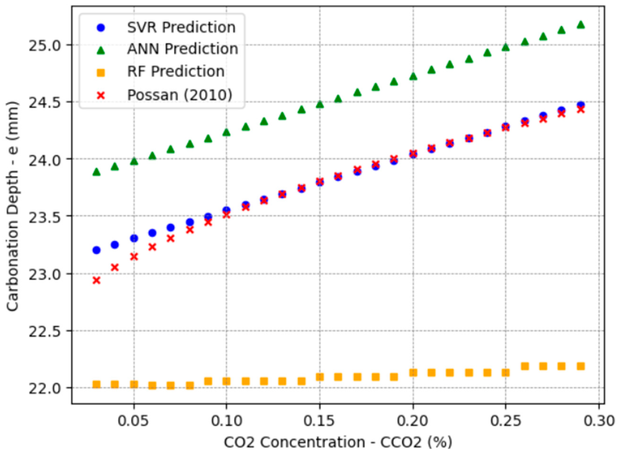
The CO₂ concentration range, from 0.03% to 0.30%, was selected based on values observed in various environments. Rural areas typically exhibit concentrations around 300 ppm (0.03%), whereas urban outdoor areas vary between 400 ppm (0.04%) and 500 ppm (0.05%) [44,45,46,47,48,49]. In enclosed environments within large cities, concentrations can reach 0.3% (3000 ppm), justifying the upper limit chosen. Although even higher concentrations can occur in poorly ventilated spaces such as garages, reaching up to 1% [46], the Possan equation mainly applies to typical urban conditions.

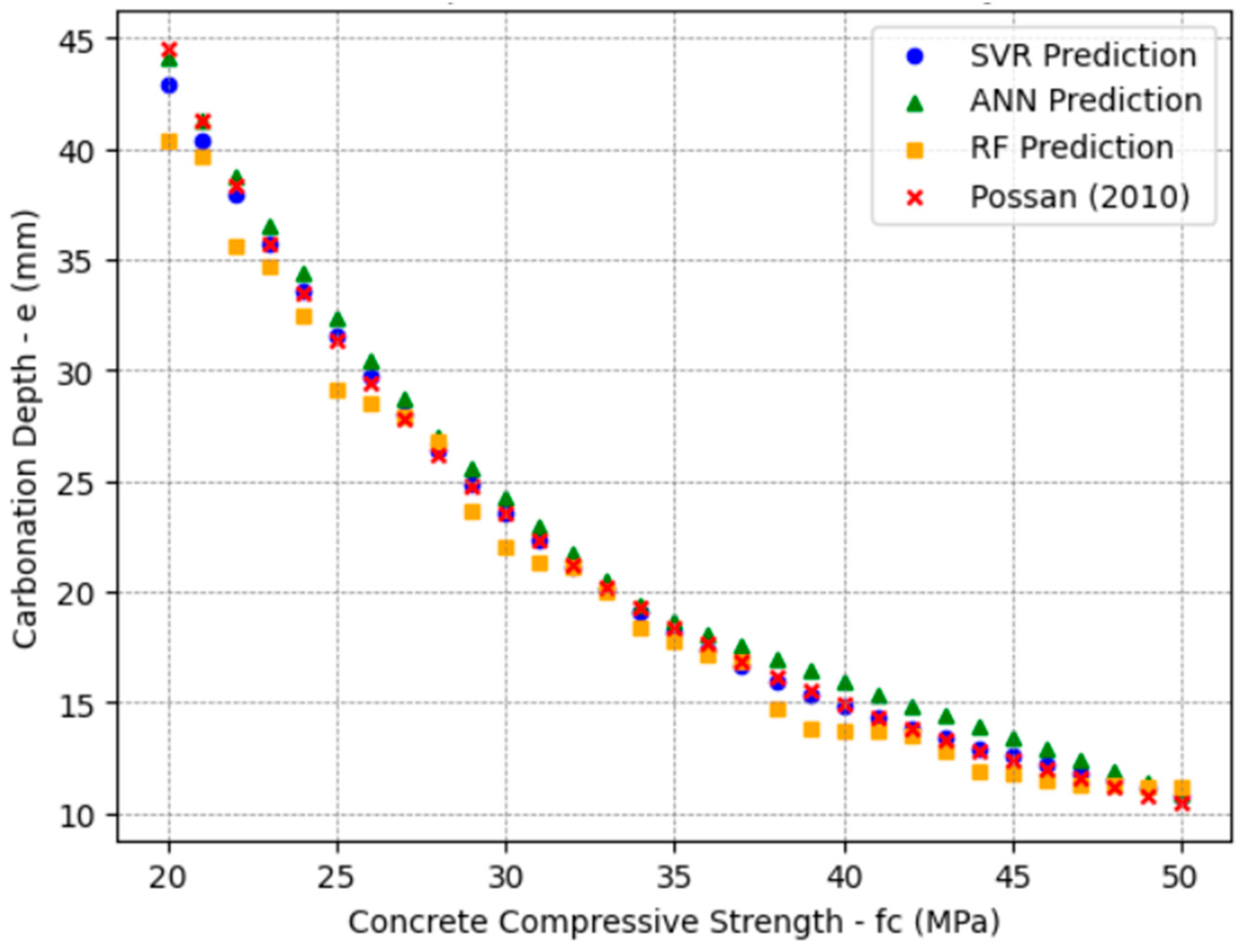
The adopted range (20–50 MPa) for concrete strength corresponds to Strength Class Group I concretes, as established by the Brazilian standard NBR 8953 [50]. The dataset was appropriately restricted because most existing RC structures fall within this group.

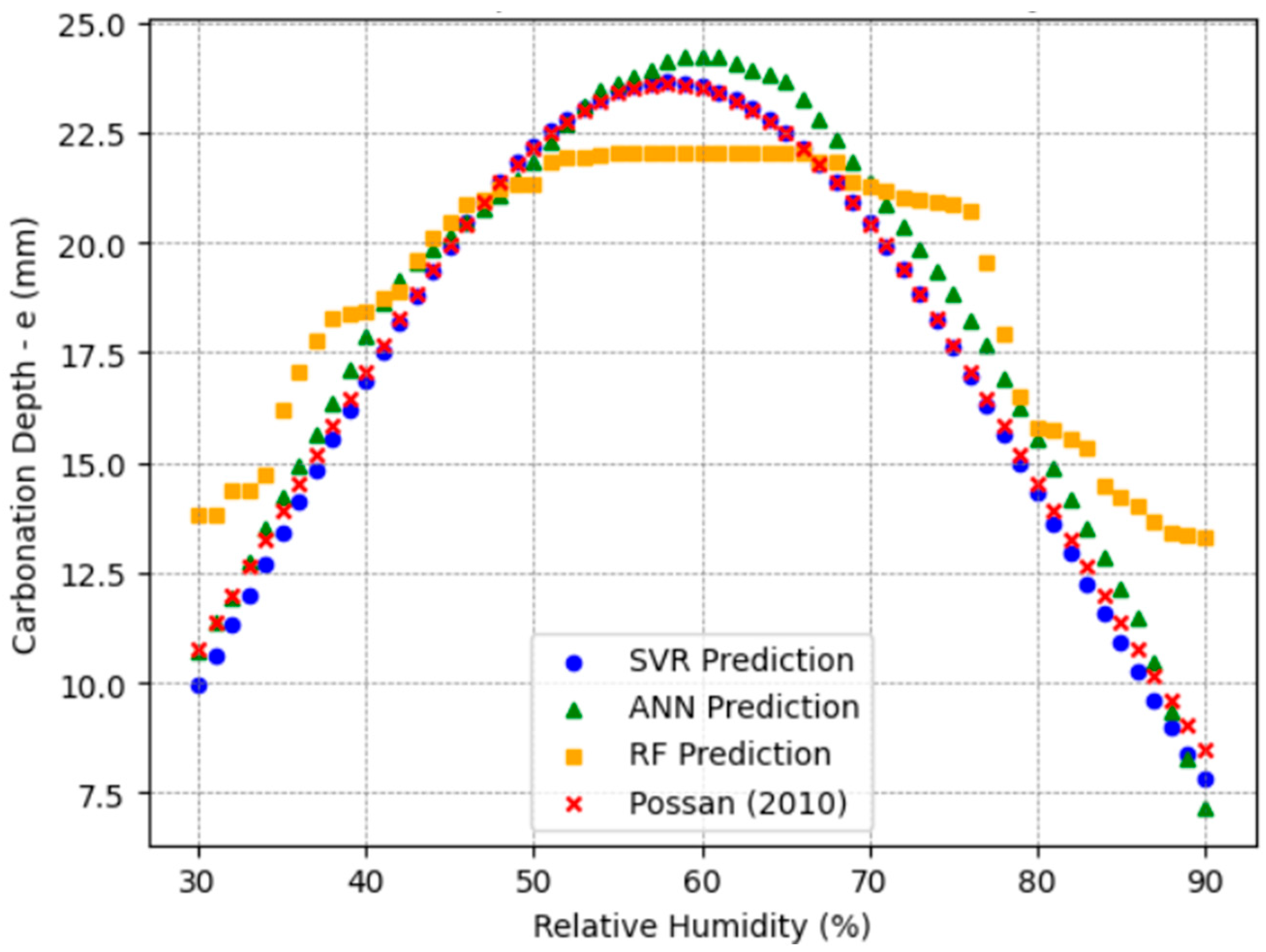
Regarding relative humidity, carbonation rapidly advances within the 50–70% range [20,46]. Thus, variations between 30% and 90% were considered to capture accelerated carbonation and protective effects caused by very low or very high humidity, reflecting global conditions.

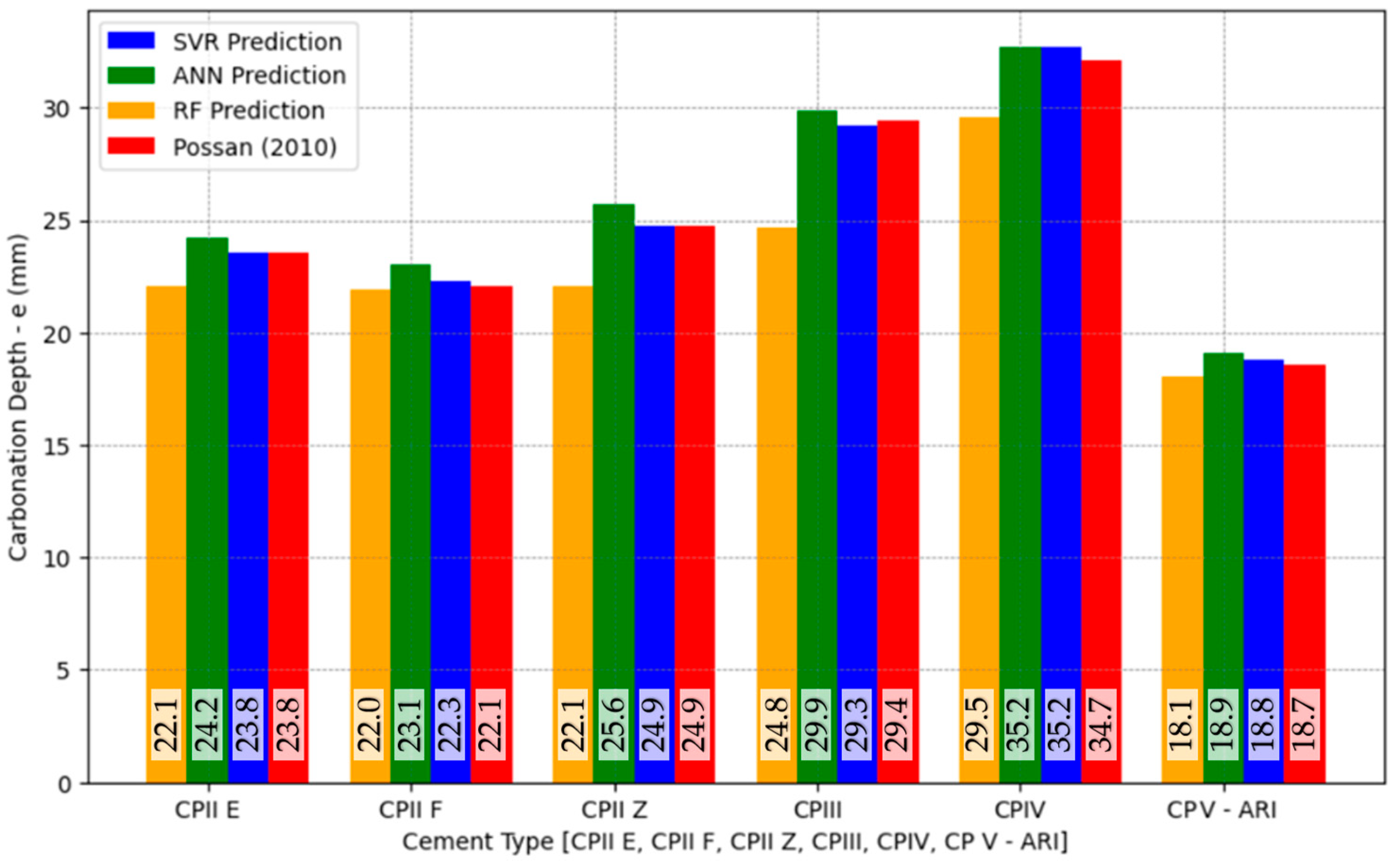
The approximate chemical compositions of the cement, based on typical formulations available in the Brazilian market and according to NBR 16697 [51], are as follows: CPII E contains about 70–80% clinker and 15–25% blast furnace slag; CPII F has approximately 70–80% clinker and 10–20% limestone filler; CPII Z comprises around 70–80% clinker and 15–25% pozzolanic materials; CPIII typically contains only 25–35% clinker and a high proportion of slag (60–70%); CPIV includes about 55–65% clinker and 25–40% pozzolans; and CPV-ARI is characterized by more than 90% clinker with minimal additions. These differences in clinker content are critical because carbonation resistance tends to decrease with lower clinker levels, as pozzolans and fillers generally provide less alkalinity buffering capacity. It is important to note that CPI (pure Portland cement) and RS (sulfate-resistant cement) were deliberately omitted from the analysis. Although CPI has a high clinker content similar to CPV-ARI, it offers no significant differentiation in carbonation resistance compared to CPV-ARI. It is rarely used in Brazilian conventional construction. Likewise, RS cement, which is designed explicitly for sulfate resistance with a chemical composition optimized for that exposure condition, was excluded due to its limited applicability in typical carbonation-prone environments [52]. Therefore, the cements analyzed in this study represent the most commonly used types in Brazilian practice and offer wide variability in clinker factors, ensuring a meaningful investigation into their influence on carbonation behavior and ML model predictions.

Exposure conditions were categorized as Protected Indoor (AIP), Protected Outdoor (AEP), and Unprotected Outdoor (AED) environments, aligned with the classifications embedded in the Possan equation. This classification takes into consideration air circulation, CO₂ concentration retention, and the effect of rain exposure on carbonation rates.

The preprocessing of the dataset is an important step in preparing the data for ML models. For this, a BaseEstimator class was implemented in Python and designed to handle various ML models (SVR, ANN, and RF). This class manages the preprocessing of input data, applies necessary transformations, and returns the trained model, which is then used for carbonation depth prediction. The preprocessing step explicitly addresses converting categorical features into a numerical format suitable for ML algorithms. In this case, the One-Hot Encoding (OHE) technique was employed to process the type of cement and features of exposure conditions, as these are categorical variables. OHE creates a separate binary column for each category within these features, assigning numerical values (1 or 0) to represent each category. This approach showed superior performance in early predictive evaluations. All models were trained using cross-validation to ensure generalization and robustness. The extensive dataset, containing 20,000 instances, enabled a comprehensive evaluation of the carbonation depth prediction models, resulting in reliable and consistent outcomes.

At this stage, no experimental datasets were incorporated for model benchmarking. As a future direction, incorporating small-scale experimental datasets is recommended to benchmark and verify the robustness of the trained models, particularly for carbonation depths within the typical service life range.

2.2. Design and Evaluation of the Performance of ML Methods

This study applied three ML approaches—RF, SVR, and ANNs—to predict the carbonation depth in RC structures. These three models were selected based on the literature (Section 1), which identified RF, SVR, and ANNs as the most commonly applied and effective ML techniques in carbonation depth prediction studies. Their use in this research allows for consistency with existing works while providing a robust comparative assessment of their performance using the synthetic dataset.

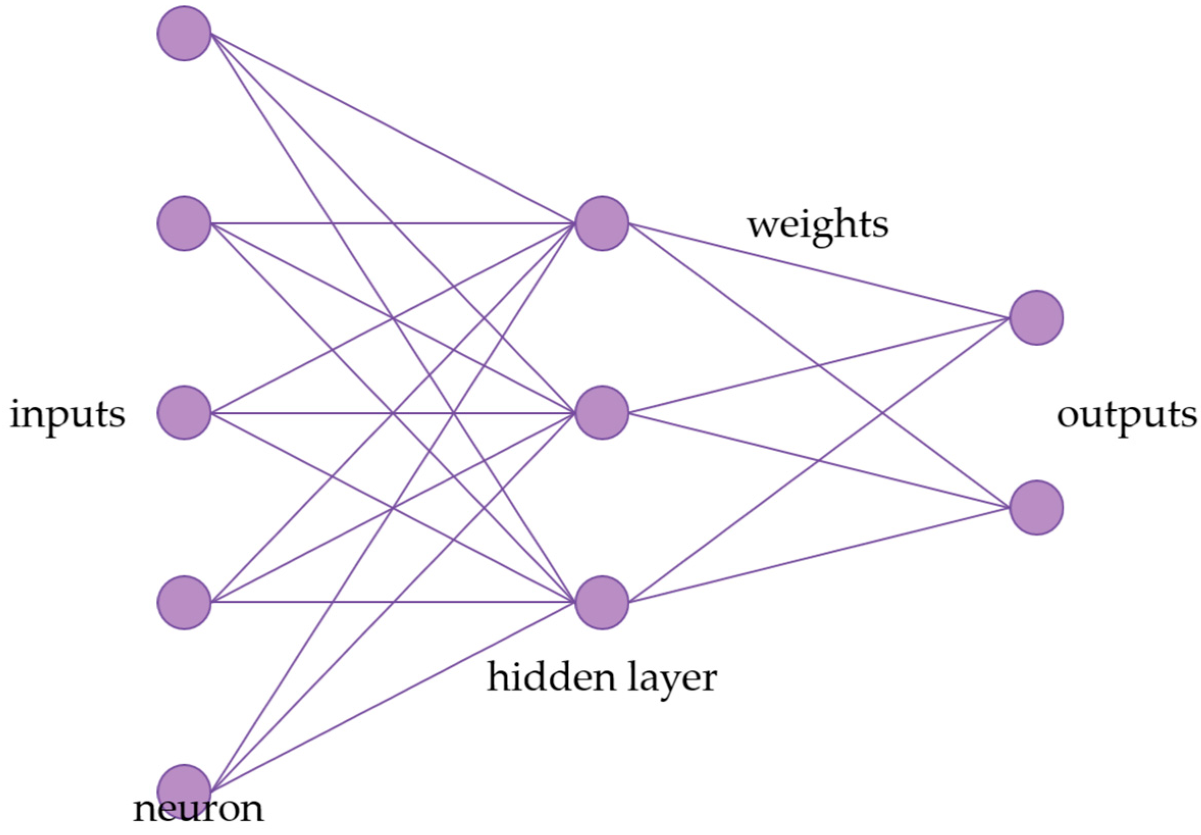
ML models require an appropriate configuration of hyperparameters to ensure optimal performance. Hyperparameters are parameters set prior to the learning process, which influence how the model is trained and how well it generalizes. For instance, in ANNs, defining the number of neurons in the hidden layers is essential according to the specific application. To avoid overfitting during hyperparameter optimization, the dataset was randomly divided into two subsets: a validation set comprising 8000 instances and an evaluation set with 12,000 instances. The validation set was used exclusively for hyperparameter tuning, while the evaluation set was reserved for assessing model performance after optimization.

Hyperparameter tuning uses the Grid Search with Cross-Validation (Grid Search CV) technique. This method exhaustively explores all possible combinations of selected hyperparameters and identifies the set that provides the best performance based on a chosen metric. The performance of the models during hyperparameter optimization was evaluated through the coefficient of determination (R²), defined by Equation (2).

$$R^2=({\displaystyle \frac{\sum \left(e_i-\overline{e}\right)\left(p_i-\overline{p}\right)}{\sqrt{{\sum \left(ei-\overline{e}\right)}^2}.\sqrt{\sum {\left(p_i-\overline{p}\right)}^2}}}{)}^2$$

(2)

where e_i is the carbonation depth value calculated by the deterministic equation, $\overline{e}$ is the mean of the deterministic carbonation depths, p_i is the carbonation depth value predicted by the ML model, and $\overline{e}$ is the mean of the predicted values.

For the RF model, the hyperparameters investigated were min_samples_split, tested with values of 0.01, 0.005, and 0.0025, and max_features, tested with values of 10, 8, 6, and 4. The min_samples_split parameter defines the minimum number of instances required to split a node, while max_features specifies the number of features considered at each split [36]. Additionally, the number of estimators (n_estimators)—representing the number of trees in the forest—was tested with values of [1, 5, 10, 20, 30, 50, 100, 150, 200, 300, 400, and 500], with the best performance achieved using 500 estimators. The optimal configuration for RF was obtained with min_samples_split = 0.0025 and max_features = 10.

For the SVR model, the parameters evaluated included the kernel function, which was fixed as ‘rbf’, the penalty parameter C, with tested values of 1, 1024, 2048, 4096, and 10,000, and the margin of tolerance epsilon, with values of 0.30, 0.25, 0.20, 0.15, 0.10, and 0.05. The kernel function enables the model to handle nonlinear relationships; the penalty parameter C controls the trade-off between achieving a low error on the training data and maintaining a simplified decision boundary; and epsilon defines the width of the margin within which no penalty is applied to errors [36]. The best performance for SVR was achieved with kernel = rbf, C = 10,000, and epsilon = 0.30.

Regarding the ANN, the hyperparameters tested were the initial learning rate (learning_rate_init), evaluated with values of 1, 0.1, 0.01, and 0.001, the number of neurons in the hidden layer (hidden_layer_sizes), tested with configurations of (100), (50), (25), and (10), and the maximum number of training iterations (max_iter), tested with values of 500, 200, 100, 50, 25, and 10. The learning_rate_init controls the magnitude of updates to the model’s weights during training; the hidden_layer_sizes parameter defines the model’s capacity to capture complex patterns; and the max_iter parameter sets the limit for the number of training epochs [53]. The ANN model performed best with learning_rate_init = 0.001, hidden_layer_sizes = (100), and max_iter = 500.

A fixed random state was employed to ensure the reproducibility of the results and facilitate the future replication of the study by other researchers. For the RF model, random_state was set to 10, and for the ANN model, random_state was set to 1. The random_state parameter controls the internal randomization processes of each model, such as the initial split of samples in RF or the initial weights in the ANN, ensuring consistent results across multiple runs. This practice is particularly recommended in ML applications involving stochastic components.

After identifying the best hyperparameter configuration for each model, the evaluation set containing 12,000 instances was used to validate model performance. To ensure a robust assessment, a five-fold cross-validation procedure was adopted. This approach divided the evaluation set into five parts, which were alternately used as the validation set. In contrast, the remaining parts were used for training, thus ensuring that each instance contributed to the training and validation phases.

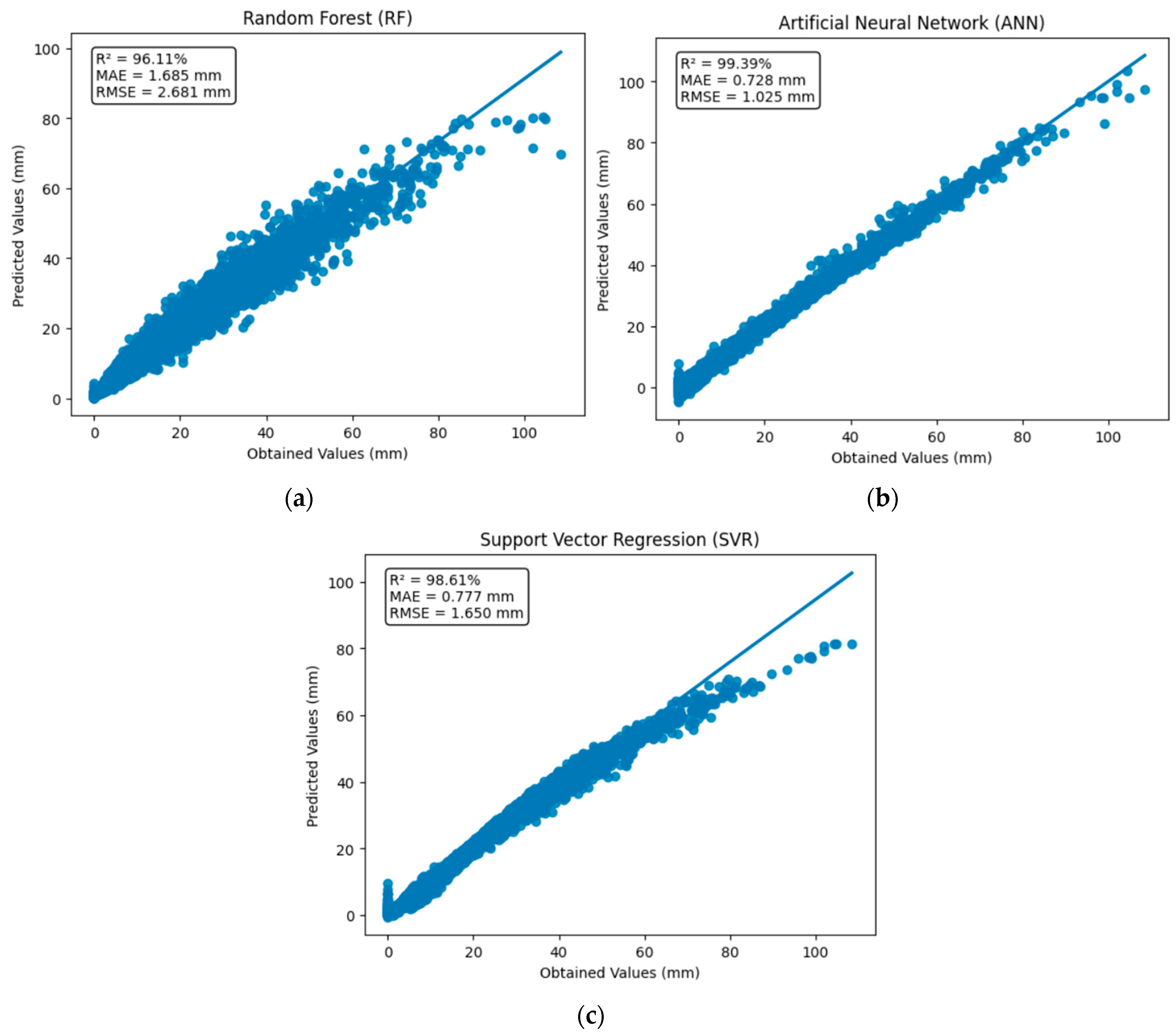
For the final performance evaluation of the models, besides the coefficient of determination (R²), the mean absolute error (MAE) and the root mean square error (RMSE) were also calculated, according to Equations (3) and (4).

$$MAE={\displaystyle \frac{1}{n}}\sum _{i=1}^n|e_i-p_i|$$

(3)

$$RMSE=\sqrt{{\displaystyle \frac{1}{n}}\sum _{i=1}^n{(e_i-p_i)}^2}$$

(4)

where e_i is the carbonation depth value obtained by the deterministic equation, p_i is the carbonation depth predicted by the ML model, and n is the total number of instances.

The evaluation metrics obtained allowed for a complete comparison of the predictive capacity of each ML method in forecasting carbonation depth in RC, thus ensuring the reliability of the adopted models for different scenarios.

2.3. Analysis of Carbonation Feature Behavior Using ML Methods

Different scenarios were created by varying one feature at a time while keeping the others constant to evaluate the behavior of the carbonation features in carbonation depth prediction.

Table 5. Features and adopted values for different analysis scenarios.

Scenario	Varying Feature	Adopted Values	Fixed Features
1	CO2 Concentration (CCO2)	0.03–0.3%	fc = 30 MPa, UR = 60%, Cement = CPII E, Exposure = AEP, Time = 50 years
2	Concrete Strength (fc)	20–50 MPa	CCO2 = 0.1%, UR = 60%, Cement = CPII E, Exposure = AEP, Time = 50 years
3	Relative Humidity (UR)	30–90%	CCO2 = 0.1%, fc = 30 MPa, Cement = CPII E, Exposure = AEP, Time = 50 years
4	Time (t)	0–100 years	CCO2 = 0.1%, fc = 30 MPa, UR = 60%, Cement = CPII E, Exposure = AEP
5	Type of Cement	CPII E, CPII F, CPII Z, CPIII, CPIV, CPV	CCO2 = 0.1%, fc = 30 MPa, UR = 60%, Exposure = AEP, Time = 50 years
6	Exposure Condition	AIP, AEP, AED	CCO2 = 0.1%, fc = 30 MPa, UR = 60%, Cement = CPII E, Time = 50 years

summarizes the features, the adopted fixed values, and the range of variation for each scenario. For each scenario, carbonation depth was predicted as a function of the varying features, and the performance of the ML models (SVR, ANN, and RF) was assessed using the coefficient of determination (R²), mean absolute error (MAE), and root mean square error (RMSE).

Additionally, graphs were generated showing the relationship between carbonation depth and each feature under study, allowing a visual comparison of the models’ behaviors.

For each case, the analysis aimed to understand the sensitivity of carbonation depth predictions concerning each feature, contributing to a better comprehension of feature importance and model performance robustness under different conditions.

3. Results

3.1. Evaluation of the Performance of ML Methods

After generating the synthetic dataset and defining the optimal hyperparameters for each computational model, the performance metrics—R², MAE, and RMSE—were calculated as the averages of the five folds from the CV process to evaluate the predictive capability of each method.

Table 6. Summary of performance metrics for ML methods in predicting carbonation depth.

Method	R2	MAE (mm)	RMSE (mm)
RF	96.11%	1.685	2.681
ANN	99.39%	0.728	1.025
SVR	98.61%	0.777	1.650

summarizes the metric values obtained for the RF, ANN, and SVR models.

The results show that the ANN model achieved the best overall performance, followed by the SVR model. Although the RF model exhibited satisfactory predictive capability, its precision was lower than the other methods. These results demonstrate the effectiveness of ML techniques in accurately estimating carbonation depth in RC structures.

The dispersion plots shown in Figure 4 illustrate the relationship between the observed carbonation depths obtained using the deterministic model and the predicted values from each computational method, along with their respective performance metrics.

As observed in Figure 4, the ANN model stands out for its exceptional ability to fit the data, particularly for higher carbonation depth values, where it maintained high accuracy with minimal dispersion. The SVR model also performed well, presenting slightly greater deviation at higher carbonation depths. This outcome may be attributed to the limited number of instances within this range, affecting the model’s generalization. Despite yielding a reasonable overall fit, the RF model exhibited larger error metrics, reinforcing its lower accuracy compared to the ANN and SVR for this dataset.

Additionally, in the CV process for all three models (SVR, ANN, and RF), the performance metrics for each fold yielded consistent and close results, with no significant deviations observed. This outcome indicates that the models did not overfit the training data. When the metrics are stable across different folds, it suggests that the models are generalizing well and performing consistently rather than fitting too specifically to one particular subset of the data. Overfitting would typically manifest as large variations in performance metrics between folds, where a model performs well on some folds but poorly on others. The consistency observed across folds supports the conclusion that overfitting was not a concern in these models.

Overall, the analysis confirms the high potential of ML methods to model complex, nonlinear processes such as carbonation in concrete structures with high precision. Furthermore, the promising results achieved, particularly by the ANN and SVR, suggest that these techniques could be successfully extended to predict other deterioration phenomena in civil engineering, such as chloride ingress, sulfate attack, or even broader applications in materials science, structural health monitoring, and infrastructure asset management. Through the harnessing of ML, it becomes possible to develop more robust predictive models that assist in optimizing maintenance strategies, improving durability design, and supporting the sustainable management of critical infrastructure systems.

3.2. Analysis of Carbonation Feature Behavior

Six different scenarios were analyzed to investigate the impact of individual features on the carbonation depth prediction, each varying a single feature while maintaining the others at fixed values, as summarized in

Table 7. Summary of performance metrics for ML methods in predicting carbonation depth by scenario and varying feature.

Scenario	Varying Feature	Method	R2 (%)	MAE (mm)	RMSE (mm)
1	CO2 Concentration (CCO2)	RF	87.44	1.710	1.751
		ANN	98.41	0.729	0.732
		SVR	98.41	0.048	0.081
2	Concrete Strength (fc)	RF	99.31	0.952	1.280
		ANN	99.89	0.714	0.772
		SVR	99.90	0.241	0.379
3	Relative Humidity (UR)	RF	94.68	1.690	2.017
		ANN	99.79	0.647	0.748
		SVR	99.97	0.204	0.310
4	Time (t)	RF	98.96	1.317	1.617
		ANN	99.45	0.654	0.840
		SVR	99.88	0.130	0.281
5	Type of Cement	RF	91.84	2.012	2.534
		ANN	99.82	0.686	0.712
		SVR	99.75	0.200	0.270
6	Exposure Condition	RF	99.77	1.038	1.109
		ANN	99.67	0.399	0.458
		SVR	99.99	0.283	0.350

.

In Scenario 1, the CO₂ concentration was varied from 0.03% to 0.3%, with the other parameters held constant. Figure 5 presents the predictions of the SVR, ANN, and RF models obtained under these conditions. It is observed that the SVR model captures an almost linear increase in carbonation depth, closely following the trend predicted by the Possan equation [20], with depth values ranging from approximately 23.2 mm to 24.5 mm. The ANN model also exhibits a positive trend but with slightly higher carbonation depths, between 23.9 mm and 25.2 mm, suggesting a tendency to overestimate the effect of CO₂ concentration. The RF model, by contrast, shows nearly constant predictions between 22.0 mm and 22.2 mm, failing to capture the influence of CO₂ concentration adequately. Although the overall magnitude of error remains low (approximately 2.5 mm at most), it is critical to evaluate how each model tracks the trends induced by variations in the input features. Thus, SVR demonstrates superior sensitivity to continuous variations in the data, while RF shows limitations.

In Scenario 2, the concrete compressive strength (fc) was varied between 20 MPa and 50 MPa. Figure 6 shows the predicted carbonation depths. A clear decreasing trend in carbonation depth is evident as the concrete strength increases, which aligns with the expected physical behavior since higher-strength concretes typically exhibit reduced porosity and permeability [54]. The SVR and ANN models accurately follow the decreasing trend observed in the Possan equation predictions, although the ANN shows minor deviations at higher strengths. The RF model underestimates carbonation depths at lower strengths.

Scenario 3 focused on varying relative humidity from 30% to 90%, with the other parameters fixed. The results in Figure 7 exhibit an inverted parabolic relationship, with carbonation depth peaking at around 50–70% relative humidity, consistent with established behavior [55]. SVR closely matches the Possan equation prediction, accurately tracking the parabolic curve across the entire humidity range. The ANN also captures the general pattern but slightly overestimates carbonation depth near the curve’s peak. RF, however, shows a tendency toward linearization, particularly at higher humidity levels, leading to less accurate predictions.

In Scenario 4, the carbonation depth was predicted as a function of time, varying from 0 to 100 years. Figure 8 illustrates the results obtained for each method. All models correctly captured the increasing trend in carbonation depth over time, but differences emerged in model precision. SVR closely followed the Possan equation across the entire time range, while the ANN also demonstrated good accuracy, with minor discrepancies at longer times. RF, however, progressively underestimated carbonation depth beyond approximately 50 years.

Scenario 5 analyzed the impact of type-of-cement variation, considering CPII E, CPII F, CPII Z, CPIII, CPIV, and CPV-ARI. Figure 9 shows the predictions for each type of cement. The SVR model again demonstrated the closest alignment with the Possan equation across most cement types. The ANN produced consistent predictions but exhibited slight deviations for CPIII and CPIV cements. RF consistently showed larger deviations, especially for CPIV.

Finally, in Scenario 6, the exposure conditions varied among Protected Indoor (AIP), Protected Outdoor (AEP), and Unprotected Outdoor (AED) environments. Figure 10 illustrates the carbonation depth predictions under these conditions. SVR and the ANN agreed with the Possan equation predictions for AIP and AEP exposures, while the ANN performed slightly better for AED exposure conditions. RF exhibited greater deviations across all exposure conditions.

In the sensitivity analysis, the SVR model exhibited higher responsiveness to variations in individual features compared to the ANN and RF models. This behavior is attributed to the inherent characteristics of the algorithms. SVR employs a margin-based optimization approach with kernel functions that accentuate variations near the decision boundary, leading to greater sensitivity to feature changes. In contrast, due to its multi-layer perceptron structure and nonlinear activation functions, the ANN naturally introduces a smoothing effect, reducing its sensitivity to marginal variations in the input features.

It is also noteworthy that the ANN required significantly lower computational resources than SVR, which demanded considerable processing time and memory due to the quadratic complexity associated with kernel methods when applied to large datasets. As a potential improvement, increasing the number of neurons in the hidden layers (hidden_layer_sizes) and the number of iterations (max_iter) could enhance the ANN’s ability to capture more detailed feature interactions. Nevertheless, such adjustments would also lead to higher computational requirements, which must be carefully evaluated depending on the context of the application.

The consolidated performance evaluation metrics for all scenarios are presented in Table 7, allowing a direct comparison of the predictive accuracy of each technique for the different feature variations. The analysis confirms that SVR consistently provided the most accurate and robust predictions, closely matching the expected behavior across the entire range of feature variations. The ANN also demonstrated strong predictive capabilities, while RF exhibited greater variability and occasional underestimations.

These findings emphasize the high potential of advanced ML techniques for modeling complex deterioration mechanisms in materials. Beyond carbonation prediction in concrete, the methodologies developed in this study can be extended to various fields, such as chloride ingress modeling, sulfate attack assessment, freeze–thaw damage prediction, and degradation studies in metallic structures, polymers, and composites. Furthermore, the rigorous application of ML techniques can significantly contribute to infrastructure health monitoring, predictive maintenance, and the sustainable management of assets across different engineering and materials science sectors.

4. Discussion

The feature behavior analysis using the generated dataset reveals relevant findings regarding the performance of the ML models. SVR demonstrated a strong ability to capture linear and nonlinear feature variations, consistently delivering reliable results. This performance can be attributed to the model’s inherent capacity to balance complexity and error tolerance, making SVR particularly effective in scenarios characterized by moderate variability. However, as observed in Figure 4, the SVR model exhibited lower accuracy for extreme carbonation depths (e > 80 mm), likely due to the reduced data density in this range.

Nonetheless, technical standards [52,56] specify minimum concrete cover requirements typically between 20 mm and 50 mm, depending on environmental aggressiveness. Therefore, the margin of error observed for depths beyond these normative limits is less critical for practical applications. SVR’s predictive performance within these typical intervals is sufficiently robust to ensure durability assessments and structural protection under real exposure conditions.

The ANN model attained the highest R² among all evaluated techniques, demonstrating excellent performance, particularly for higher carbonation depths where its predictions closely matched the expected trends. However, its more complex network structure makes it somewhat more susceptible to overfitting, especially in regions with limited data representativity. It is also important to note that deeper neural networks (DNNs) or convolutional neural networks (CNNs) were not considered in this study, as the dataset is tabular and of moderate size. The selected ANN configuration already delivered very satisfactory results, and further improvements could potentially be achieved through more refined hyperparameter optimization rather than by increasing model complexity.

While achieving reasonable results in terms of overall metrics, the RF model demonstrated limitations in accurately capturing subtle feature variations. RF’s ensemble structure, although robust against overfitting, tended to oversimplify nonlinear relationships, as seen in the CO₂ concentration and relative humidity scenarios. Improvements could involve hybridization with other algorithms or more aggressive hyperparameter tuning.

Regarding the comparative behavior of the models, it is important to emphasize that SVR demonstrated higher feature sensitivity in the sensitivity analysis, which can be attributed to its margin-based optimization and kernel functions. However, this higher sensitivity came at the expense of greater computational demands when compared to the ANN, which, despite showing a smoother response to feature variations, required significantly fewer computational resources. This trade-off highlights the need for careful hyperparameter tuning and model selection according to the specific application context, balancing accuracy, interpretability, and computational efficiency.

A critical aspect to highlight is that the major contribution of this research is not confined to carbonation modeling itself but rather lies in the methodological advancement of ML applications for complex durability phenomena. The techniques employed—RF, SVR, and ANNs—are generic and highly adaptable, thus positioning this study as a methodological contribution that can be transferred to any degradation mechanism or material system where multi-factor interactions govern performance over time.

Equally important is the strategic use of synthetic datasets, especially in fields where obtaining comprehensive real-world data is unfeasible within reasonable timeframes. In the case of carbonation, natural exposure tests can take years or even decades to produce measurable results [57]. By using a validated mathematical model (Possan equation [20]) to generate a large and controlled dataset, this study enables the rapid, systematic evaluation of ML models while faithfully preserving the core relationships between key variables. Thus, synthetic data generation emerges as a powerful research tool that not only accelerates the development of predictive models but also ensures a broader and more diversified feature space than traditional experimental studies.

Moreover, it is important to emphasize that the use of synthetic datasets for carbonation prediction remains largely underexplored in the existing literature. As identified in recent reviews, the vast majority of ML models for carbonation have been trained on small experimental datasets, often mixing results from accelerated and natural tests, which can introduce inconsistencies and biases [31,58]. Only a few studies, such as Martínez-Muñoz et al. [21], have demonstrated the high potential of synthetic datasets in structural engineering by generating large and systematically varied datasets, achieving high model accuracy and enabling multi-objective optimization. In the field of carbonation, where natural exposure data are extremely slow to obtain, synthetic datasets offer a particularly promising pathway to overcome the scale, speed, and variability limitations that traditionally hinder the development of robust predictive models. By adopting a synthetic approach, this study aligns with the emerging perspective that when properly validated, synthetic datasets can significantly accelerate innovation and reliability in durability modeling.

Notably, the ML models developed in this study are trained exclusively on data generated from the Possan equation, which, although widely used and validated in the literature, presents inherent simplifications. The equation assumes constant CO₂ concentrations and homogeneous materials and does not fully capture complex interactions such as time-dependent diffusivity, carbonation-induced porosity changes, or multi-phase transport phenomena. Consequently, these limitations are inevitably propagated into the ML models, restricting their capability to represent some real-world carbonation scenarios, particularly under variable environmental exposures or unconventional material compositions. Future research should explore the integration of hybrid datasets combining experimental data, probabilistic models, or multiphysics simulations to overcome these limitations and enhance the robustness and generalization of ML applications in carbonation modeling.

Beyond structural engineering, the methodologies and strategies developed here are highly transferable. ML models optimized through synthetic datasets can be applied to predict deterioration phenomena such as chloride ingress, sulfate attack, freeze–thaw cycles, alkali–silica reaction, and even degradation in polymeric, metallic, and composite materials. Therefore, this study positions itself as a methodological benchmark for the broader integration of ML into durability modeling and infrastructure resilience planning.

5. Conclusions

This paper applied ML models (RF, SVR, and ANN) to predict carbonation depth in RC structures using a large synthetic dataset derived from the Possan equation. Beyond the specific application to carbonation, the research emphasizes the methodological advances associated with ML techniques and the strategic use of synthetic data in scenarios where experimental data are scarce or time-consuming to collect. The following conclusions can be drawn:

• The comparative analysis of model performance demonstrated that the ANN achieved the highest predictive accuracy, followed closely by SVR, while RF exhibited lower precision, particularly for features with nonlinear behavior. SVR proved especially robust in capturing linear and nonlinear trends, making it a reliable choice for scenarios with moderate feature variability. Despite its slightly higher susceptibility to overfitting, the ANN consistently provided accurate predictions even at higher carbonation depths.
• The behavior analysis of individual features highlighted the influence of compressive strength, exposure time, and relative humidity as the primary factors affecting carbonation depth. Increasing compressive strength reduced carbonation due to lower porosity, while longer exposure times naturally promoted carbonation progression. Relative humidity exhibited an inverted parabolic effect, with maximum carbonation around 50–70%, which aligns with established physical principles. Cement type and exposure conditions also impacted results, while CO₂ concentration played a comparatively smaller role under simulated conditions.
• This study confirms that ML models can replicate complex physical behaviors embedded in deterministic models, validating their use for carbonation and broader durability assessments. The models successfully tracked known dependencies, such as the reduction in carbonation with higher concrete strength and the nonlinear relationship with relative humidity, indicating their potential for data-driven durability predictions.

It is worth mentioning that despite the promising results, some limitations must be acknowledged. Using a synthetic dataset, while allowing controlled and diversified scenario analysis, inherently reflects the assumptions and constraints of the mathematical model (Possan equation) on which it is based. Furthermore, the absence of validation against real-world experimental data restricts direct extrapolation to practical applications without caution. The lower density of instances for extreme carbonation depths (>80 mm) affected model accuracy in these regions, although these conditions exceed typical service life criteria defined by technical standards [52,56].

At this stage, no experimental datasets were incorporated for model benchmarking. As a future development, the incorporation of small-scale experimental datasets is recommended to benchmark and verify the robustness of the trained models, particularly for carbonation depths within the typical service life range. The availability of an open access dataset for benchmarking purposes is also noteworthy, at https://carbuai.pythonanywhere.com/ (accessed on 27 April 2025).

Overall, this study reinforces the value of synthetic datasets for accelerating ML model development in areas where experimental data collection is lengthy and costly, such as carbonation under natural exposure. By demonstrating high predictive accuracy and the ability to capture complex feature interactions, the methodologies developed here offer significant contributions to concrete carbonation studies and the broader field of material degradation modeling. Future research should prioritize hybrid datasets combining synthetic and experimental data, explore hybrid model architectures, and apply the proposed methodologies to other deterioration phenomena, such as chloride ingress, sulfate attack, and freeze–thaw damage. These steps will further expand ML approaches’ practical impact and generalization capability in durability engineering.