Article

Thermodynamic, Economic, and Environmental Multi-Criteria Optimization of a Multi-Stage Rankine System for LNG Cold Energy Utilization

Tianjin Key Laboratory of Clean Energy and Pollution Control, School of Energy and Environment Engineering, Hebei University of Technology, Tianjin 300401, China
*
Authors to whom correspondence should be addressed.
Modelling 2025, 6(2), 45; https://doi.org/10.3390/modelling6020045
Submission received: 4 April 2025 / Revised: 2 June 2025 / Accepted: 5 June 2025 / Published: 9 June 2025

Abstract

Utilizing the considerable cold energy in liquefied natural gas (LNG) through the organic Rankine cycle is a highly important initiative. A multi-stage Rankine-based power generation system using LNG cold energy for waste heat utilization was proposed in this study. Moreover, a comprehensive assessment method was used to select the working fluid for this proposed system. Not only were thermodynamic and economic indicators considered, but also the environmental impact of candidate working fluids was taken into account in the evaluation process. The optimal operating points of the system were determined using non-dominated sorting genetic algorithm II and TOPSIS methods, while employing Gray Relational Analysis was applied to compute the gray relational coefficients of candidate working fluids at the optimal operating points. In addition, four weighting methods were used to calculate the final gray correlation degree of the candidate working fluids by considering the weighting influence. The stability of the calculated gray correlation degree was observed by performing a standard deviation analysis. The results indicate that R245ca was chosen as the optimal working fluid due to its superior performance based on the entropy weighting method, the independent weighting coefficient method, and the mean weighting method. Simultaneously, R245ca exhibits the best specific net power output and levelized cost of energy values of 0.283 USD/kWh and 106.9 kWh/t, respectively, among all candidate working fluids. The gray correlation degree of R1233zd(E) is 0.948, exceeding that of R245ca under the coefficient of variation method. The gray correlation degree under the mean value method is the most stable, with a standard deviation of only 0.162, while the gray correlation degree under the coefficient of variation method exhibits the greatest fluctuation, with a standard deviation of 0.17, in the stability assessment.

1. Introduction

Nowadays, environmental pollution has become increasingly severe, and the development of clean energy is an important way to alleviate environmental pollution. Natural gas is widely used in clean energy due to its good economy and reliable safety [1]. Liquefied natural gas (LNG) is mainly used for long-distance natural gas transportation. Natural gas is compressed and cooled to become LNG for loading and transportation [2]. During transportation, it is necessary to pressurize and liquefy natural gas at low temperatures to reduce its volume and store more natural gas. In the process of use, it needs to be re-gasified and transported to the user end [3]. In the re-gasification process, a heat source is required to exchange heat with natural gas to turn it from a liquid to a gas state. However, most of the re-gasification processes use seawater as a heat source for heat exchange, which not only results in a large amount of waste of thermal energy but also has a certain impact on the ocean [4].
Some technologies that use the cold energy of LNG have been proposed, including low-temperature power generation, seawater desalination, cold energy storage, and food processing [5]. Among them, the organic Rankine cycle (ORC) has received extensive attention due to its safety, reliability, high efficiency, energy saving, and environmental friendliness, becoming an energy utilization technology with broad application prospects and high technical advantages [6]. The ORC is a more promising LNG re-gasification cold energy utilization technology than others [7]. Several methods have been proposed by scholars for LNG cold energy utilization in power generation. Ma et al. [8] used parallel and series configurations of the ORC, Brayton Cycle, and Supercritical Carbon Dioxide Power Cycle to utilize the cold energy of LNG. The results showed that the best combination cycle was a two-stage continuous ORC, with the highest net power output ratio of 202.15 kJ/kg and the lowest leveling cost of electricity at 0.11 USD/kWh. Joy et al. [9] compared the performance of a multi-stage, cascaded ORC using seawater as the heat source and LNG as the cold source. They found that only the two-stage system cascaded with the first stage could reduce the electricity generation by 8.6% compared with the three-stage system. However, the simplicity of the two-stage system cascaded with the first stage greatly improved, and the surface area of the heat exchanger correspondingly decreased by 20%. Huang et al. [10] designed a novel cold–electricity cogeneration system based on refrigeration warehouses, which used the waste heat generated by natural gas power plants as a heat source and LNG as a cold source. They investigated the changes in design performance at different re-gasification rates. The main results showed that compared with traditional systems, the peak-to-valley ratio of the cold–electricity cogeneration system can be significantly increased from 0.4 to 1. The investment payback period of the system can be reduced by half, to 0.67 years.
The working fluid is crucial and directly impacts the performance of the ORC system. Yang et al. [11] utilized a multi-objective genetic algorithm to optimize three combined heat and power systems based on organic Rankine cycles, the outcomes of which can offer guidance for the selection of working fluids. Mohan et al. [12] screened 11 candidate working fluid mixtures based on the output power and thermodynamic efficiency. They found that R600a was the optimal working fluid when taking the maximum output power into account. Hu et al. [
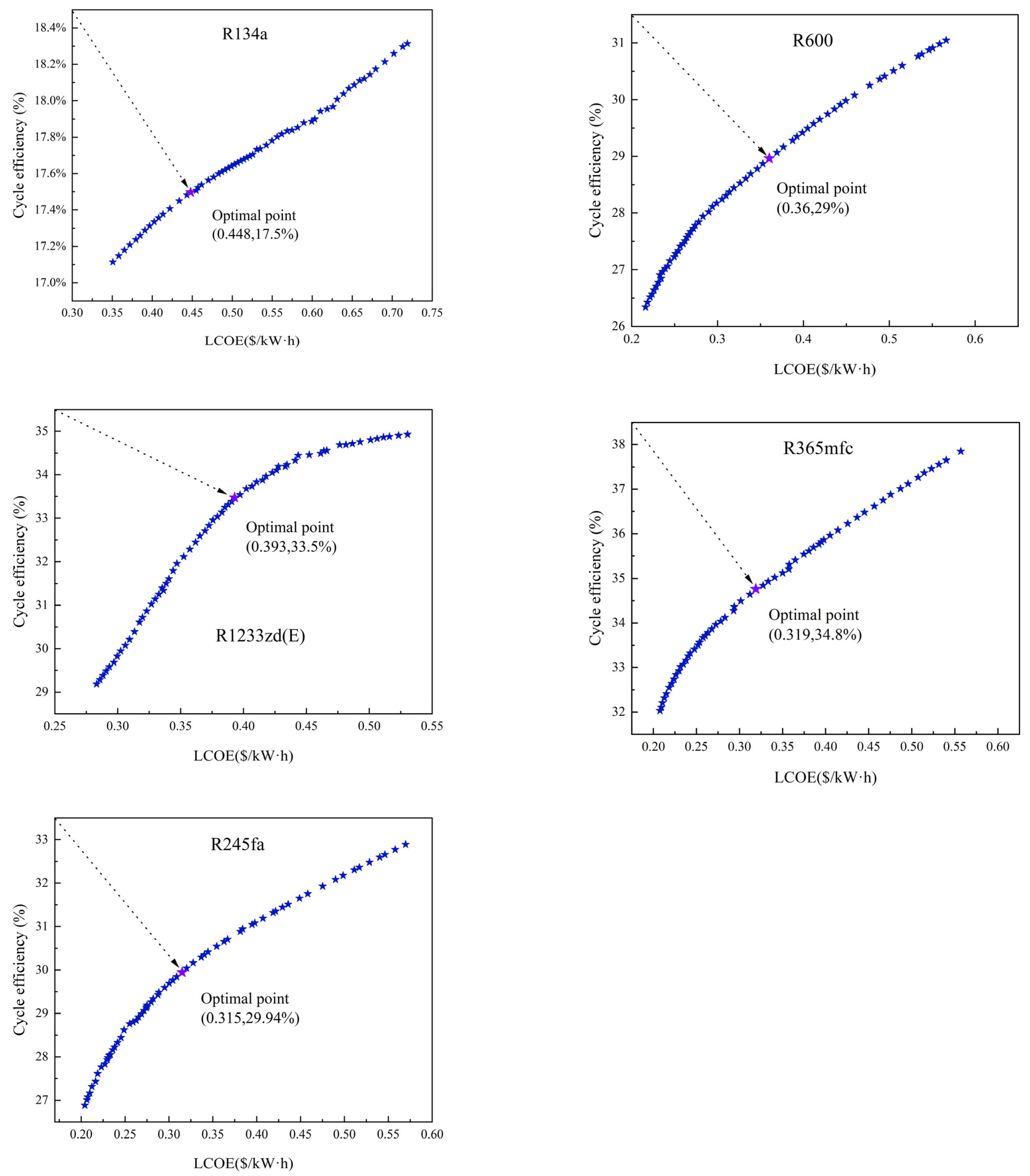
13] established mathematical and physical models for the thermal process of the ORC system. They optimized the process using 245 organic working fluids with unit mass net electricity generation from hot water as the optimization objective. R245fa was selected as the optimal working fluid. In the research focusing on the selection of working fluids, it is imperative not only to consider the thermodynamic and economic performance of the system, but also to engage in a critical discussion regarding the environmental implications.
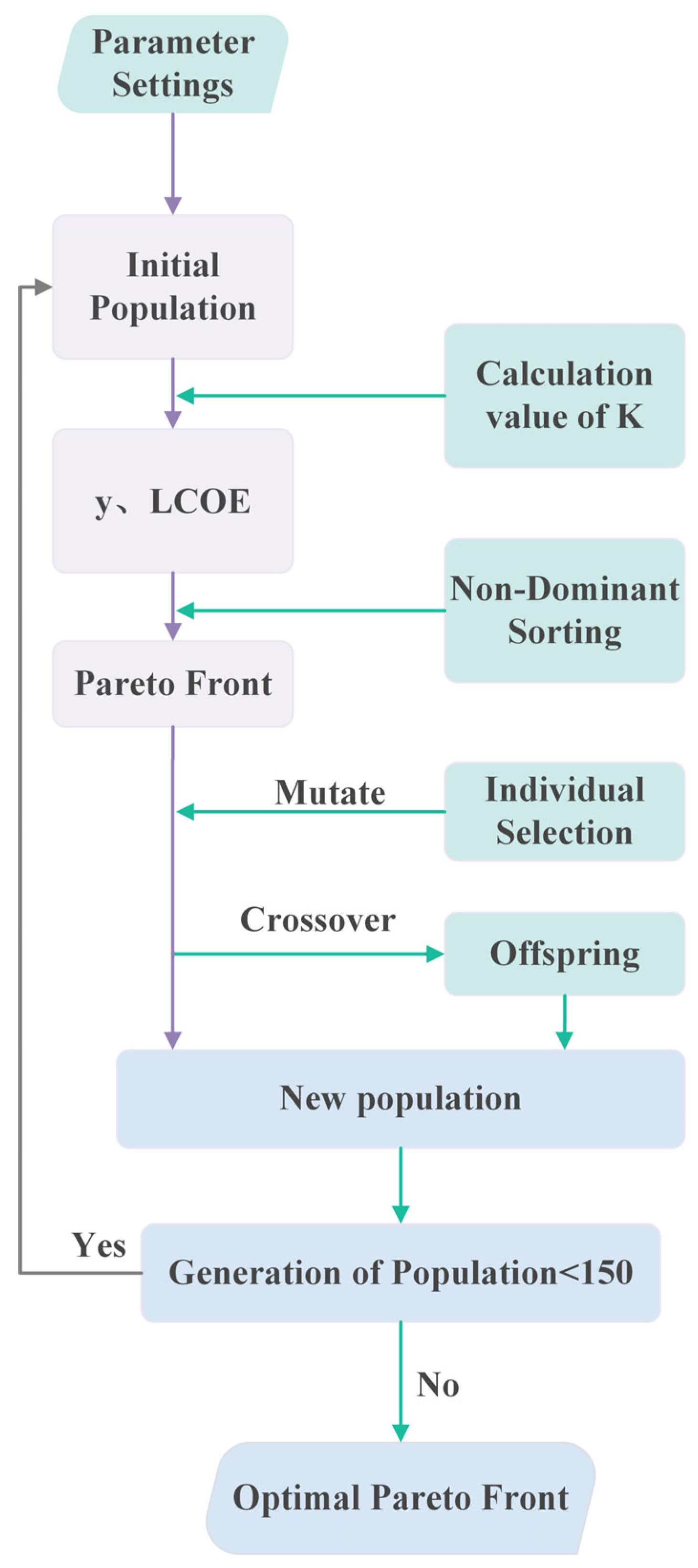
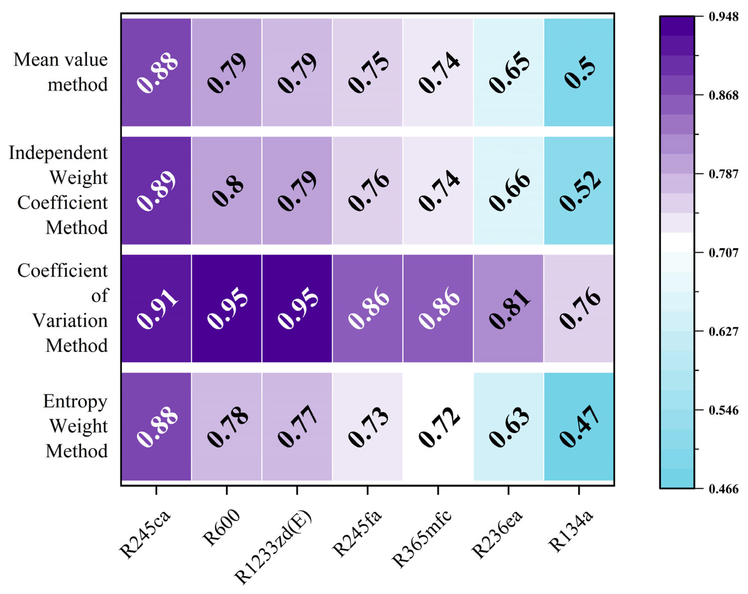
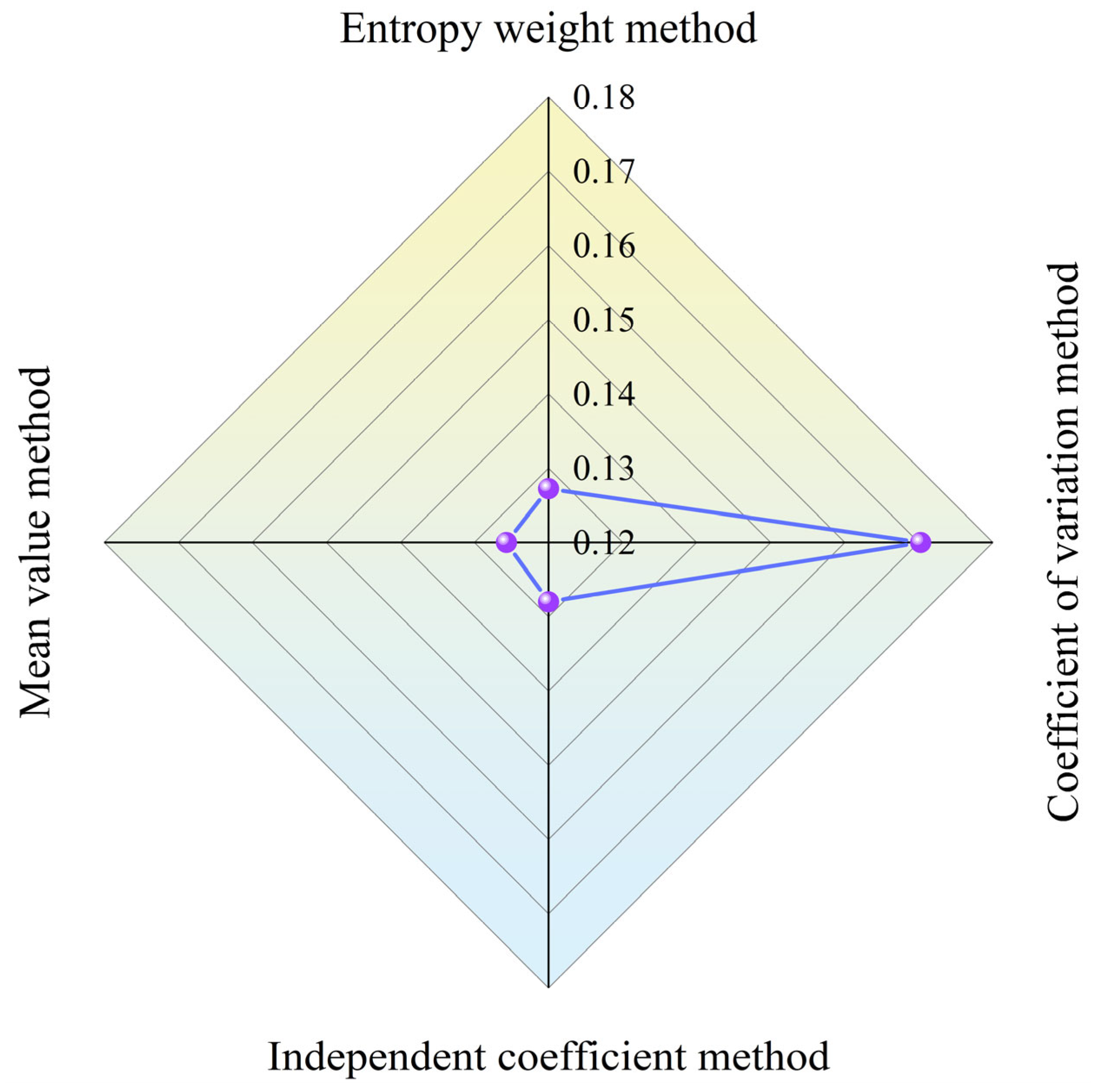
The comprehensive evaluation and optimization decision-making for thermal systems necessitate the consideration of multiple assessment criteria, which are interrelated with the ultimate optimal outcome. The Gray Relational Analysis (GRA) method is based on the gray system theory and can analyze the correlation between each indicator, obtain the influence weightings of each indicator on the comprehensive evaluation results, and make optimization decisions. Mausam et al. [14] used GRA to verify the optimized experimental results of a flat-plate-collector solar energy collection system. They evaluated the performance using the flow rate, intensity, and tilt angle as targets. It was found that the maximum instantaneous efficiency was 2.25% at the flow rate of 68.7 lpm, intensity of 1 W/m2, and tilt angle of 400°. Bademlioglu et al. [15] studied the cycle characteristics of the ORC system and used GRA to optimize and evaluate the main process parameters, including evaporator temperature, turbine efficiency, heat exchanger efficiency, and condenser temperature, to determine the system operating conditions. The findings indicate the first and second law efficiencies of the system were 18.1% and 65.52%, respectively. Wu et al. [16] studied the performance of the ORC system under different load powers based on a built low-temperature waste heat power generation test platform. The analysis showed that there the closest correlation was between the power and load power, with a gray correlation degree of 0.632. In the GRA evaluation, the weighting of each indicator directly affects the accuracy and credibility of the comprehensive evaluation results, with a higher weighting indicating a greater contribution to the comprehensive evaluation results. In the GRA, the assignment of weightings has a direct effect on the final optimization results; however, to date, no publications have isolated the impact of disparate weighting methodologies on the GRA outcomes.
Previous research has shown that cascading or multi-stage ORCs can improve heat-source matching, yet most published schemes still operate with a single evaporator, rely on fixed fluid selections, and neglect the synergistic use of waste heat and LNG cold energy. Moreover, the studies that apply Gray Relational Analysis (GRA) to working fluid screening seldom examine how alternative weighting strategies influence the final decision, leaving important sources of evaluation bias unaddressed.
Against this backdrop, the present work introduces a multi-stage Rankine system driven by waste heat and LNG cold energy (MSR-LNG). The system couples a dual-stage ORC with an LNG expansion module and embeds an internal preheater/recuperator to recover sensible heat between the stages. A comprehensive optimization framework links thermodynamic, economic, and environmental objectives through non-dominated sorting genetic algorithm II (NSGA-II) and TOPSIS, while four distinct GRA weighting schemes are compared to clarify their impact on fluid ranking. By integrating these elements, this study advances the state of the art in three ways: (1) realizes a tighter temperature-glide match between the heat source and sink through a dual-stage topology, reducing irreversibility across the entire temperature span; (2) embeds internal heat recovery, lowering external heat exchange area demand and simplifying pipework; (3) delivers a unified thermo-economic–environmental optimization routine that shows how the weighting method affects fluid selection, providing a transparent basis for material choice; and (4) presents a comparison table later in the paper, which benchmarks these contributions against the representative LNG–ORC studies published in recent years, evidencing the superior conversion performance and lower levelized cost achieved by the proposed configuration.

2. System Description

The flow diagram of the MHUS-MSR-LNG is illustrated in Figure 1. Figure 2 shows the overall process flow diagram for the MSR-LNG cycle.
The MSR-LNG proposed in this article consists of two modules, an ORC module and an LNG module, which are connected by pipes for heat exchange. The red piping represents the waste heat, the purple piping denotes the working fluid circuit, and the blue piping symbolizes the natural gas sub-process.
In Figure 2, the blue line indicates the natural gas treatment process, the pink line is the ground source hot water treatment process, and the purple line indicates the working fluid change process.
The ORC module in the MSR-LNG operates as follows: Exogenous high-temperature waste heat H1 undergoes a dual heat exchange within evaporators 1 and 2 of the waste heat circuit, transforming into low-temperature waste heat H3. Throughout this process, the thermal energy generated from the waste heat can be thoroughly exploited. The liquid working medium F1 absorbs heat within evaporator 1, transmuting into a high-temperature superheated gas F2, which propels the rotation of the expander, consequently driving the coaxial generator to produce electricity. Post-expansion, it becomes a low-temperature gaseous working medium, F3. F3 conveys heat to the liquid working medium F6 within the condenser through the preheater. Subsequently, the temperature of the gaseous working medium F4 decreases. F4 absorbs the cold energy of natural gas and becomes a saturated liquid, F5, in the condenser. After being pressurized by the pump, F5 becomes saturated liquid working fluid F7 after absorbing heat from F6. In this module, the preheater is located after the pumps and heats the spent gas after it passes through the expander by means of the work mass from the condenser. Its main function is to recover the waste heat from the work mass and increase the efficiency.
In the LNG module, LNG L1 needs to be maintained at a suitable temperature and pressure (0.1 MPa, −162 °C) during storage and transportation. It is pressurized by water pump 3 to become L2, which absorbs heat in the condenser and becomes a saturated liquid (L3). L3 exchanges heat with waste heat H2 and becomes a high-temperature gas working fluid (L4), which then cools and depressurizes through expander 2 to become gaseous natural gas that can be directly used.
LNG is considered a multi-component mixture with the molar composition CH4 90.1%, C2H6 5.8%, C3H8 3.0%, n-C4H10 0.6%, i-C4H10 0.3%, N2 0.2%. Thermophysical properties were evaluated with REFPROP 10.0, which accounts for the non-ideal phase behavior of cryogenic mixtures.
By splitting the evaporation process into two temperature-matched stages, the dual-stage Rankine configuration markedly narrows the average temperature difference between each evaporator and its heat source, which in turn suppresses irreversibilities on the heat-addition side. Combined with an internal recuperator, the layout yields a clear improvement in the overall second-law efficiency. Compared with a conventional single-stage ORC, this architecture achieves a pronounced enhancement in thermoelectric conversion performance, yet it preserves the compactness and modularity that make ORC systems attractive, since both stages share a single generator shaft and control loop and therefore require no extra major equipment.
The paper is aimed at (i) academic researchers working on thermodynamic cycle modeling and (ii) process engineers of LNG re-gasification and low-temperature waste-heat recovery.

3. Methods

3.1. Thermodynamic Model

Geothermal energy is a clean energy source, so the waste heat is the price MSR-LNG pays when it outputs electricity, and the thermal–electric efficiency is selected as an evaluation index for the system’s cycle efficiency [17]:
η = W n e t Q e v a p 1 + Q e v a p 2
where W n e t represents the net power output of the MSR-LNG. Q e v a p 1 is the heat transfer rate in evaporator 1, while Q e v a p 2 denotes the heat transfer rate in evaporator 2. Table 1 shows the energy equation for each component in detail.
The formula to calculate W n e t is as follows:
W n e t = W exp e 1 + W exp e 2 W p u m p 1 W p u m p 2 W p u m p 3 W p u m p 4
where W exp e 1 is the electricity generation from the ORC module expender 1, W exp e 2 represents the electricity generation from the LNG module expender 2. h characterizes the enthalpy of the working fluid state point and m f represents the mass flow rate of the working fluid.
The specific net power output (SNPO) is a key performance metric in the context of natural gas power generation. It typically refers to the net power output per unit mass flow rate of the natural gas fuel consumed. It can be defined using Equation (6), and its unit is kWh/t.
S N P O = W exp e 2 W p u m p 3 m l
where m l denotes the mass flow rate of natural gas.

3.2. Economic Model

The economic performance can be used to assess the feasibility of this proposed system. It is a crucial indicator for the application of the proposed MSR-LNG. The levelized cost of energy (LCOE) is a commonly used metric for evaluating the economic viability of different power generation technologies [19]. It represents the cost of electricity generation over the entire lifespan of a power plant. In this paper, the LCOE is used to assess the feasibility of the MSR-LNG, and it can be calculated as follows:
L C O E = C a n + i = 1 n A c ( 1 + r ) i i = 1 n W n e t ( 1 + r ) i
where A c is the annual operational cost, A c is 1.5% of C a n , and i characterizes the life of the system. It is set to 20 years in this paper; W n e t is the annual total electricity generation. r is the discount rate; 5% is the real (inflation-free) discount rate (the analysis reflects OECD financing conditions and provides sensitivity guidance for 8–10% rates). C a n is the total initial investment cost [20] and can be calculated as the following Equation (8):
C a n = C P M + C w 1 C 2019
C 2019 = C ref × CEPCI 2019 CEPCI ref
where C P M represent the initial investment cost for the evaporator, condenser, preheater, expander, and pump. C w is the initial investment cost for the heat source. C ref is the cost in the original reference year. C 2019 is 607.5.
C P M can be calculated by the following equations:
C P = C P F B M = C P ( B 1 + B 2 F M F P )
log C P = K 1 + K 2 log x + K 3 ( log x ) 2
log F P = C 1 + C 2 log P + C 3 ( log P ) 2
The cost of the component is represented by C P ; the material correction factor and pressure correction factor are denoted as F B M and F P , respectively. The heat exchanger area or power generation is indicated by x . Table 2 displays the values of the correction factors mentioned.
The cost correlations adopted are based on CEPCI basis 2019. All component capacities obtained in this study fall within the limits presented; thus, no extrapolation of the functions was required.
The total heat exchange area of the heat exchangers can be calculated by the following equations:
A = Q K F Δ T l m
where F is the correction factor of the logarithmic mean temperature difference, which has a value of 1. Δ T l m is the logarithmic average temperature of the heat exchangers. K is the total heat transfer coefficient.
Δ T l m can be calculated as:
Δ T l m = ( T h , 1 T f , 2 ) ( T h , 2 T f , 1 ) l n ( T h , 1 T f , 2 ) ( T h , 2 T f , 1 )
K denotes the total heat transfer coefficient, which is:
K = 1 h b d 0 d i + d o 2 λ ln d o d i + 1 h g
The present study employs a shell-and-tube heat exchanger, where h g and h b refer to the convective heat transfer coefficients of the tube and shell sides, respectively. d i and d 0 denote the inner diameters of the tube and shell sides, respectively. λ represents the heat transfer coefficient of the fluid inside the tube. Due to the difference in heat transfer processes, calculations need to be performed separately for the evaporator and condenser, while the k value of the preheater can be calculated using the evaporator section.
(1)
Evaporator
To enhance heat transfer, the hot source flows on the shell side while the working fluid flows on the tube side. For the single-phase flow of the hot source in the evaporator shell side, the Nusselt number is calculated using the Dittus–Boelter equation:
N u = 0.023 R e 0.8 P r n
where R e is the Reynolds number and P r is the Prandtl number. The evaporator is heated and cooled, n, take 0.4 and 0.3, respectively. The heat exchanger tube has three regions: liquid, two phase, and gas. The calculation formula for the working fluid in the liquid region is as follows [22]:
N u = ( f / 8 ) ( R e 1000 ) P r 1 + 12.7 ( f / 8 ) 0.5 ( P r 2 / 3 1 )
f denotes the friction factor:
f = 0 . 79 ln Re 1 . 64 2
The heat transfer coefficient when the working fluid is in the gas–liquid two-phase region is [23]:
α TP = α LS F
α LS = 0.023 G ( 1 x ) D μ 1 0.8 P r L 0.4 k 1 D
F = 1.0 , 1 X t t 0.1
F = 2.35 1 X t t + 0.213 0.736 , 1 X t t > 0.1
X t t = 1 χ χ 0.9 ρ g ρ I 0.5 μ 1 μ g 0.1
The following equation is used when the working fluid is in the gaseous state:
N u = 0.71 R e 0.5 P r 0.36 P r P r W n
P r W is the Prandtl number of the fluid at the temperature of the smooth outer wall.
(2)
Condenser
The working fluid flows in the shell side, and the shell side of the heat exchanger is divided into two zones during the heat transfer process: the gas zone and the gas–liquid two-phase zone. The working fluid is cooled in the gas zone, and the Nusselt number can be calculated using Equation (23) to determine the rate of heat transfer. When the working fluid is in the gas–liquid two-phase zone, the Nu for the heat transfer process is given by [24]:
N u = 0.729 g ρ f ρ f ρ g d o 3 h fg μ k λ r ( T sat T wall ) 0.25
On the tube side, liquefied natural gas (LNG) flows from a subcooled liquid state to a saturated liquid state, and the flow is characterized by a single-phase turbulent flow. The Nusselt number can be calculated using Equation (15).

3.3. Multi-Objective NSGA-II Optimization Algorithm

NSGA-II is an advanced and enhanced multi-objective optimization algorithm that employs non-dominated sorting, crowding distance, and genetic mutation techniques to effectively address complex optimization problems with multiple objectives [25].
In this study, NSGA-II was utilized to optimize the conflicting η and LCOE of MSR-LNGs and to identify their Pareto front. The initial population size was set to 100, and after 150 generations, the model achieved convergence. Encompassing evaporating pressure ( P e ), condensing temperature ( T c ), heat source flow rate ( x ), preheater liquid working fluid temperature rise ( Δ T ), and LNG pump pressure ( P L N G ), Figure 3 presents the pseudo-code of NSGA-II, which outlines its optimization process.
The optimization procedure entails specifying a range of variables. The reasons for the choices and the impact on the results are explained in Table 3, each with prescribed limits detailed in Table 4.
P c r , f and P c r , l represent the critical pressure of the working fluid and natural gas, respectively.

3.4. Gray Relational Analysis

Gray Relational Analysis is a multi-factor evaluation method based on the gray system theory, which can be used to study the correlation and contribution among multiple factors. For each factor sequence, GRA calculates its similarity with other factor sequences to obtain the correlation degree of each factor sequence [26]. The higher the correlation degree, the greater the impact of the factor sequence on the research object. The calculation process is as follows:
(1)
Normalize the original sequences (i = 1, 2, 3, …, n; k = 1, 2, 3, … m).
x i k = x i k x i 1 ( i = 1 ,   2 ,   3 ,   ,   n ;   k = 1 ,   2 ,   3 ,   ,   m )
(2)
Select reference sequence x 0 k (k = 1, 2, 3, …, m).
(3)
Calculate correlation coefficients:
ζ i ( k ) = min i min k x 0 ( k ) x i ( k ) + ρ max i max k x 0 ( k ) x i ( k ) x 0 ( k ) x i ( k ) + ρ max i max k x 0 ( k ) x i ( k )
ρ was set to 0.5 in this paper for discrimination purposes.
(4)
Calculate the final correlation degree:
r i = 1 m k = 1 m ω i ζ i ( k )
where ω i represents the weighting of each element.
Weighting is the core parameter that affects the reliability and objectivity of the gray correlation evaluation. In order to avoid result bias created by a single assignment and to verify the robustness of the evaluation system, this paper also adopts the information entropy weighting method, the coefficient of variation method, the independent coefficient method, and the average assignment method, and the specific selection basis and the typical application scenarios are described as follows in Table 5.

3.5. Optimal Operating Point Selection

The iterative analysis of the objective function η and LCOE using NSGA-II was conducted to obtain its Pareto front in Section 3.3. The optimal point is when the objective function η is maximized and the LCOE is minimized, but these two objectives are in conflict and cannot be achieved simultaneously. This requires balancing the two objectives to achieve an overall optimal solution. TOPSIS (Technique for Order of Preference by Similarity to Ideal Solution) is a method used for multi-criteria decision analysis. This method compares decision alternatives with ideal and negative ideal solutions to determine their relative proximity, and thus derive the best decision solution.
TOPSIS first requires standardizing each element of the Pareto front:
L C O E i n = L C O S i L C O S i m i n L C O S i m a x L C O S i m i n
η i n = η i η i m i n η i m a x η i m i n
The closeness factor C l i represents the close distance between a point on the Pareto front and an optimal point. C l i is defined as follows:
C l i = S i S i + S i +
where S i + and S i represent the actual distances between points on the Pareto frontier and the ideal or non-ideal points. They can be calculated as:
S i + = ( L C O E i n L C O E i m i n ) 2 + ( η i n η i m a x ) 2
S i = ( L C O E i n L C O E i m a x ) 2 + ( η i n η i m i n ) 2

3.6. Boundary Conditions

The model assumes the following boundary conditions:
The simulation requires the use of idealized conditions that need to ignore factors such as frictional heat transfer. The boundary conditions need to be simplified and the model assumes the following boundary conditions:
  • Negligible pressure drop in inter-connecting piping.
  • Adiabatic system boundaries.
  • Expander isentropic efficiency is constant (0.85) [17].
  • Uniform working fluid composition.
  • Negligible kinetic and potential energy changes.
  • Perfect heat exchangers outside the pinch constraint.
  • Saturated liquid at pump inlet.
  • Steady-state operation.
  • Enthalpy is constant during valve throttling.

4. Candidate Working Fluids

The working fluid selection markedly influences the system’s efficiency. The apt choice of a working fluid necessitates a consideration of its thermodynamic properties aligning with the system’s operational temperature range and the properties of the heat source. The temperature of the heat source should be higher compared to the boiling point of the working fluid to facilitate effective vaporization at comparatively modest temperatures in the ORC system. During the transition of LNG from a liquid to a gaseous state, there is a need to release substantial refrigeration at low temperatures. The selected working fluid should be capable of efficiently absorbing this refrigeration under the cryogenic conditions of LNG vaporization, meaning that the fluid should have a low boiling point and possess a high latent heat of vaporization.
In this paper, eight candidate working fluids were initially selected based on the above factors. The properties of these fluids are presented in Table 6.
Throughout the evaluation process of a working fluid, environmental metrics were taken into account alongside performance indicators. Global warming potential (GWP) and ozone depletion potential (ODP) are commonly used to assess its environmental impact. It is worth mentioning that ODP has a significant impact on the environment, and international tolerances must be strictly adhered to. Therefore, if the ODP > 0, this work fluid was not considered. The results of this procedure are detailed in Table 6.

5. Results and Discussion

In Section 5.1, the accuracy of this proposed model was verified based on the comparison between the model and experiment results verified. Then, in Section 5.2, multi-objective optimization using NSGA-II was conducted considering different conditions presented in Section 3.3 to determine the optimal state parameters of the proposed system with eight candidate working fluids. Furthermore, Gray Relational Analysis was performed under different weighting methods in Section 5.3 to determine the gray relational degree of each candidate working fluid and rank them accordingly. Finally, in Section 5.4, standard deviation calculations were performed for different weighting methods, and stability analysis was conducted.

5.1. Model Verification

To assess the accuracy of the proposed energy model, it was used to assess the thermal efficiency and SNPO of the system with different LNG vaporization pressures and compared with the experimental data from He [27] in the reference. The results were utilized to obtain the cycle efficiency and SNPO. Set to the same boundary conditions as in the literature, the inlet temperature, pressure, and mass flow rate of LNG are −162 °C, 101.325 kPa, and 1 kg/s, respectively.
The comparison results the between the literature data and the simulated cycle efficiency and SNPO are shown in Figure 4. From Figure 4, the simulation result with a decrease in the LNG vaporization pressure agrees well with the literature results. The maximum m relative difference for cycle efficiency and SNPO is 5.2% and 7.3%, respectively. The correlation coefficients were 0.812 and 0.977. Thus, the comparison results verify that the presented model is feasible and reliable.

5.2. Optimization

NSGA-II was used to optimize the aforementioned cycle efficiency and LCOE. The Pareto front for the 10 candidate working fluids was determined through optimization, as shown in Figure 5. The blue line indicates the Pareto front of the working fluid and the purple point indicates the optimal point. According to Figure 5, there is a gradual increase in the cycle efficiency of the working fluids with increasing LCOE. This can be explained by the fact that both the LCOE and cycle efficiency are influenced by W n e t . When W n e t increases, the total initial investment cost, C a n , shows a greater rate relative to W n e t , leading to an increase in LCOE according to Equation (7). The LNG vaporization pressure has the greatest impact on W n e t . When the LNG vaporization pressure decreases, W n e t increases, resulting in (1) a decrease in the condensation temperature of the ORC module and an increase in its power output; and (2) the power output of the LNG module remains unchanged under the specified conditions. This results in an overall increase in cycle efficiency.
To simultaneously assess thermoelectric conversion efficiency and economic merit, the TOPSIS multi-criteria decision-making method was employed. For every solution on the Pareto front, a closeness coefficient was calculated; a larger value signifies a more favorable overall performance. The design exhibiting the highest, and thus representing the best, efficiency-cost compromise is highlighted in Figure 5.
SNPO can be calculated based on the optimal condition of the above decision results. The optimal η , SNPO, LCOE values are listed in Table 7:

5.3. pciFeasibility Analysis and Normalization

The Pareto frontier delineates the set of optimal solutions for working fluids, which has already been ascertained via NSGA-II. Within the chosen potential working fluids, the cycle efficiency ranges from 17.1% to 36.5%, with the LCOE ranging between 0.2 to 0.65 USD/kWh. In the existing literature research, the conventional waste heat cycle efficiency is around 10%, with the LCOE estimated at approximately 0.6 USD/kWh [28,29,30,31].
The fluid parameters are shown in Table 8. Further processing of the fluid parameters is imperative, and normalization is a crucial step in this regard.

5.4. Final Gray Correlation Ranking Under Different Assignment Methods

In Gray Relational Analysis, the choice of weighting scheme critically shapes the fidelity of the ranking. Four schemes were applied here, entropy, coefficient of variation, independent weighting coefficient, and mean weighting method, to determine the gray relational grades of the candidate refrigerants. The grades appear in Figure 6, while the weighting distributions for all but the mean weighting method are presented in Figure 6. As Figure 7 shows, R245ca achieves the highest gray relational grade across the board—driven by its minimum LCOE (0.283 USD/kWh) and maximum specific net power output (106.9 kWh/t)—except under the coefficient of variation weighting method. In contrast, R134a exhibits the weakest thermodynamic and economic traits and therefore presents the lowest gray relational grade.
Compared with other weighting methods, the ranking changes significantly when using the coefficient of variation weighting method. This is because the weighting of this method is positively correlated with the degree of sample data dispersion, leading to larger variations in weighting compared to other weighting methods.

5.5. Variance Assessment and Working Fluid Selection

The preceding section reported the gray correlation degrees obtained with four weighting methods. To assess the accuracy of the resulting gray correlation degree sequences, standard deviation was employed. Because the standard deviation measures the dispersion of sample data, a smaller value signifies less variation among the gray correlation degrees and consequently produces more stable and reliable conclusions. The calculated standard deviations are presented in Figure 8. The purple dots represent the corresponding standard deviations, and the blue line is the connecting line. As shown, the standard deviations for three of the weighting methods are similar, whereas the value for the coefficient of variation method is markedly higher, which also supports the consistent ranking observed in Section 5.3. The smallest standard deviation, 0.162, is achieved with the mean value method, and under this weighting method, the optimal working fluid is R365ca. These findings demonstrate that the mean value method provides the highest stability when weighting is applied in objective situations.
Hu et al. [32] recently screened 9771 candidate fluids via a CAMD-GCM route and reported the best cycle efficiency of η ≈ 5.98% for a dual-pressure ORC using R1233zd(E); even with a dual-pressure layout, the gain over single pressure was only 27.5%. In contrast, our MSR-LNG scheme attains η = 34.8% with commercially available R-365mfc, while a four-weighting GRA still ranks R-245ca at the top on a thermo-economic–environmental basis. Hence, our work outperforms the latest CAMD-based benchmark by almost one order of magnitude and, crucially, relies on market-ready low-GWP refrigerants, addressing both efficiency and deployability.
According to the work of Sindu et al., the work mass selection process can be based on wet, dry, or isentropic working fluids (traditional methods), or using the novel ACZMN method [33]. Although R-245ca has a 100-year GWP of ≈693, it remains a practical interim working fluid because (i) it is non-ozone-depleting and chemically stable, (ii) its thermophysical properties (moderate saturation pressure, high critical temperature, and good heat-transfer coefficients) align well with the target temperature lift of the MSR-LNG cycle, and (iii) its non-flammability and commercial availability simplify near-term deployment and regulatory approval. Moreover, the fluid is confined in a closed-loop power system where annual leakage can be maintained below 0.1%, so the net climate impact over the plant lifetime is negligible compared with the CO₂ emissions avoided by the cycle. Future work will evaluate very-low-GWP substitutes (e.g., R-1233zd(E), R-1234ze(Z)) once their large-scale supply chains and material compatibility data mature.

6. Conclusions

This study proposed a novel MSR-LNG hybrid cycle that couples a Kalina-type moderate-temperature recuperator with LNG re-gasification to exploit cryogenic exergy. A multi-objective NSGA-II optimization, followed by GRA with four weighting methods, was performed to screen ten low-GWP working fluids. The major findings are:
(1)
Efficiency–cost compromise. The Pareto front shows that the maximum cycle efficiency reaches 34.8% with R365mfc, whereas R245ca minimizes the levelized cost of electricity to 0.283 USD/kWh and yields the highest specific net power (106.9 kWh/t LNG).
(2)
Integrated performance ranking. Under entropy, independent-weighting, and mean weighting methods, R245ca obtains the highest gray relational grade (0.877–0.892), indicating the best combined thermodynamic, economic, and environmental behavior.
(3)
Ranking robustness. Standard deviation analysis confirms that the mean weighting method is the most stable (σ = 0.126), followed by the entropy and independent-weighting approaches (σ ≈ 0.127). The coefficient of variation method is less reliable (σ = 0.170).
(4)
Optimal working fluid. Considering both performance and stability, R245ca is selected as the optimal refrigerant for the MSR-LNG cycle.
(5)
Outlook. Although the proposed scheme exhibits competitive thermal, economic, and environmental factors, industrial deployment is presently limited by low-temperature material fatigue, frosting, and volatile capital costs. Future work should therefore (i) integrate cold energy storage or cryogenic air separation to raise annual capacity factors, (ii) evaluate ≥50 MW demonstration units to reduce LCOE via the economy of scale, and (iii) develop a unified reliability–economics–safety framework that couples long-term working fluid degradation with component life prediction.

Author Contributions

Conceptualization, methodology, software and validation R.M. and Y.L.; formal analysis, R.M.; investigation, Y.L.; resources, X.Y.; data curation, B.Y.; writing—original draft preparation, writing—review and editing and funding acquisition: X.Y. and B.Y. All authors have read and agreed to the published version of the manuscript.

Funding

This study was supported by, funded by, and received a grant from the Central Guiding Funds for Local Science and Technology Development Projects (No. 236Z4503G), Industry–University–Research Collaboration Projects of Shijiazhuang in Hebei Province (No. 241010071A) and Colleges and University in Hebei Province Science Research Fund (No. CXZX2025025). The multi-input key project of the Tianjin Natural Science Foundation (No. 22JCZDJC00760) was funded by the Science Research Project of the Hebei Education Department (No. CXY2024027).

Data Availability Statement

The datasets presented in this article are not readily available because they are part of an ongoing study and contain proprietary information. Requests to access the datasets should be directed to the corresponding author.

Conflicts of Interest

The authors declare that they have no known competing financial interests or personal relationships that could have appeared to influence the work reported in this paper.

Abbreviations

Acronyms
LNGliquefied natural gas
GRAGray Relational Analysis
NSGA-IINon-dominated sorting genetic algorithm II
GWPGlobal warming potential
LCOELevelized cost of energy
ODPOzone depletion potential
ORCOrganic Rankine cycle
SNPOSpecific net power output
TOPSISTechnique for Order of Preference by Similarity to Ideal Solution
P2PPower-to-power efficiency
Symbols
A Area
A c Annual operational cost
C O M Maintenance cost
C l i Closeness factor
Δ T l m Logarithmic average temperature
C a n Total initial investment cost
C P M Components initial investment cost
C r e f Reference year
F Correction factor
h Specific enthalpy
i System life
I n v c Total initial investment cost
K Heat transfer coefficient
L Exergy loss rate
m Mass flow rate
P Power
Q Heat
R Recovery value
s Specific entropy
S i + Ideal point
S i - Non-ideal point
T Temperature
Greek symbols
η Efficiency
ϕ Heat transfer efficiency
Subscripts
0Suffix for standard condition
F1, F2, F3, …, F8State point
condCondenser
netPower
expeExpender
evapEvaporator
pumpPump
lMass flow of LNG
fMass flow of working fluid
iOriginal sequences
gTube heat transfer coefficient
bShell heat transfer coefficient
lLow temperature

References

  1. Dubey, L.; Speirs, J.; Balcombe, P.; Tariq, N.; Brandon, N.; Hawkes, A. Future use of natural gas under tightening climate targets. Futures 2023, 150, 103158. [Google Scholar] [CrossRef]
  2. Wu, Y.; Sun, J.; Yang, G.; Cui, L.; Wang, Z.; Wang, M. Research on digital twin based temperature field monitoring system for LNG storage tanks. Measurement 2023, 215, 112864. [Google Scholar] [CrossRef]
  3. Marroni, G.; Moreno, V.C.; Ovidi, F.; Chiavistelli, T.; Landucci, G. A methodology for risk assessment of LNG carriers accessing vulnerable port areas. Ocean Eng. 2023, 273, 114019. [Google Scholar] [CrossRef]
  4. Kanbur, B.B.; Xiang, L.; Dubey, S.; Choo, F.H.; Duan, F. Cold utilization systems of LNG: A review. Renew. Sustain. Energy Rev. 2017, 79, 1171–1188. [Google Scholar] [CrossRef]
  5. Yao, S.; Yang, Y.; Zhang, Z.; Wei, Y.; Sun, J. Design and optimization of LNG-powered ship cold energy and waste heat integrated utilization system based on novel intermediate fluid vaporizer. Case Stud. Therm. Eng. 2022, 40, 102528. [Google Scholar] [CrossRef]
  6. Pan, J.; Li, M.; Li, R.; Tang, L.; Bai, J. Design and analysis of LNG cold energy cascade utilization system integrating light hydrocarbon separation, organic Rankine cycle and direct cooling. Appl. Therm. Eng. 2022, 213, 118672. [Google Scholar] [CrossRef]
  7. Daniarta, S.; Imre, A.R. Cold Energy Utilization in LNG Regasification System Using Organic Rankine Cycle and Trilateral Flash Cycle. Period. Polytech. Mech. Eng. 2020, 64, 342–349. [Google Scholar] [CrossRef]
  8. Ma, J.; Song, X.; Zhang, B.; Mao, N.; He, T. Optimal design of dual-stage combined cycles to recover LNG cold energy and low-temperature waste thermal energy for sustainable power generation. Energy Convers. Manag. 2022, 269, 116141. [Google Scholar] [CrossRef]
  9. Joy, J.; Chowdhury, K. Appropriate number of stages of an ORC driven by LNG cold energy to produce acceptable power with reasonable surface area of heat exchangers. Cryogenics 2022, 128, 103599. [Google Scholar] [CrossRef]
  10. Huang, Z.; Wan, Y.; Soh, K.; Islam, M.; Chua, K. Off-design and flexibility analyses of combined cooling and power based liquified natural gas (LNG) cold energy utilization system under fluctuating regasification rates. Appl. Energy 2022, 310, 118529. [Google Scholar] [CrossRef]
  11. Yang, X.; Yang, F.; Yang, F. Thermo-economic performance limit analysis of combined heat and power systems for optimal working fluid selections. Energy 2023, 272, 127041. [Google Scholar] [CrossRef]
  12. Mohan, S.; Dinesha, P.; Campana, P.E. ANN-PSO aided selection of hydrocarbons as working fluid for low-temperature organic Rankine cycle and thermodynamic evaluation of optimal working fluid. Energy 2022, 259, 124968. [Google Scholar] [CrossRef]
  13. Hu, B.; Guo, J.; Yang, Y.; Shao, Y. Selection of working fluid for organic Rankine cycle used in low temperature geothermal power plant. Energy Rep. 2022, 8 (Suppl. S3), 179–186. [Google Scholar] [CrossRef]
  14. Mausam, K.; Pare, A.; Ghosh, S.K.; Tiwari, A.K. Thermal performance analysis of hybrid-nanofluid based flat plate collector using Gray relational analysis (GRA): An approach for sustainable energy harvesting. Therm. Sci. Eng. Prog. 2023, 37, 101609. [Google Scholar] [CrossRef]
  15. Bademlioglu, A.; Canbolat, A.; Kaynakli, O. Multi-objective optimization of parameters affecting Organic Rankine Cycle performance characteristics with Taguchi-Gray Relational Analysis. Renew. Sustain. Energy Rev. 2020, 117, 109483. [Google Scholar] [CrossRef]
  16. Wu, T.; Wei, X.; Meng, X.; Ma, X.; Han, J. Experimental study of operating load variation for organic Rankine cycle system based on radial inflow turbine. Appl. Therm. Eng. 2020, 166, 114641. [Google Scholar] [CrossRef]
  17. Ma, R.; Hua, Y.; Xiaohui, Y.; Zhang, H. Performance assessment and multi-objective optimization of a geothermal-based tri-generation system in hot Summer Continental Climate: Tianjin case study. Energy Convers. Manag. 2022, 269, 116083. [Google Scholar] [CrossRef]
  18. Vetter, C.; Wiemer, H.-J.; Kuhn, D. Comparison of sub- and supercritical Organic Rankine Cycles for power generation from low-temperature/low-enthalpy geothermal wells, considering specific net power output and efficiency. Appl. Therm. Eng. 2013, 51, 871–879. [Google Scholar] [CrossRef]
  19. Aquila, G.; Coelho, E.d.O.P.; Bonatto, B.D.; Pamplona, E.d.O.; Nakamura, W.T. Perspective of uncertainty and risk from the CVaR-LCOS approach: An analysis of the case of PV microgeneration in Minas Gerais, Brazil. Energy 2021, 226, 120327. [Google Scholar] [CrossRef]
  20. Yao, S.; Zhang, Y.; Yu, X. Thermo-economic analysis of a novel power generation system integrating a natural gas expansion plant with a geothermal ORC in Tianjin, China. Energy 2018, 164, 602–614. [Google Scholar] [CrossRef]
  21. Yu, X.; Qiao, H.; Yang, B.; Zhang, H. Thermal-economic and sensitivity analysis of different Rankine-based Carnot battery configurations for energy storage. Energy Convers. Manag. 2023, 283, 116959. [Google Scholar] [CrossRef]
  22. Linke, P.; Papadopoulos, A.I.; Seferlis, P. Systematic methods for working fluid selection and the design, integration and control of organic Rankine cycles—A review. Energies 2015, 8, 4755–4801. [Google Scholar] [CrossRef]
  23. Zinsalo, J.M.; Lamarche, L.; Raymond, J. Performance analysis and working fluid selection of an Organic Rankine Cycle Power Plant coupled to an Enhanced Geothermal System. Energy 2022, 245, 123259. [Google Scholar] [CrossRef]
  24. Wang, Z.Q.; Zhou, N.J.; Guo, J.; Wang, X.Y. Fluid selection and parametric optimization of organic Rankine cycle using low temperature waste heat. Energy 2012, 40, 107–115. [Google Scholar] [CrossRef]
  25. Hajabdollahi, Z.; Hajabdollahi, F.; Tehrani, M.; Hajabdollahi, H. Thermo-economic environmental optimization of organic Rankine cycle for diesel waste heat recovery. Energy 2013, 63, 142–151. [Google Scholar] [CrossRef]
  26. Yuce, B.E.; Nielsen, P.V.; Wargocki, P. The use of Taguchi, ANOVA, and GRA methods to optimize CFD analyses of ventilation performance in buildings. Build. Environ. 2022, 225, 109587. [Google Scholar] [CrossRef]
  27. He, T.; Ma, H.; Ma, J.; Mao, N.; Liu, Z. Effects of cooling and heating sources properties and working fluid selection on cryogenic organic Rankine cycle for LNG cold energy utilization. Energy Convers. Manag. 2021, 247, 114706. [Google Scholar] [CrossRef]
  28. Wu, Z.; Zhang, Y.; Sheng, Y. Energy, exergy, economic(3E) analysis and multi-objective optimization of a novel dual functional integration system. Energy Convers. Manag. 2019, 199, 111962. [Google Scholar] [CrossRef]
  29. Navongxay, B.; Chaiyat, N. Energy and exergy costings of organic Rankine cycle integrated with absorption system. Appl. Therm. Eng. 2019, 152, 67–78. [Google Scholar] [CrossRef]
  30. Li, T.; Meng, N.; Liu, J.; Zhu, J.; Kong, X. Thermodynamic and economic evaluation of the organic Rankine cycle (ORC) and two-stage series organic Rankine cycle (TSORC) for flue gas heat recovery. Energy Convers. Manag. 2019, 183, 816–829. [Google Scholar] [CrossRef]
  31. Ustaoglu, A.; Alptekin, M.; Akay, M.E. Thermal and exergetic approach to wet type rotary kiln process and evaluation of waste heat powered ORC (Organic Rankine Cycle). Appl. Therm. Eng. 2017, 112, 281–295. [Google Scholar] [CrossRef]
  32. Hu, X.; Ma, T.; Dong, S.; Zhang, C.; Zhuang, W.; Zhang, T. Design and selection of working fluids for ORC system using computer-aided molecular design and group contribution method. Appl. Therm. Eng. 2025, 274 Pt A, 126593. [Google Scholar] [CrossRef]
  33. Daniarta, S.; Kolasiński, P.; Imre, A.R. Thermodynamic efficiency of trilateral flash cycle, organic Rankine cycle and partially evaporated organic Rankine cycle. Energy Convers. Manag. 2021, 249, 114731. [Google Scholar] [CrossRef]
Figure 1. Schematic diagram of the proposed ORC system for LNG utilization.
Modelling 06 00045 g001
Figure 2. The T-s diagram of the MSR-LNG.
Modelling 06 00045 g002
Figure 3. The pseudo-code of NSGA-II.
Modelling 06 00045 g003
Figure 4. Comparison of the cycle efficiency and SNPO between the model and the literature results.
Modelling 06 00045 g004
Figure 5. The Pareto frontier of candidate working fluids under NSGA-II.
Modelling 06 00045 g005
Figure 6. Gray relational degrees under four weighting methods.
Modelling 06 00045 g006
Figure 7. The weighting result, except for mean weighting.
Modelling 06 00045 g007
Figure 8. The result of the standard deviation under different weighting methods.
Modelling 06 00045 g008
Table 1. Component calculation formulas.
ComponentMain Equations
Evaporator 1 Q e v a p 1 = m ( h F 2 h F 1 ) [18]
Pump 1 W p u m p 1 = m ( h F 1 h F 7 )
Condenser 1 Q c o n d 1 = m ( h F 4 h F 5 )
Expender W exp e 1 = m f ( h F 2 h F 3 )
Table 2. The correction factors for the calculation of the component [21].
Component K 1 K 2 K 3 C 1 C 2 C 3 B 1 B 2 F M F B M Range
Heat exchanger4.3427−0.3030.1634−0.0390.082−0.0121.631.661.35/1–2000 m2
Expander2.7051.440−0.177//////6.210–8000 kW
Working fluid pump3.8700.3160.122−0.2450.259−0.0141.891.352.35//
Table 3. The reasons for the choices and the impact on the results.
ParameterWhy It Was SelectedInfluence on Optimization Results
P e First-order control on saturation temperature, turbine expansion ratio, and therefore thermal efficiency.Shifts the entire Pareto front: a higher P e increases cycle efficiency but enlarges the heat exchanger area
T c Governs turbine back-pressure and cooling duty.Low T c boosts power but escalates condenser size and seawater flow; high T c
m f Directly fixes available thermal power and heat-transfer coefficient.Shapes the width of the Pareto band: larger m h pushes solutions toward high-power, high-CAPEX corner.
Δ T Tunes sensible heating vs. latent load, improving temperature matching.Mainly affects exergy destruction in the preheater; moderate values flatten the knee of the Pareto curve.
P L N G Determines the cold-end temperature profile and LNG vapor fraction.Higher P L N G increases available cold exergy (favoring efficiency) but raises the pumping power.
Table 4. Parameter variables and their upper/lower limits.
ParameterLower LimitUpper Limit
P e 1200 (maintain driving ∆T) 0.9 P c r , f (avoid two-phase flow and stay inside piping code limit)
T c 10 (maintain driving ∆T)25 (seawater temperature)
m f 1 (minimum pump turndown)10 (pump name-plate)
x 1 (minimum pump turndown)10 (pump name-plate)
Δ T 5 (minimum sensible heating)10 (avoid excessive approach temperatures)
P L N G 800 (safety margin) 0.9 P c r , l (cryogenic pump rating)
Table 5. Description of the specific selection basis and typical application scenarios of the weighting method.
MethodCore IdeaTypical Use CasesReason Selected Here
Entropy weightingLarger data dispersion, larger weighting (information-driven, no subjective input)Many samples, broad indicator spread, unclear a-priori importanceHighlights good information indicators and avoids subjective bias
Coefficient of variationWeighting relative standard deviationIndicators with comparable scales, where dispersion signals discriminating powerStress-tests effect of “high-dispersion” indicators (e.g., binary ODP)
Independence coefficientLess-correlated indicators present higher weighting values (reduces redundancy)Systems with possible multicollinearity across metricsDampens overlap inside thermo-economic set and accentuates complementary info
Equal weightingAll indicators share the same weighting (baseline)No consensus on importance, small samples, or robustness checkProvides neutrality baseline and shows lowest ranking variance
Table 6. Candidates’ properties for MSR-LNG.
Working FluidCritical Temperature Temperature (K)Critical Pressure (kPa)GWPODP
R1233zd166.453623.710
R134a374.214.0615500
R236ea412.443.4212000
R245ca447.573.935600
R245fa427.013.659500
R365mfc460.013.277820
R600425.13.8200
Table 7. The optimal value in thermodynamics and economics.
Working FluidLCOE (USD/kWh) η (%)SNPO (kWh/t)
R1230.30334.279.18
R1233zd(E)0.39333.5104.82
R1240.3723.370.17
R134a0.44817.553.62
R142b0.30725.484.32
R236ea0.3325.976.89
R245ca0.28332106.9
R245fa0.31529.9498.16
R365mfc0.31934.870.45
R6000.362996.39
Table 8. Standardized parameters.
Working FluidLCOE (USD/kWh) η SNPOGWPODP
R1233zd(E)0.6666670.9248550.96096100
R134a1000.6708530
R236ea0.2848480.4855490.4367490.5192720
R245ca00.8381510.2420960
R245fa0.1939390.7190750.8359610.4110
Disclaimer/Publisher’s Note: The statements, opinions and data contained in all publications are solely those of the individual author(s) and contributor(s) and not of MDPI and/or the editor(s). MDPI and/or the editor(s) disclaim responsibility for any injury to people or property resulting from any ideas, methods, instructions or products referred to in the content.

