PVkNN: A Publicly Verifiable and Privacy-Preserving Exact kNN Query Scheme for Cloud-Based Location Services

Abstract

The k-nearest- neighbor (kNN) algorithm is crucial in data mining and machine learning, yet its deployment on large-scale datasets within cloud environments presents significant security and efficiency challenges. This paper is dedicated to advancing the resolution of these challenges and presents novel contributions to the development of efficient and secure exact kNN query schemes tailored for spatial datasets in cloud-based location services. Addressing existing limitations, our approach focuses on accelerating query processing while ensuring robust privacy preservation and public verifiability. Key contributions include the establishment of a formal framework underpinned by stringent security definitions, providing a solid groundwork for future advancements. Leveraging Paillier’s homomorphic cryptosystem and public-key signature techniques, our design achieves heightened security by safeguarding databases, query access patterns, and result integrity while enabling public verification. Additionally, our scheme enhances computational efficiency through optimized data-packing techniques and simplified Voronoi diagram-based ciphertext index construction, leading to substantial savings in computational and communication overheads. Rigorous and transparent theoretical analysis substantiates the correctness, security, and efficiency of our design, while comprehensive experimental evaluations confirm the effectiveness of our approach, showcasing its practical applicability and scalability across datasets of varying scales.

1. Introduction

The k-nearest-neighbor (kNN) algorithm is a fundamental data mining and machine learning tool used for classification and regression tasks. It identifies the k closest points in a dataset to a given query point and makes decisions based on the properties of these points. In large-scale datasets, particularly those hosted in cloud environments, kNN queries present unique challenges and opportunities in terms of efficiency and privacy. When dealing with large-scale datasets, the computational and memory requirements for performing kNN queries can be substantial. The sheer volume of data can overwhelm local processing capabilities, making cloud-based solutions attractive due to their scalability and resource availability. However, distributing this process across a cloud infrastructure introduces latency and potential bottlenecks in data transmission and processing [1].

Privacy is a critical concern when sensitive data is processed or stored outside local premises, such as in cloud environments. Traditional kNN implementations may expose private data to cloud providers, increasing the risk of unauthorized access and breaches. The verifiability of query results is another significant concern. During information processing, a malicious cloud provider could conceal or alter information, leaving the user unsure about the accuracy of the results and unable to assess them with certainty. Therefore, it is crucial to design privacy-preserving and verifiable mechanisms that protect data and ensure the integrity of query results while still leveraging the cloud’s computational power. To address these challenges, many privacy-preserving and verifiable designs for kNN have been developed [2,3,4,5,6].

To ensure the confidentiality of data during the query process, a range of techniques are employed, including encryption, data anonymization, and secure multi-party computation. For instance, homomorphic encryption allows computations to operate on encrypted data, yielding encrypted results that are decipherable solely by the data owner [3]. Another method involves distributing data across multiple independent servers, each processing segments of the kNN computation without access to the underlying data or final query outcomes [7]. To ensure the verifiability of query results, existing approaches incorporate cryptographic hash functions and signature-based authentication technologies [3,8]. Moreover, to enhance query efficiency, protocols often integrate cryptographic methods with data-efficient structures and algorithms such as tree-based dimensionality reduction. This technique simplifies data while preserving essential characteristics relevant to kNN queries. Additionally, indexing techniques can be tailored to function with encrypted data, thereby reducing query response times without compromising security [9].

1.1. Related Works

In recent years, researchers have proposed various schemes to enable privacy-preserving and verifiable kNN queries on data outsourced to untrusted cloud servers. Depending on their security functionalities, cloud-assisted kNN schemes can be categorized as privacy-preserving or verifiable schemes.

Privacy-preserving kNN schemes without verifiability: Privacy-preserving cloud-assisted kNN schemes aim to protect user data while leveraging cloud resources for query processing. These schemes are essential in scenarios where sensitive data is stored in an honest-but-curious cloud and needs to be analyzed without compromising individuals’ privacy. Traditionally, a secret distance-preserving transformation (DPT) was used to ensure data privacy [10]. However, concerns were raised by Wong et al. [11] regarding vulnerabilities to known-sample attacks ($\mathcal{KSA}\mathsf{ʃ}$) and known-plaintext attacks ($\mathcal{KPA}\mathsf{ʃ}$) in DPT-based privacy-preserving kNN query schemes. In response, they proposed an asymmetric scalar product preservation encryption (ASPE) method. Hu et al. [12] introduced a kNN query processing scheme utilizing lightweight order-preserving encryption (OPE) and deterministic random encryption (DRE) to effectively support kNN queries of encrypted data. Unfortunately, subsequent analyses revealed vulnerabilities to chosen-plaintext attacks [13]. Choi et al. [14] and Wang et al. [15] adopted mutable order-preserving encryption (OPE) [16] to improve security. However, these schemes assumed mutual trust between the data owner (DO) and query user (QU), which introduced a serious risk of privacy disclosure of the DO’s key. Recognizing potential mutual distrust among the DO, QU, and cloud server (CS), Zhu et al. [17,18] proposed solutions for securely outsourcing kNN queries by using random blind techniques and Paillier’s additively homomorphic cryptosystem. However, their schemes were susceptible to known-plaintext attacks and failed to conceal data access patterns. Lei et al. [2] addressed outsourced kNN queries in spatial databases, employing vector-based projection technology for data preprocessing but sacrificing query accuracy. Subsequent improvements [19] aimed at enhancing accuracy but led to increased communication complexity. Further advancements highlighted insecurities in the ASPE method against ciphertext-only attacks [20], prompting the proposal of a 1NN scheme against adaptive chosen-keyword attacks, but it lacked support for secure kNN queries. Recently, Zheng et al. [21] introduced a privacy-preserving kNN query scheme based on asymmetric matrix encryption (AME), offering practicality and security, and Qi et al. [5] presented a privacy-aware kNN protocol under the dual cloud-server model, supporting dynamic data update operations. Despite these advancements, most methods do not consider the privacy of access patterns. To protect access patterns, works exploring the two (or more)-non-colluding cloud servers model have been pursued [22,23]. Elmehdwi et al. [22] designed a secure kNN query outsourcing scheme with Paillier’s homomorphic cryptosystem, achieving data, query, and result privacy at the cost of significant overhead on the QU side. Guan et al. [23] proposed a more efficient oblivious location-based kNN query scheme over the cloud, which is resistant to rainbow-location attacks.

Privacy-preserving kNN schemes with verifiability: Verifiable cloud-assisted kNN schemes focus on ensuring the correctness and integrity of query results obtained from the cloud. These schemes are crucial in scenarios where the cloud provider may be malicious or prone to errors. Compared with privacy-preserving designs for data in kNN queries, few works have focused on the verifiability of the query results. Yiu et al. [24] proposed a framework based on Voronoi MR trees, which is a variant of Merkle hash trees (MHT), to verify kNN query results and security zones. However, their design does not address data privacy, and most existing approaches relying on tree-based indexes leak access patterns. Moreover, Rong et al. [25] proposed the Verifiable Secure kNN (VSkNN) query scheme. However, their verifiable framework is probabilistic and they employed ASPE as the encryption scheme, which has previously been shown to compromise security [13] by exposing data and access pattern privacy to the cloud. Jiang et al. [26] proposed a verifiable dynamic searchable symmetric encryption scheme based on additive trees, but it only supports Boolean queries, not kNN queries. Therewith, Wu et al. [27] introduced ServeDB for secure and verifiable range queries, but it is not applicable to kNN queries, does not support access pattern privacy, and reveals data privacy in the verification results. For the first time, Cui et al. [9] proposed a secure and verifiable kNN query scheme called SVkNN, which uses Paillier’s additively homomorphic cryptosystem for privacy, Voronoi graphs for fast queries, and a hash-based message authentication code for verification. To address the efficiency issues identified in the work by [9], Liu et al. [3] proposed SecVKQ, a two-stage framework integrating edge servers to optimize query performance. Later, Cui et al. [8] further considered secure and verifiable kNN queries in multi-user settings and designed an effective scheme called MSVkNN, which employs a two-trapdoor public-key cryptosystem (DT-PKC) [28] for privacy and a hash-based message authentication code for verification. Recently, Zhang et al. [4] developed a secure kNN query scheme that integrates DT-PKC with random projection forests. This innovation not only enhances query efficiency but also ensures the privacy of data, queries, results, and access patterns while allowing for the verification of result correctness.

For transparency, we provide a comparison of the aforementioned works in terms of privacy, verifiability, the type of kNN employed, and the system models, as presented in Table 1.

Table 1. Comparison of system models and security properties of existing kNN schemes.

Scheme	Privacy				Verifiability		kNN		System Model
	Dataset	Query	Result	Access Patterns	Private	Public	Appro	Exact
Wong et al. [11]	×	×	×	×	×	×	×	✓	1 server
Hu et al. [12]	×	×	×	×	×	×	×	✓	1 server
Yao et al. [13]	✓	✓	✓	×	×	×	✓	×	1 server
Choi et al. [14]	✓	✓	✓	×	×	×	×	✓	1 server
Zhu et al. [17,18]	✓	✓	✓	×	×	×	×	✓	1 server
Yi [29]	✓	✓	✓	×	×	×	✓	×	1 server
Lei et al. [2]	✓	✓	✓	×	×	×	✓	×	1 server
Lei et al. [19]	✓	✓	✓	×	×	×	×	✓	1 server
Li et al. [20]	✓	✓	✓	×	×	×	×	✓	1 server
Zheng et al. [21]	✓	✓	✓	×	×	×	×	✓	1 server
Elmehdwi et al. [22]	✓	✓	✓	✓	×	×	×	✓	2 servers
Guan et al. [23]	✓	✓	✓	✓	×	×	×	✓	2 servers
Qi et al. [5]	✓	✓	✓	×	×	×	×	✓	2 servers
Yiu et al. [24]	×	×	×	×	✓	×	×	✓	1 server
Rong et al. [25]	×	✓	✓	×	✓★	×	×	✓	2 servers
Sundarapandi et al. [7]	✓	✓	✓	✓	✓★	×	×	✓	2 servers
Liu et al. [3]	✓	✓	✓	×	✓	×	×	✓	3 servers (2 clouds + 1 edge)
Zhang et al. [4]	✓	✓	✓	✓	✓★★	×	×	✓	2 servers + 1 KGC
Cui et al. [9]	✓	✓	✓	✓	✓	×	×	✓	2 servers
Cui et al. [8]	✓	✓	✓	✓	✓	×	×	✓	2 servers + 1 CA
Ours	✓	✓	✓	✓	×	✓	×	✓	2 servers

Regarding verifiability, ‘✓^★’ indicates that the verification approach for query results is probabilistic, while ‘✓^★★’ signifies that the scheme only supports verifying whether the query results returned by the cloud correspond to the authentic data uploaded by the DO.

1.2. Challenges and Contributions

As shown in Table 1, most existing schemes focus solely on data privacy, with only a few considering verifiability. Schemes that address both security properties simultaneously are relatively rare. Among these, most have one or more of the following limitations:

• Inability to protect the privacy of data access patterns [3].
• Use of probabilistic verification methods [7,25].
• Verification is limited to confirming the authenticity of the data source for the query results returned by the cloud.
• Support is limited to private verification, where the verification algorithm requires the involvement of a private key. This restricts verification to designated verifiers and leads to the inability to achieve accurate arbitration when disputes arise between the querier and the cloud server.

Consequently, designing a privacy-preserving, publicly verifiable scheme that simultaneously ensures data and access pattern privacy while achieving verifiable query results—including both the authenticity of the data source and the completeness of the results—remains a significant challenge.

Aiming at the above challenges, this paper builds on prior work to propose an efficient cloud-assisted kNN query scheme that guarantees data privacy while fulfilling the requirements of public verifiability. Specifically, compared to previous approaches, our contributions are notable in the following key aspects:

• Formal Framework Establishment and Rigorous Theoretical Analysis: Although numerous privacy-preserving or verifiable kNN query schemes exist, to the best of our knowledge, no strict formal definition of privacy-preserving, publicly verifiable kNN queries has been proposed. Our first contribution is the establishment of the first formal framework for this purpose, clearly identifying its fundamental components and security definitions. Additionally, we conduct a rigorous and detailed theoretical analysis of our proposed scheme designed within this framework, laying a robust foundation for future research and practical advancements in the field.
• Robust Privacy: By adopting the two-non-colluding cloud servers model and leveraging the semantic security of Paillier’s homomorphic cryptosystem along with the Voronoi diagram-based index structure, we design and integrate a series of secure computation algorithms. These include Secure Division Computation (SDC), Secure Grid Computation (SGC), Secure Nearest-Neighbor (SNN) search, and Secure Voronoi Cell Read (SCR). Together, these algorithms enable secure kNN queries, ensuring the privacy of the original dataset, query data, and query results while also preserving the privacy of data access patterns.
• Public Verifiability: By integrating Paillier’s homomorphic cryptosystem with public-key signature techniques and a Voronoi diagram-based index structure, our scheme enables public verification of the authenticity and completeness of query results. Unlike previous designs, which restricted verification to designated verifiers, our approach removes this limitation, allowing for accurate arbitration in disputes between the querier and the cloud server.
• Optimized Computational Efficiency: To ensure the correctness of encryption and decryption, the proposed scheme refines the parameters of a series of secure protocols integrated with data packing techniques, addressing the ambiguous and inaccurate descriptions in Cui et al.’s design [8]. Additionally, it optimizes the Voronoi diagram-based ciphertext index structure. These improvements result in significant computational and communication savings compared to prior schemes, thereby enhancing overall performance and contributing to scalability and practical applicability in real-world scenarios.

1.3. Layout of This Paper

The remainder of this paper is organized as follows. Section 2 describes the system model and the associated security definitions. Section 3 covers the necessary preliminaries. Our main computation outsourcing protocol is detailed in Section 4. In Section 5, we analyze the correctness and security of the proposed protocol. Section 6 presents a theoretical efficiency analysis and a practical performance evaluation. Finally, we summarize our findings in Section 7.

2. System Architecture, Threat Models, and Design Goals

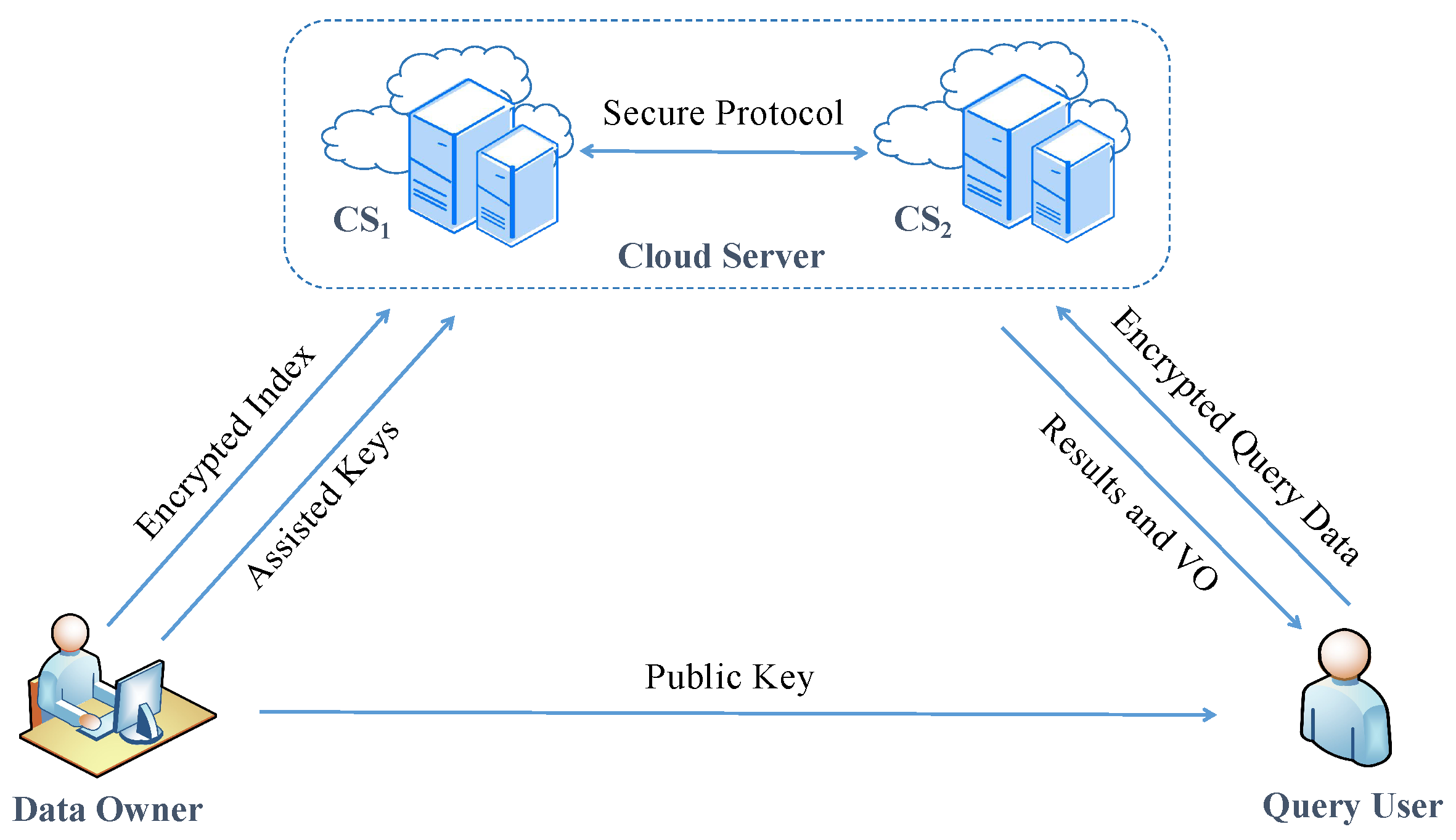
2.1. System Architecture and Threat Models

Following the setup of prior verifiable designs, our kNN query system over a cloud dataset, as illustrated in Figure 1, involves four entities: the data owner (DO), the query user (QU), and two cloud servers (CS₁ and CS₂). The DO possesses a large-scale spatial dataset $\mathcal{D}=\{\mathcal{D}\left[i\right]=(i,P_i)|i\in \left[n\right]\}$, and the QU issues a kNN query to the DO’s dataset. Due to limited storage and computing resources, the DO offloads the storage and associated computation tasks to the cloud servers while maintaining the privacy of the dataset. CS₁ and CS₂ are two non-colluding, resource-abundant, yet potentially untrusted cloud servers. To protect the privacy of the spatial dataset and support efficient kNN search operations, the DO must determine an appropriate blinding method and an efficient data structure to encrypt and organize the dataset $\mathcal{D}$. Also, the design should ensure that the QU can verify the integrity and correctness of the cloud returned query result. Formally, the framework of the privacy-preserving publicly verifiable kNN query scheme, denoted as PVkNN = (Setup, DSEnc, QuEnc, Search, Verify, ResDec), consists of the following six algorithms:

Figure 1. The system model.

• $\{PK,SK\}\leftarrow \mathbf{Setup}(1^{\lambda },n)$: Given a security parameter $\lambda$ and dataset size n, this algorithm generates the public key $PK$ and the secret key $SK$.
• $\{\mathcal{ED}\}\leftarrow \mathbf{DSEnc}(\mathcal{D},PK,SK)$: On inputting the dataset $\mathcal{D}$, the public key $PK$, and the secret key $SK$, the DO encrypts the dataset $\mathcal{D}$ into a ciphertext dataset $\mathcal{ED}=\{ED[i]|i\in \mathcal{I}\}$, where $\mathcal{I}$ denotes the label set.
• $\{Q^{\prime }\}\leftarrow \mathbf{QuEnc}(Q,PK)$: On inputting the query data point Q and the public key $PK$, this algorithms generates the encrypted query point $Q^{\prime }$.
• $\{{\mathcal{R}}^{\prime },\mathcal{VO}\}\leftarrow \mathbf{Search}(Q^{\prime },\mathcal{ED},PK)$: On inputting the encrypted query ${\sigma }_i$, the encrypted dataset $\mathcal{ED}$, and the public key $PK$, the search algorithm finds the query result ${\mathcal{R}}^{\prime }$ and the associated proof $\mathcal{VO}$.
• $\{\delta \}\leftarrow \mathbf{Verify}(Q,{\mathcal{R}}^{\prime },\mathcal{VO},PK)$: On inputting the encrypted query $Q^{\prime }$, the query result ${\mathcal{R}}^{\prime }$, the proof $\mathcal{VO}$, and the key pair $(PK,SK)$, the verification algorithm checks whether ${\mathcal{R}}^{\prime }$ is authentic and complete, producing an output $\delta \in \{True,False\}$.
• $\{\gamma \}\leftarrow \mathbf{ResDec}(Q,{\mathcal{R}}^{\prime },SK,\delta )$: With the query Q, the query result $\mathcal{R}$, the secret key $SK$ and the indicator $\delta$, if $\delta =True$, this algorithm decrypts the returned result ${\mathcal{R}}^{\prime }$ and recovers the set $\gamma =\mathcal{R}$ of k-nearest neighbors to Q. Otherwise, it rejects ${\mathcal{R}}^{\prime }$ and outputs $\gamma =\perp$.

In this kNN query system, the security threat mainly comes from untrustworthy cloud servers or malicious queriers. In our design, we consider the following three threat behaviors: (1) the cloud servers are curious and may attempt to infer confidential information, such as the dataset, the query access pattern, and the query result; (2) the cloud servers are malicious and may deliberately tamper with the query result for financial incentives; and (3) the querier is malicious and may forge a false query result and attribute it to the cloud servers.

Remark 1.

It should be noted that the two-non-colluding cloud servers framework is reasonable in practice. For well-established cloud service providers such as Amazon AWS, Microsoft Azure, or Huawei Cloud, it is highly unlikely that any two of these companies would collude to damage their invaluable reputations. Also, this setup has been extensively employed in secure kNN query scenarios [3,4,5,7,8,9,22,25].

2.2. Design Goals

Considering our system architecture and threat models, we aim to design a secure and efficient kNN query protocol. Specifically, our design should meet the four requirements outlined below.

2.2.1. Correctness

Generally, correctness means that if the cloud servers perform the specified computation task, the design should ensure that an honest querier can finally obtain the k-nearest neighbors to his/her query data point. The formal definition is presented below.

Definition 1 (Correctness).

A $\mathbf{PV}\mathit{k}\mathbf{NN}$ scheme is correct if, for any given security parameter λ, $\{PK,SK\}$$\leftarrow \mathit{Setup}(1^{\lambda },n)$, $\{\mathcal{ED}\}\leftarrow \mathbf{DSEnc}(\mathcal{D},PK,SK)$, $\{Q^{\prime }\}\leftarrow \mathit{QuEnc}(Q,PK)$, and $\{{\mathcal{R}}^{\prime },\mathcal{VO}\}\leftarrow \mathit{Search}(Q^{\prime },\mathcal{ED},PK)$ are honestly performed, the probability

$$\begin{array}{c}\hfill \mathrm{Pr}[\{\delta =True\}\leftarrow \mathit{Verify}(Q^{\prime },{\mathcal{R}}^{\prime },\mathcal{VO},PK)\wedge \{\gamma =\mathcal{R}\}\leftarrow \mathit{ResDec}(Q,{\mathcal{R}}^{\prime },SK,\delta )]\ge 1-\mathrm{negl}(\lambda ),\end{array}$$

where $\mathrm{negl}(\lambda )$ is a negligible function of λ.

2.2.2. Public Verifiability

In the context of verifiable kNN queries, verifiability refers to the ability to verify the authenticity and completeness of the query results returned by the cloud server. Specifically, this involves confirming whether the data in the query result was indeed uploaded by the DO and whether it corresponds precisely to the ciphertext of the k-nearest neighbors to the query point. Verification is considered private if it requires private keys, meaning that only the designated user who possesses the private keys can perform the verification [30,31]. Conversely, verification is public if it relies on public keys and can be performed by any entity [32,33,34]. Clearly, compared to private verifiability, public verifiability provides a more transparent verification mechanism. When disputes arise between the querier and the cloud server regarding the query results, public verifiability ensures the prompt resolution of such conflicts. Here, we define public verifiability using a private-key-independent verification algorithm called Verify, which guarantees that the probability of a cloud server successfully deceiving a verifier into accepting an incorrect result—either inauthentic or incomplete—is negligible. The formal definition is presented below.

${\mathrm{Exp}}_{\mathcal{A}}^{\mathrm{PV}}[\prod ,\lambda ,n]:$

$\{PK,SK\}\leftarrow \mathbf{Setup}(1^{\lambda },n)$

$\{\mathcal{ED}\}\leftarrow \mathbf{DSEnc}(\mathcal{D},PK,SK)$

$\mathbf{For}a=0\mathbf{to}t-1:$

$Q_a\leftarrow \mathcal{A}(PK,\mathcal{ED},Q_0,\cdots ,Q_{a-1})$

$Q_a^{\prime }\leftarrow \mathbf{QuEnc}(Q_a,PK)$

$\{{\mathcal{R}}_a,{\mathcal{VO}}_a\}\leftarrow \mathbf{Search}(Q_a^{\prime },ED,PK)$;

$Q\leftarrow \mathcal{A}(PK,\mathcal{ED},{(Q_a,Q_a^{\prime },{\mathcal{R}}_a^{\prime },{\mathcal{VO}}_a)}_{0\le a\le t-1});$

$Q^{\prime }\leftarrow \mathbf{QuEnc}(Q,PK)$

$\{{\mathcal{R}}^{\prime },\mathcal{VO}\}\leftarrow \mathcal{A}(PK,\mathcal{ED},Q,Q^{\prime },{(Q_a,Q_a^{\prime },{\mathcal{R}}_a,{\mathcal{VO}}_a)}_{0\le a\le t-1})$;

$\{\delta \}\leftarrow \mathbf{Verify}(Q,{\mathcal{R}}^{\prime },\mathcal{VO},PK);$

$\{\gamma \}\leftarrow \mathbf{ResDec}(Q,{\mathcal{R}}^{\prime },SK,\delta );$

$\mathbf{If}\delta =True\mathbf{and}\gamma \ne \mathcal{R}:$

$\mathrm{output}1;$

$\mathbf{else}$

$\mathrm{output}0;$

Definition 2 (Public Verifiability).

Let $\mathsf{\Pi }$ be a $\mathbf{PV}\mathit{k}\mathbf{NN}$ protocol, and let $\mathcal{A}(•)$ be a probabilistic polynomial-time (PPT) machine. We say that protocol $\mathsf{\Pi }$ is publicly verifiable if

$$Ad{v}_{\mathcal{A}}^{\mathrm{PV}}\left(\Pi ,\lambda ,n\right)\le negl(\lambda ),$$

where $Ad{v}_{\mathcal{A}}^{\mathrm{PV}}\left(\Pi ,\lambda ,n\right)=\mathrm{Pr}\left[{\mathrm{Exp}}_{\mathcal{A}}^{\mathrm{PV}}\left[\Pi ,\lambda ,n\right]=1\right]$.

2.2.3. Privacy

Our design aims to protect the privacy of the following information: the dataset, the query data, the query result, and query access pattern. The following privacy aspects are considered:

• Dataset privacy. Cloud servers cannot obtain any valuable information about the plaintext data in the dataset $\mathcal{D}$.
• Query data privacy. The QU’s query data should not be revealed to cloud servers.
• Query result privacy. Apart from the QU, other participants cannot learn the plaintext query result.
• Access pattern privacy. The identifiers corresponding to the k-nearest neighbors of the query point should not be revealed to the QU and the cloud servers (to prevent any inference attacks) [8,9,22].

In our analysis, we establish the privacy of our design by demonstrating the indistinguishability between the simulation model and the real model.

2.2.4. Efficiency

High efficiency is a generic requirement for any practical protocol. Under the premise of ensuring security, the design should reduce each participant’s computational and communication overheads as much as possible. Specifically, we should design an efficient index structure to support frequent query operations.

3. Preliminaries

3.1. Notations

For ease of description, we describe the frequently used notations in Table 2.

Table 2. Notations.

Notation	Description
$\rho$	a permutation function
$\mathcal{D}$	the plaintext spatial dataset
$\mathcal{ED}$	the ciphertext spatial dataset
$LCM(a,b)$	the least common multiple of two integers a and b
Q	$Q=(x_q,y_q)$ is the query data point
$i{d}_{\min }^{(j)}$	the index of the jth nearest neighbor to Q
$P_{i{d}_{\min }^{(j)}}$	$P_{i{d}_{\min }^{(j)}}=(x_{i{d}_{\min }^{(j)}},y_{i{d}_{\min }^{(j)}})$ denotes the jth
	nearest neighbor to Q
$VRV(P_{i{d}_{\min }^{(j)}})$	the set of Voronoi-relevant vectors of $P_{i{d}_{\min }^{(j)}}$
$\mathcal{H}(·)$	a cryptographic hash function
$\mathbf{Sig}(·)$	a DSA signature
N	a large integer that is the product of two
	prime numbers p and q
${\mathbb{Z}}_{N^2}^{★}$	the multiplicative group of the residue
	class modulo $N^2$
${\mathbb{Z}}_N^{★}$	the residue class ring modulo N
$x||y$	the concatenation of two numbers x and y
$\lfloor x\rfloor$	the greatest integer no larger than x
$\left[n\right]$	the set $\{0,\cdots ,n-1\}$
$\left[m\right]$	the set $\{0,\cdots ,m-1\}$
$\mathrm{negl}(·)$	a negligible function of some input parameter

3.2. Permutation

Given a natural number $m>0$, mathematically, a permutation $\rho$ is a bijection over the set $\{0,1,\cdots ,m-1\}$. Generally, it can be represented as

$$\left(\begin{array}{cccc}0& 1& \cdots & m-1\\ \rho (0)& \rho (1)& \cdots & \rho (m-1)\end{array}\right),$$

where $(\rho (0),\rho (1),\cdots ,\rho (m-1))$ is some rearrangement of $(0,1,\cdots ,m-1)$. For some m-tuple $v=(v_0,v_1,\cdots ,v_{m-1})$, we define $\rho (v)=\left(v_{\rho (0)},v_{\rho (1)},\cdots ,v_{\rho (m-1)}\right)$.

3.3. Paillier’s Additively Homomorphic Cryptosystem

The well-known Paillier additively homomorphic cryptosystem [35] was proposed by Paillier in 1999. For some message $m\in {\mathbb{Z}}_N$, its encryption function E is denoted as $c=E(m,r)={(1+N)}^m\times r^N\mathrm{mod}{N}^2,$ where N, which is public, is the product of two large prime numbers p and q, and $r\in {\mathbb{Z}}_N^{★}$ is randomly chosen. The decryption function D with the secret key $sk=\lambda (N)=LCM(p-1,q-1)$ is

$$m={\displaystyle \frac{c^{\lambda (N)}\mathrm{mod}{N}^2-1}{N}}·\lambda {(N)}^{-1}\mathrm{mod}N.$$

The Paillier cryptographic system exhibits the following properties:

• Homomorphic addition: The decrypted product of two ciphertexts equals the sum of their corresponding plaintexts, and the decrypted kth power of a ciphertext equals the product of k and its corresponding plaintext.

  $$\begin{array}{cc}\hfill & D\left(E(x_0)E(x_1)\mathrm{mod}{N}^2\right)=x_0+x_1\mathrm{mod}N,\hfill \\ \hfill & D\left(E{(x)}^k\mathrm{mod}{N}^2\right)=kx\mathrm{mod}N.\hfill \end{array}$$
• Semantic security: If the decisional composite residuosity problem is hard, then the Paillier cryptosystem is $\mathcal{CPA}$-secure.

3.4. Digital Signature Algorithm DSA

The Digital Signature Algorithm (DSA) is a standard algorithm for digital signatures and is a public-key cryptosystem based on the discrete logarithm problem [36]. For two large prime numbers p and q satisfying $q\mid p-1$, let $g\in {\mathbb{Z}}_p^{★}$ be an element of order q, and $y=g^x\mathrm{mod}p$ for some randomly chosen $x\in {\mathbb{Z}}_q^{★}$. Then, the signature key is $sk=\{x\}$, and the verification key is $pk=\{y\}$. For a message m, its signature is $\mathbf{Sig}(m)=(r,s)$, where, for some randomly chosen $k\in {\mathbb{Z}}_q^{★}$,

$$\begin{array}{c}\hfill r=(g^k\mathrm{mod}p)\mathrm{mod}q,s=k^{-1}(\mathcal{H}(m)+xr)\mathrm{mod}q,\end{array}$$

and $\mathcal{H}(·)$ is a public hash function. Given $(m,r,s)$, the verification algorithm $\{0,1\}\leftarrow \mathbf{Ver}(m,r,s)$ proceeds as follows: (1) Verify $r,s\in {\mathbb{Z}}_q^{★}$. (2) Calculate $w=s^{-1}\mathrm{mod}q$, $u_1=w\mathcal{H}(m)\mathrm{mod}q$, $u_2=wr\mathrm{mod}q$, and $v=(g^{u_1}{y}^{u_2}\mathrm{mod}p)\mathrm{mod}q$. (3) The algorithm outputs “1” (the signature is valid) if $v=r$. Otherwise, it outputs “0”.

3.5. Voronoi Diagram

Given a dataset $\mathcal{D}$ consisting of n points $\{P_0,\cdots ,P_{n-1}\}$ in the plane, the Voronoi region $Vor(P_i)$ of the point $P_i\in \mathcal{D}$ refers to the set of all points in the plane closer to $P_i$ than to any other point in $\mathcal{D}$. Precisely,

$$Vor(P_i)=\{\mathbf{x}\in {\mathbb{R}}^2|\parallel \mathbf{x}-{\mathbf{P}}_i\parallel \le \parallel \mathbf{x}-{\mathbf{P}}_{\mathbf{j}}\parallel ,\forall j\ne i\}.$$

(1)

Equivalently, for any $j\ne i$, let $H_{ij}=\{\mathbf{x}\in {\mathbb{R}}^2|\parallel \mathbf{x}-{\mathbf{P}}_i\parallel \le \parallel \mathbf{x}-{\mathbf{P}}_{\mathbf{j}}\parallel \}$ denote the half-plane, and we have $Vor(P_i)={\cap }_{j\ne i}{H}_{ij}$. The point $P_j$ is called a Voronoi-relevant vector of $P_i$ if and only if $Vor(P_j)$ and $Vor(P_i)$ share a boundary line. The set of these Voronoi-relevant vectors is generally denoted as $VRV(P_i)$.

Lemma 1

([37]). Given a dataset $\mathcal{D}=\{P_0,\cdots ,P_{n-1}\}$ and a query point Q, the nearest neighbor of the query point Q is P if and only if $Q\in Vor(P)$.

Lemma 2

([38]). Let $P_1,P_2,\cdots ,P_k$ be the k $(k\ge 2)$-nearest neighbors of a given query point Q. Then, $P_k\in VRV(P_1)\cup VRV(P_2)\cup \cdots \cup VRV(P_{k-1})$.

3.6. Data Packing with Paillier’s Cryptosystem

For a large-scale dataset, to encrypt and decrypt each data point item by item is time-consuming. To improve encryption/decryption efficiency, Liu et al. [39] introduced a data-packing encryption/decryption technique. Here, we present their design with Paillier’s cryptosystem. For $\lambda$$\sigma$-bits integers $x_1,x_2,\cdots ,x_{\lambda }$ with $2^{\sigma \lambda }<N$, unlike traditional methods that encrypt them into $E(x_1),E(x_2),\cdots ,E(x_{\lambda })$ item by item, the data-packing technique encrypts them into a single ciphertext, which contains the following four algorithms:

• Data packing $⟨x_1|x_2|\cdots |x_{\lambda }⟩\leftarrow \mathbf{Pack}(x_1,\cdots ,x_{\lambda })$:
  $⟨x_1|x_2|\cdots |x_{\lambda }⟩={\sum }_{i=1}^{\lambda }{x}_i{2}^{\sigma (\lambda -i)}.$
• Data encryption $c\leftarrow \mathbf{DataEnc}(⟨x_1|x_2|\cdots |x_{\lambda }⟩)$:
  $c=E(x_1|x_2|\cdots |x_{\lambda })=E({\sum }_{i=1}^{\lambda }{x}_i{2}^{\sigma (\lambda -i)}).$
• Data decryption $x\leftarrow \mathbf{DataDec}(c)$:
  $x=D(c).$
• Data unpacking $(x_1,x_2,\cdots ,x_{\lambda })\leftarrow \mathbf{Unpack}(x)$: $x_{\lambda }={\mathrm{lsb}}_{\sigma }(x),x_{\lambda -i}={\mathrm{lsb}}_{(i\sigma +1)\to (i+1)\sigma }(x)$ for $i=1,\cdots ,\lambda -1,$ where ${\mathrm{lsb}}_{(i\sigma +1)\to (i+1)\sigma }(x)$ denotes the binary bits between the $(i\sigma +1)$th position and the $(i+1)\sigma$th position of x counting from the least significant bit.

The correctness of the data decryption follows the fact that, since $2^{\lambda \sigma }<N$,

$$\begin{array}{c}\hfill D(c)=D(E(\sum _{i=1}^{\lambda }{x}_i{2}^{\sigma (\lambda -i)}))=\sum _{i=1}^{\lambda }{x}_i{2}^{\sigma (\lambda -i)}\mathrm{mod}N=\sum _{i=1}^{\lambda }{x}_i{2}^{\sigma (\lambda -i)}=x.\end{array}$$

The condition $2^{\lambda \sigma }<N$ is critical to guarantee the equivalence

$$\sum _{i=1}^{\lambda }{x}_i·2^{\sigma (\lambda -i)}\mathrm{mod}N=\sum _{i=1}^{\lambda }{x}_i·2^{\sigma (\lambda -i)},$$

as it ensures that the summation remains strictly smaller than the modulus N, thereby avoiding modular reduction. Also, if we know the ciphertext $E(x_i)$, we can get the ciphertext $E(x_1|x_2|\cdots |x_{\lambda })$ by using the homomorphic property, i.e.,

$$\begin{array}{c}\hfill E(x_1|\cdots |x_{\lambda })=E(\sum _{i=1}^{\lambda }{x}_i{2}^{\sigma (\lambda -i)})=\prod _{i=1}^{\lambda }E{(x_i)}^{2^{\sigma (\lambda -i)}}\mathrm{mod}{N}^2.\end{array}$$

4. Our Main Design

4.1. Design Intuition and Basic Idea

Inspired by [8,9], we adopt Paillier’s homomorphic cryptosystem to preserve the privacy of the dataset and the query data, as well as the “baby-step–giant-step” strategy to construct an efficient index data structure. Specifically, the spatial dataset is initially divided into several large rectangular regions, and each rectangle is further represented using a refined Voronoi diagram-based index. During the kNN search, we first perform a giant step to locate the target rectangular region, followed by a baby step to traverse the Voronoi diagram-based index and identify the individual points. To enable efficient search operations over the ciphertext dataset, we develop a series of secure protocols by integrating Paillier’s homomorphic encryption algorithm with the data-packing techniques, building upon previous designs. These protocols include the Secure Division Computation (SDC), Secure Grid Computation (SGC), Secure Nearest-Neighbor (SNN) search, and Secure Voronoi Cell Read (SCR) protocols, collectively enabling secure kNN queries. Since Paillier’s cryptosystem operates in a ring modulo a large integer and the data-packing technique is sensitive to parameter selection, we refine and tighten the previous designs to ensure correctness and optimize computational efficiency. This involves optimizing the index structure, improving parameter selection strategies, and addressing ambiguous or inaccurate descriptions. More importantly, previous designs lack support for public verifiability. In their approaches, the DO needs to send a secret verification key to the QU through a secure channel, or an additional Certified Authority (CA) is needed to generate and distribute keys through secure channels. To avoid the above-mentioned strong security assumption, as well as to prevent a malicious querier from forging a false query result and attributing it to the cloud servers, we integrate a public-key signature scheme with the Voronoi diagram-based index. This ensures both the authenticity and completeness of the query results while supporting public verifiability.

4.2. Our Main Outsourcing Protocol

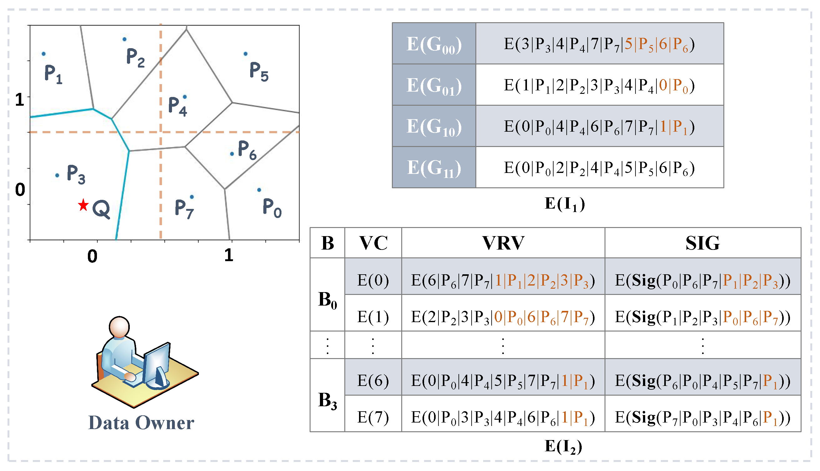
4.2.1. DO Dataset Preprocessing Stage

This stage, carried out by the DO, is a one-time process. Assume that the spatial dataset $\mathcal{D}=\{(i,P_i)|i\in \left[n\right]\}$, where each element comprises an identifier ($id$) i, and its corresponding point $P_i=(x_i,y_i)\in {\mathbb{R}}^2$. With loss of generality, we bound $x_i\in [0,X]$ and $y_i\in [0,Y]$ for any $i\in \left[n\right]$, and $\max \{X,Y,n-1\}<2^{\sigma }$. The aim of this stage is to construct two indexes (${\mathbf{I}}_1$ and ${\mathbf{I}}_2$) with the following steps:

• Given a natural number m of appropriate size, the DO divides the region $[0,X]\times [0,Y]$ into $m^2$ small rectangular regions $S_{st}=\left[{\displaystyle \frac{X}{m}}s,{\displaystyle \frac{X}{m}}(s+1)\right]\times \left[{\displaystyle \frac{Y}{m}}t,{\displaystyle \frac{Y}{m}}(t+1)\right]$ for $s,t\in \left[m\right]$.
• For each point $P_i$, the DO finds its Voronoi-relevant vectors

  $$\begin{array}{c}\hfill VRV(P_i)=\{(i_1,P_{i_1}),(i_2,P_{i_2}),\cdots ,(i_{{\ell }_i},P_{i_{{\ell }_i}})\}.\end{array}$$
• The DO constructs the index ${\mathbf{I}}_1=\{G_{st}|s,t\in \left[m\right]\}$, where $G_{st}=\{(s{t}_1,P_{s{t}_1}),(s{t}_2,P_{s{t}_2}),\cdots ,$$(s{t}_{{\lambda }_{st}},P_{s{t}_{{\lambda }_{st}}})\}$ refers to a subset of $\mathcal{D}$ and, for any point $P_{s{t}_u}\in G_{st}$, $Vor(P_{s{t}_u})\cap S_{st}\ne \varnothing$.
• The DO constructs the index ${\mathbf{I}}_2=\{⟨i,P_i,VRV(P_i)⟩|i\in \left[n\right]\}$.

4.2.2. System Setup Stage: $\mathbf{Setup}$

This stage is also performed by the DO and is a one-time task. Given a security parameter $\kappa$, the DO first invokes the key-generation algorithm in Paillier’s homomorphic cryptosystem to generate two random large prime numbers p and q with the same bit length $\kappa$ and calculates $N=pq,\lambda (N)=LCM(p-1,q-1)$. Then, the DO generates the signature-verification key pair $(sigk,verk)$ for the DSA. Finally, the DO publishes the public key $PK=\{p{k}_1=N,p{k}_2=verk\}$ and keeps the private key $SK=\{s{k}_1=\lambda (N),s{k}_2=sigk\}$ secret.

4.2.3. Dataset Encryption Stage: $\mathbf{DSEnc}$

This stage is performed by the DO and is a one-time task. As shown in the example illustrated in Figure 2, with the public key $p{k}_1$ for encryption and $s{k}_2$ for signature, the DO takes $w=\lceil \sqrt{n}\rceil$ and encrypts the dataset $\mathcal{D}$ into $\mathcal{ED}=(E({\mathbf{I}}_1),E({\mathbf{I}}_2))$ with

$$\begin{array}{c}\hfill E({\mathbf{I}}_1)=\left\{E\left(G_{st}\right)|s,t\in \left[m\right]\right\},E({\mathbf{I}}_2)=\left\{{\mathcal{B}}_j|j=0,1,\cdots ,⌈{\displaystyle \frac{n}{w}}⌉-1\right\}.\end{array}$$

Here, for $E({\mathbf{I}}_1)$,

$$\begin{array}{c}\hfill E(G_{st})=E\left(i_1^{(st)}|P_{i_1^{(st)}}|i_2^{(st)}|P_{i_2^{(st)}}|\cdots |i_{\lambda }^{(st)}|P_{i_{\lambda }^{(st)}}\right)=E\left(i_1^{(st)}|x_{i_1^{(st)}}|y_{i_1}^{(st)}|i_2^{(st)}|x_{i_2^{(st)}}|y_{i_2^{(st)}}|\cdots |i_{\lambda }^{(st)}|x_{i_{\lambda }^{(st)}}|y_{i_{\lambda }^{(st)}}\right)\end{array}$$

with $P_{i_u^{(st)}}=(x_{i_u^{(st)}},y_{i_u^{(st)}})$ for $u=1,\cdots ,\lambda$ and $\lambda ={\max }_{0\le s,t\le m-1}\{{\lambda }_{st}\}$. Specifically, if the number of points contained in some grid is less than $\lambda$, we can pad several random points chosen from $\mathcal{D}$. For $E({\mathbf{I}}_2)$,

$$\begin{array}{cc}\hfill {\mathcal{B}}_j& =\{(E(jw),E(VRV(P_{jw})),E(Sig(P_{jw}))),\cdots ,\hfill \\ \hfill & (E((j+1)w-1),E(VRV(P_{(j+1)w-1})),E(Sig(P_{(j+1)w-1})))\},\hfill \\ \hfill {\mathcal{B}}_{\lceil {\displaystyle \frac{n}{w}}\rceil -1}& =\{(E((\lceil {\displaystyle \frac{n}{w}}\rceil -1)w),E(VRV(P_{(\lceil {\displaystyle \frac{n}{w}}\rceil -1)w})),E(Sig(P_{(\lceil {\displaystyle \frac{n}{w}}\rceil -1)w}))),\cdots ,\hfill \\ \hfill & (E((\lceil {\displaystyle \frac{n}{w}}\rceil )w-1),E(VRV(P_{(\lceil {\displaystyle \frac{n}{w}}\rceil )w-1})),E(Sig(P_{(\lceil {\displaystyle \frac{n}{w}}\rceil )w-1})))\},\hfill \end{array}$$

are $\lceil {\displaystyle \frac{n}{w}}\rceil$ buckets, each bucket consisting of w three-tuples. Specifically, for the last bucket ${\mathcal{B}}_{\lceil {\displaystyle \frac{n}{w}}\rceil -1}$, we pad the subscripts $n,n+1,\cdots ,\lceil {\displaystyle \frac{n}{w}}\rceil -1$ with some random data points if it contains no more than w three-tuples. Moreover, for any $i\in \left[n\right]$, $E(VRV(P_i))=E(i_1|P_{i_1}|i_2|P_{i_2}|\cdots |i_L|P_{i_L}),E(Sig(P_i))=E(\mathbf{Sig}(P_i||P_{i_1}||\cdots ||P_{i_L}))$. Similarly, if the number of points contained in some $VRV(P_i)$ is less than $L=\max \{{\ell }_0,\cdots ,{\ell }_{n-1}\}$, we can pad several random points chosen from $\mathcal{D}$. Finally, the DO uploads $(\mathcal{ED},E(X/m),E(Y/m))$ to CS₁ and the private key $s{k}_1$ to CS₂.

Figure 2. An example of $\mathcal{ED}=(E({\mathbf{I}}_1),E({\mathbf{I}}_2))$ with the grid granularity $m=2$, $E({\mathbf{I}}_1)=\left\{E\left(G_{st}\right)|s,t=0,1\right\}$, and $E({\mathbf{I}}_2)=\left\{{\mathcal{B}}_j|j=0,1,2,3\right\}$. The points with red are padding records.

4.2.4. QU Query Encryption Stage: $\mathbf{QuEnc}$

This stage is performed by the QU. When the QU issues a kNN query request $Q=(x_q,y_q)$, he/she encrypts it into $E(Q)=(E(x_q),E(y_q))$ with the public key $p{k}_1$ and then queries CS₁ with $E(Q)$.

4.2.5. CS Search Stage: $\mathbf{Search}$

This stage is cooperatively performed by the two non-colluding cloud servers CS₁ and CS₂ and is a query-based one-time operation. Algorithm 1 presents the details. In general, this stage proceeds as follows:

Algorithm 1 kNN ($E_{pk}(\mathbf{I}),E_{pk}(X/m),E_{pk}(Y/m),E(Q),p{k}_1,s{k}_1$)

Input: ${\mathbf{CS}}_1:E_{pk}(\mathbf{I})=(E({\mathbf{I}}_1),E({\mathbf{I}}_2)),E_{pk}(X/m),E_{pk}(Y/m)),E(Q),pk,$CS2: the public-private key pair $(p{k}_1,s{k}_1)$

Output: Result sets ${\mathcal{R}}_1$, ${\mathcal{R}}_2$, and verification sets ${\mathcal{VO}}_1$, ${\mathcal{VO}}_2$

1: CS1 initializes two empty sets ${\mathcal{R}}_1\leftarrow \varnothing$, ${\mathcal{VO}}_1\leftarrow \varnothing$, CS2 initializes two empty sets ${\mathcal{R}}_2\leftarrow \varnothing$, ${\mathcal{VO}}_2\leftarrow \varnothing$    2: CS1 and CS2 jointly perform Algorithm 2: $(E(\lfloor {\displaystyle \frac{x_q}{X/m}}\rfloor ),E(\lfloor {\displaystyle \frac{y_q}{Y/m}}\rfloor ))\leftarrow \mathrm{SDC}(E(Q),(E(X/m),E(Y/m)),p{k}_1,s{k}_1)$    3: CS1 and CS2 jointly perform Algorithm 3: $E(G_{\widehat{s}\widehat{t}})\leftarrow$ SGC($E({\mathbf{I}}_1),E(\lfloor {\displaystyle \frac{x_q}{X/m}}\rfloor ),E(\lfloor {\displaystyle \frac{y_q}{Y/m}}\rfloor ),p{k}_1,s{k}_1$)    4: ${\mathbf{CS}}_1$ and CS2 jointly perform Algorithm 4: $(E(i{d}_{\min }^{(1)}),E(x_{i{d}_{\min }^{(1)}}),E(y_{i{d}_{\min }^{(1)}}))\leftarrow$ SNN($E(G_{\widehat{s}\widehat{t}}),E(Q),\perp ,p{k}_1,s{k}_1)$    5: CS1 generates three random number $r_1^{(1)},r_2^{(1)},r_3^{(1)}\in {\mathbb{Z}}_N$ and updates ${\mathcal{R}}_1\leftarrow {\mathcal{R}}_1\cup \{(r_2^{(1)},r_3^{(1)})\}$    6: CS1 calculates $(E(i{d}_{\min }^{(1)\prime }),E(x_{i{d}_{\min }^{(1)}}^{\prime }),E(y_{i{d}_{\min }^{(1)}}^{\prime }))\leftarrow (E(i{d}_{\min }^{(1)})\times E(r_1^{(1)}),E(x_{i{d}_{\min }^{(1)}})\times E(r_2^{(1)}),E(y_{i{d}_{\min }^{(1)}})\times E(r_3^{(1)}))$ and sends it to ${\mathbf{CS}}_2$    7: ${\mathbf{CS}}_2$ decrypts $(i{d}_{\min }^{(1)\prime },x_{i{d}_{\min }^{(1)}}^{\prime },y_{i{d}_{\min }^{(1)}}^{\prime })\leftarrow (D(E(i{d}_{\min }^{(1)\prime })),D(E(x_{i{d}_{\min }^{(1)}}^{\prime })),D(E(y_{i{d}_{\min }^{(1)}}^{\prime })))$ and updates ${\mathcal{R}}_2\leftarrow {\mathcal{R}}_2\cup \{(x_{i{d}_{\min }^{(1)}}^{\prime },y_{i{d}_{\min }^{(1)}}^{\prime })\}$    8: ${\mathbf{CS}}_1$ and CS2 jointly perform Algorithm 5: $(E(VRV(P_{i{d}_{\min }^{(1)}}),E(Sig(P_{i{d}_{\min }^{(1)}})))\leftarrow$ SCR($E({\mathbf{I}}_2),E(i{d}_{\min }^{(1)}),p{k}_1,s{k}_1)$    9: CS1 generates $3L+1$ random numbers $r_{4,1}^{(1)},r_{4,2}^{(1)},\cdots ,r_{4,3L}^{(1)},r_5^{(1)}\in {\mathbb{Z}}_N$, packs $r_{4,1}^{(1)}\sim r_{4,3L}^{(1)}$ into $r_0^{(1)}=⟨r_{4,1}^{(1)}|r_{4,2}^{(1)}|\cdots |r_{4,3L}^{(1)}⟩$ and updates ${\mathcal{VO}}_1\leftarrow {\mathcal{VO}}_1\cup \{((r_{4,2}^{(1)},r_{4,3}^{(1)}),\cdots ,(r_{4,3k-1}^{(1)},r_{4,3k}^{(1)}),\cdots ,(r_{4,3L-1}^{(1)},r_{4,3L}^{(1)}),r_5^{(1)})\}$   10: CS1 calculates $E(VRV{(P_{i{d}_{\min }^{(1)}})}^{\prime })\leftarrow E(VRV(P_{i{d}_{\min }^{(1)}}))\times E(r_0^{(1)}),E(Sig{(P_{i{d}_{\min }^{(1)}})}^{\prime })\leftarrow E(Sig(P_{i{d}_{\min }^{(1)}}))\times E(r_5^{(1)})$ and sends them to ${\mathbf{CS}}_2$   11: ${\mathbf{CS}}_2$ decrypts $(VRV{(P_{i{d}_{\min }^{(1)}})}^{\prime },Sig{(P_{i{d}_{\min }^{(1)}})}^{\prime })\leftarrow (D(E(VRV{(P_{i{d}_{\min }^{(1)}})}^{\prime })),D(E(Sig{(P_{i{d}_{\min }^{(1)}})}^{\prime })))$   12: ${\mathbf{CS}}_2$ unpacks $\{{i{d}_1^{(1)}}^{\prime },P_{{i{d}_1^{(1)}}^{\prime }}^{\prime },\cdots ,{i{d}_L^{(1)}}^{\prime },P_{{i{d}_L^{(1)}}^{\prime }}^{\prime }\}\leftarrow \mathbf{Unpack}(VRV{(P_{i{d}_{\min }^{(1)}})}^{\prime })$, where $P_{{i{d}_1^{(1)}}^{\prime }}^{\prime }=(x_{{i{d}_1^{(1)}}^{\prime }}^{\prime },y_{{i{d}_1^{(1)}}^{\prime }}^{\prime }),$$\cdots ,$$P_{{i{d}_L^{(1)}}^{\prime }}^{\prime }$$=(x_{{i{d}_L^{(1)}}^{\prime }}^{\prime },y_{{i{d}_L^{(1)}}^{\prime }}^{\prime })$.   13: ${\mathbf{CS}}_2$ updates ${\mathcal{VO}}_2\leftarrow {\mathcal{VO}}_2\cup \{(P_{{i{d}_1^{(1)}}^{\prime }}^{\prime },\cdots ,P_{{i{d}_L^{(1)}}^{\prime }}^{\prime },Sig{(P_{i{d}_{\min }^{(1)}})}^{\prime })\}$   14: for $j=2$ to k do   15:    ${\mathbf{CS}}_1$ and CS2 jointly perform Algorithm 4: $(E(i{d}_{\min }^{(j)}),E(x_{i{d}_{min}^{(j)}}),E(y_{i{d}_{\min }^{(j)}}))\leftarrow$ SNN $(\{E(VRV(P_{i{d}_{\min }^{(1)}})),\cdots ,$$E(VRV(P_{i{d}_{\min }^{(j-1)}})\},E(Q),\{E(i{d}_{\min }^{(1)}),\cdots ,E(i{d}_{\min }^{(j-1)})\},p{k}_1,s{k}_1)$   16:    ${\mathbf{CS}}_1$ generate three random numbers $r_1^{(j)},r_2^{(j)},r_3^{(j)}\in {\mathbb{Z}}_N$ and updates ${\mathcal{R}}_1\leftarrow {\mathcal{R}}_1\cup \{(r_2^{(j)},r_3^{(j)})\}$   17:    CS1 calculates $(E(i{d}_{\min }^{(j)\prime }),E(x_{i{d}_{\min }^{(j)}}^{\prime }),E(y_{i{d}_{\min }^{(j)}}^{\prime }))\leftarrow (E(i{d}_{\min }^{(j)})\times E(r_1^{(j)}),E(x_{i{d}_{\min }^{(j)}})\times E(r_2^{(j)}),E(y_{i{d}_{\min }^{(j)}})\times E(r_3^{(j)}))$ and sends it to ${\mathbf{CS}}_2$   18:    ${\mathbf{CS}}_2$ decrypts $(i{d}_{\min }^{(j)\prime },x_{i{d}_{\min }^{(j)}}^{\prime },y_{i{d}_{\min }^{(j)}}^{\prime })\leftarrow (D(E(i{d}_{\min }^{(j)\prime })),D(E(x_{i{d}_{\min }^{(j)}}^{\prime })),D(E(y_{i{d}_{\min }^{(j)}}^{\prime })))$ and updates ${\mathcal{R}}_2\leftarrow {\mathcal{R}}_2\cup \{(x_{i{d}_{\min }^{(j)}}^{\prime },y_{i{d}_{\min }^{(j)}}^{\prime })\}$   19:    ${\mathbf{CS}}_1$ and ${\mathbf{CS}}_2$ jointly perform Algorithm 5: $(E(VRV(P_{i{d}_{\min }^{(j)}}),E(Sig(P_{i{d}_{\min }^{(j)}})))\leftarrow$ SCR($E({\mathbf{I}}_2),E(i{d}_{\min }^{(j)}),p{k}_1,s{k}_1)$   20:    ${\mathbf{CS}}_1$ generates $3L+1$ random numbers $r_{4,1}^{(j)},r_{4,2}^{(j)},\cdots ,r_{4,3L}^{(j)},r_5^{(j)}\in {\mathbb{Z}}_N$, packs $r_{4,1}^{(j)}\sim r_{4,3L}^{(j)}$ into $r_0^{(j)}=⟨r_{4,1}^{(j)}|r_{4,2}^{(j)}|\cdots |r_{4,3L}^{(j)}⟩$ and updates ${\mathcal{VO}}_1\leftarrow {\mathcal{VO}}_1\cup \{(r_{4,2}^{(j)},r_{4,3}^{(j)},\cdots ,r_{4,3L}^{(j)},r_5^{(j)})\}$   21:    ${\mathbf{CS}}_1$ calculates $E(VRV{(P_{i{d}_{\min }^{(j)}})}^{\prime })\leftarrow E(VRV(P_{i{d}_{\min }^{(j)}}))\times E(r_0^{(j)})$, $E(Sig{(P_{i{d}_{\min }^{(j)}})}^{\prime })\leftarrow E(Sig(P_{i{d}_{\min }^{(j)}}))\times E(r_5^{(j)})$ and sends them to ${\mathbf{CS}}_2$   22:    ${\mathbf{CS}}_2$ decrypts $(VRV{(P_{i{d}_{\min }^{(j)}})}^{\prime },Sig{(P_{i{d}_{\min }^{(j)}})}^{\prime })\leftarrow (D(E(VRV{(P_{i{d}_{\min }^{(j)}})}^{\prime })),D(E(Sig{(P_{i{d}_{\min }^{(j)}})}^{\prime })))$   23:    ${\mathbf{CS}}_2$ unpacks $\{{i{d}_1^{(j)}}^{\prime },P_{{i{d}_j^{(1)}}^{\prime }}^{\prime },\cdots ,{i{d}_L^{(j)}}^{\prime },P_{{i{d}_L^{(j)}}^{\prime }}^{\prime }\}\leftarrow \mathbf{Unpack}(VRV{(P_{i{d}_{\min }^{(j)}})}^{\prime })$, where $P_{{i{d}_1^{(j)}}^{\prime }}^{\prime }=(x_{{i{d}_1^{(j)}}^{\prime }}^{\prime },y_{{i{d}_1^{(j)}}^{\prime }}^{\prime }),\cdots ,$$P_{{i{d}_L^{(j)}}^{\prime }}^{\prime }=$$(x_{{i{d}_L^{(j)}}^{\prime }}^{\prime },y_{{i{d}_L^{(j)}}^{\prime }}^{\prime })$   24:    ${\mathbf{CS}}_2$ updates ${\mathcal{VO}}_2\leftarrow {\mathcal{VO}}_2\cup \{(P_{{i{d}_1^{(j)}}^{\prime }}^{\prime },\cdots ,P_{{i{d}_L^{(j)}}^{\prime }}^{\prime },Sig{(P_{i{d}_{\min }^{(j)}})}^{\prime })\}$.   25: ${\mathbf{CS}}_1$ sends ${\mathcal{R}}_1=\{(r_2^{(j)},r_3^{(j)})|j=1,\cdots ,k\}$ and ${\mathcal{VO}}_1=\{((r_{4,2}^{(j)},r_{4,3}^{(j)}),\cdots ,(r_{4,3L-1},r_{4,3L}^{(j)}),r_5^{(j)})|j=1,\cdots ,k\}$ to QU   26: ${\mathbf{CS}}_2$ sends ${\mathcal{R}}_2=\{(x_{i{d}_{\min }^{(j)}}^{\prime },y_{i{d}_{\min }^{(j)}}^{\prime })|j=1,\cdots ,k\}$ and ${\mathcal{VO}}_2=\{(P_{{i{d}_1^{(j)}}^{\prime }}^{\prime },\cdots ,P_{{i{d}_L^{(j)}}^{\prime }}^{\prime },Sig{(P_{i{d}_{\min }^{(j)}})}^{\prime })|j=1,\cdots ,k\}$ to QU

(1)

With the inputs $E(Q)=(E(x_q),E(y_q))$, $(E(X/m)$, and $E(Y/m))$, and the public–private key pair $(p{k}_1,s{k}_1)$, cloud servers ${\mathbf{CS}}_1$ and ${\mathbf{CS}}_2$ interact with each other to calculate the ciphertexts $E(\lfloor {\displaystyle \frac{x_q}{X/m}}\rfloor )$ and $E(\lfloor {\displaystyle \frac{y_q}{Y/m}}\rfloor )$ using Algorithm 2.

(2)

With the inputs $E({\mathbf{I}}_1),E(\lfloor {\displaystyle \frac{x_q}{X/m}}\rfloor ),E(\lfloor {\displaystyle \frac{y_q}{Y/m}}\rfloor ),p{k}_1,$ and $s{k}_1$, cloud servers ${\mathbf{CS}}_1$ and ${\mathbf{CS}}_2$ collaborate to execute Algorithm 3, traversing $E({\mathbf{I}}_1)$ to locate the target grid $E(G_{\widehat{s}\widehat{t}})$ with $\widehat{s}=\lfloor {\displaystyle \frac{x_q}{X/m}}\rfloor ,\widehat{t}=\lfloor {\displaystyle \frac{y_q}{Y/m}}\rfloor$, which means that $Q\in G_{\widehat{s}\widehat{t}}$. The core idea of this algorithm is to determine $(\widehat{s},\widehat{t})$ based on verifying whether both $E(\lfloor {\displaystyle \frac{x_q}{X/m}}\rfloor )\times {(E(s))}^{N-1}=E(\lfloor {\displaystyle \frac{x_q}{X/m}}\rfloor -s)$ and $E(\lfloor {\displaystyle \frac{y_q}{Y/m}}\rfloor )\times {(E(t))}^{N-1}=E(\lfloor {\displaystyle \frac{y_q}{Y/m}}\rfloor -t)$ represent ciphertexts of 0 for some $s,t\in 0,\cdots ,m-1$. Note that $\lfloor {\displaystyle \frac{x_q}{X/m}}\rfloor -s$ may be negative; the parameter T ensures that $E(\lfloor {\displaystyle \frac{x_q}{X/m}}\rfloor )\times {(E(s))}^{N-1}\times E(T)=E(\lfloor {\displaystyle \frac{x_q}{X/m}}\rfloor -s+T)$ ensures that the results represents a ciphertext of a positive number.

Algorithm 2 SDC ($E(Q),(E(X/m),E(Y/m)),p{k}_1,s{k}_1$)

Input: ${\mathbf{CS}}_1$: $E(Q)=(E(x_q),E(y_q))$, $(E(X/m),E(Y/m))$ and a security parameter $\tau <\kappa -{\displaystyle \frac{\sigma }{2}}-1$, ${\mathbf{CS}}_2$: $p{k}_1,s{k}_1$.

Output: ${\mathbf{CS}}_1$ obtains the quotients $E(\lfloor {\displaystyle \frac{x_q}{X/m}}\rfloor )$ and $E(\lfloor {\displaystyle \frac{y_q}{Y/m}}\rfloor )$

1: ${\mathbf{CS}}_1$ generates two random numbers $r_1,r_2\in {\mathbb{Z}}_N$ with $\tau$ bits    2: ${\mathbf{CS}}_1$ calculates $x^{\prime }\leftarrow E{(x_q)}^{r_1}\times E{(X/m)}^{r_1{r}_2}$, $u^{\prime }\leftarrow E{(X/m)}^{r_1}$ and $y^{\prime }\leftarrow E{(y_q)}^{r_1}\times E{(Y/m)}^{r_1{r}_2}$, $v^{\prime }\leftarrow E{(Y/m)}^{r_1}$    3: ${\mathbf{CS}}_1$ sends $(x^{\prime },y^{\prime })$ and $(u^{\prime },v^{\prime })$ to ${\mathbf{CS}}_2$    4: ${\mathbf{CS}}_2$ decrypts $(x,y)\leftarrow (D(x^{\prime }),D(y^{\prime }))$ and $(u,v)\leftarrow (D(u^{\prime }),D(v^{\prime }))$    5: ${\mathbf{CS}}_2$ calculates the quotients $d_x=\lfloor {\displaystyle \frac{x}{u}}\rfloor$ and $d_y=\lfloor {\displaystyle \frac{y}{v}}\rfloor$    6: ${\mathbf{CS}}_2$ encrypts $d_x^{\prime }\leftarrow E(d_x)$ and $d_y^{\prime }\leftarrow E(d_y)$ with $pk$    7: ${\mathbf{CS}}_2$ sends $(d_x^{\prime },d_y^{\prime })$ to ${\mathbf{CS}}_1$    8: ${\mathbf{CS}}_1$ calculates the quotients $E(\lfloor {\displaystyle \frac{x_q}{X/m}}\rfloor )=d_x^{\prime }\times E{(r_2)}^{N-1}$ and $E(\lfloor {\displaystyle \frac{y_q}{Y/m}}\rfloor )=d_y^{\prime }\times E{(r_2)}^{N-1}$

Algorithm 3 SGC ($E({\mathbf{I}}_1),E(\lfloor {\displaystyle \frac{x_q}{X/m}}\rfloor ),E(\lfloor {\displaystyle \frac{y_q}{Y/m}}\rfloor ),p{k}_1,s{k}_1$)

Input: ${\mathbf{CS}}_1$: $E({\mathbf{I}}_1)=\{E(G_{st})|s,t\in \left[m\right]\},$$E(\lfloor {\displaystyle \frac{x_q}{X/m}}\rfloor ),$$E(\lfloor {\displaystyle \frac{y_q}{Y/m}}\rfloor )$, $p{k}_1$ and security parameters $\tau ,{\sigma }^{\prime }$ satisfying $2^{\tau +\sigma }<2^{{\sigma }^{\prime }},2^{{\sigma }^{\prime }m}<N$, ${\mathbf{CS}}_2$: $p{k}_1,s{k}_1,m$

Output: the grid $E(G_{\widehat{s}\widehat{t}})$ with $\widehat{s}=\lfloor {\displaystyle \frac{x_q}{X/m}}\rfloor$ and $\widehat{t}=\lfloor {\displaystyle \frac{y_q}{Y/m}}\rfloor$

1: ${\Delta }_x\leftarrow \varnothing ,{\Delta }_y\leftarrow \varnothing ,{\Gamma }^{\prime }\leftarrow \varnothing ,M\leftarrow \varnothing$

2: for $j=0$ to $m-1$ do

3:    ${\mathbf{CS}}_1$ generates random numbers $r_{xj},r_{yj}\in {\mathbb{Z}}_N$ with $\tau$ bits and a random number $T\ge m$

4:     ${\mathbf{CS}}_1$ calculates $${\Delta }_{xj}\leftarrow {\left(E(\lfloor {\displaystyle \frac{x_q}{X/m}}\rfloor )\times E{(j)}^{N-1}\times E(T)\right)}^{r_{xj}},{\Delta }_{yj}\leftarrow {\left(E(\lfloor {\displaystyle \frac{y_q}{Y/m}}\rfloor )\times E{(j)}^{N-1}\times E(T)\right)}^{r_{yj}}$$

5: ${\Delta }_x\leftarrow ({\Delta }_{x0},{\Delta }_{x1},\cdots ,{\Delta }_{x(m-1)}),{\Delta }_y\leftarrow ({\Delta }_{y0},{\Delta }_{y1},$$\cdots ,$${\Delta }_{y(m-1)})$

6: for $s=0$ to $m-1$ do

7:         for $t=0$ to $m-1$ do

8:                  ${\mathbf{CS}}_1$ generates a random numbers $r_{st}$ and calculates $E(r_{st})$

9:                  ${\mathbf{CS}}_1$ computes $E(G_{st}^{\prime })\leftarrow E(G_{st})\times E(r_{st})$

10: $E(G^{\prime })\leftarrow {(E(G_{st}^{\prime }))}_{0\le s,t\le m-1}$

11: ${\mathbf{CS}}_1$ permutes the vectors ${\Delta }_x,{\Delta }_y$ and grid $E(G^{\prime })$ with two random permutations ${\rho }_1,{\rho }_2$:

12: ${\Delta }_x^{\prime }={\rho }_1({\Delta }_x)=({\Delta }_{x{\rho }_1(0)},{\Delta }_{x{\rho }_1(1)},\cdots ,{\Delta }_{x{\rho }_1(m-1)}),$${\Delta }_y^{\prime }={\rho }_2({\Delta }_y)=({\Delta }_{y{\rho }_2(0)},{\Delta }_{y{\rho }_2(1)},\cdots ,{\Delta }_{y{\rho }_2(m-1)}),$

13: ${\Gamma }^{\prime }={\rho }_2({\rho }_1(E(G^{\prime })))={(E(G_{{\rho }_1(s){\rho }_2(t)}^{\prime }))}_{0\le s,t\le m-1}$

14: ${\mathbf{CS}}_1$ packs ${\Delta }_x^{\prime },{\Delta }_y^{\prime }$, i.e., calculates $v_x^{\prime }\leftarrow {\prod }_{i=0}^{m-1}{\Delta }_{x{\rho }_1(i)}^{2^{{\sigma }^{\prime }(m-(i+1))}},v_y^{\prime }\leftarrow {\prod }_{i=0}^{m-1}{\Delta }_{y{\rho }_2(i)}^{2^{{\sigma }^{\prime }(m-(i+1))}}$ and sends $v_x^{\prime },v_y^{\prime },{\Gamma }^{\prime },T$ to ${\mathbf{CS}}_2$

15: ${\mathbf{CS}}_2$ decrypts and unpacks $v_x^{\prime }$ and $v_y^{\prime }$: $(v_{x{\rho }_1(0)},$$\cdots ,$$v_{x{\rho }_1(m-1)})\leftarrow D(v_x^{\prime }),(v_{y{\rho }_2(0)},$$\cdots ,v_{y{\rho }_2(m-1)})\leftarrow D(v_y^{\prime })$

16: for $s=0$ to $m-1$ do

17:         for $t=0$ to $m-1$ do

18:                 if $v_{x{\rho }_1(s)}\mathrm{mod}T=0$ and $v_{y{\rho }_2(t)}\mathrm{mod}T=0$

19:

20:                      ${\Gamma }^{\prime }\leftarrow {\Gamma }_{{\rho }_1(s){\rho }_2(t)}^{\prime }=E\left(G_{{\rho }_1(s){\rho }_2(t)}^{\prime }\right),M_{st}\leftarrow E(1)$

21:

22:                   else $M_{st}\leftarrow E(0)$

23: ${\mathbf{CS}}_2$ sends ${\Gamma }^{\prime }$ and $M={\left(M_{st}\right)}_{0\le s,t\le m-1}$ to ${\mathbf{CS}}_1$

24: ${\mathbf{CS}}_1$ permutes the matrix M with ${\rho }_1,{\rho }_2$: $M^{\prime }\leftarrow {\rho }_1^{-1}({\rho }_2^{-1}(M))$

25: ${\mathbf{CS}}_1$ calculates $E(r)\leftarrow {\prod }_{s=0}^{m-1}{\prod }_{t=0}^{m-1}{(M_{st}^{\prime })}^{r_{st}}$

26: ${\mathbf{CS}}_1$ gets the target grid $E(G_{\widehat{s}\widehat{t}})$ containing the query point: $E(G_{\widehat{s}\widehat{t}})\leftarrow {\Gamma }^{\prime }\times E{(r)}^{N-1}$

(3)

After identifying the correct grid $E(G_{\widehat{s}\widehat{t}})$, cloud servers CS1 and CS2 jointly execute Algorithm 4 to search within the grid $G\widehat{s}\widehat{t}$ in ciphertext form and locate the ciphertext ($E(i{d}^{(1)}min),E(x_{i{d}_{min}^{(1)}}),E(y_{i{d}_{min}^{(1)}})$) corresponding to the nearest neighbor to Q, where $(i{d}_{min}^{(1)},P_{i{d}_{min}^{(1)}}=(x_{i{d}_{min}^{(1)}},y_{i{d}_{min}^{(1)}}))\in G_{\widehat{s}\widehat{t}}$. It is worth noting that Algorithm 4 can trivially be adapted to handle scenarios where the input includes multiple packed ciphertext datasets and multiple ciphertext $id$ values. Specifically, the input format is $(\{E(G^{(1)}),\cdots ,E(G^{(\alpha )})\},E(Q),\{E(i{d}_1),E(i{d}_2),\cdots ,$$E(i{d}_{\beta })\},p{k}_1,s{k}_1)$, and the output is the ciphertext $(E(i{d}_{min}),E(x_{i{d}_{min}}),E(y_{i{d}_{min}}))$, where $P_{i{d}_{min}}=(x_{i{d}_{min}},y_{i{d}_{min}})\in G^{(1)}\cup \cdots \cup G^{(\alpha )}$ represents the nearest-neighbor point to Q, with the constraint that $i{d}_{\min }\notin \{i{d}_1,i{d}_2,\cdots ,i{d}_{\beta }\}$.

Algorithm 4 SNN ($E(G_{\widehat{s}\widehat{t}}),E(Q),E(id),p{k}_1,s{k}_1$)

Input: ${\mathbf{CS}}_1$: $E(Q)=(E(x_q),E(y_q))$, $E(G_{\widehat{s}\widehat{t}})$ and $E(id)$, ${\mathbf{CS}}_2$: the private key $s{k}_1$

Output: ($E(i{d}_{\min }),E(x_{i{d}_{\min }}),E(y_{i{d}_{\min }})$): the ciphertext of the nearest neighbor $(i{d}_{\min },P_{i{d}_{\min }}=(x_{i{d}_{\min }},y_{i{d}_{\min }}))\in G_{\widehat{s}\widehat{t}}$ to Q with $i{d}_{\min }\ne id$

1: ${\mathbf{CS}}_1$ generates $3\lambda +1$ random numbers $r_0,r_1,\cdots ,r_{3\lambda }\in {\mathbb{Z}}_N$    2: ${\mathbf{CS}}_1$ packs $r_1\sim r_{3\lambda }$ into ${\Phi }_0=⟨r_1|r_2|\cdots |r_{3\lambda }⟩$, packs $r_2,r_3,r_5,r_6,\cdots ,r_{3\lambda -1},r_{3\lambda }$ into ${\Phi }_1=⟨r_2|r_3|\cdots |r_{3\lambda -1}|r_{3\lambda }⟩$ and packs $r_1,r_4,r_7,\cdots ,r_{3\lambda -2}$ into ${\Phi }_2=⟨r_1|r_4|\cdots |r_{3\lambda -2}⟩$    3: ${\mathbf{CS}}_1$ calculates $v_0^{\prime }\leftarrow {(E(G_{\widehat{s}\widehat{t}})\times E({\Phi }_0))}^{r_0}$    4: ${\mathbf{CS}}_1$ calculates $E(Q^{\prime })\leftarrow E(x_q|y_q|x_q|y_q|\cdots |x_q|y_q)=E{(x_q)}^{2^{\sigma (2\lambda -1)}}$$E{(y_q)}^{2^{\sigma (2\lambda -2)}}\cdots$$E{(x_q)}^{2^{\sigma }}E{(y_q)}^{2^0}$    5: ${\mathbf{CS}}_1$ calculates $v_1^{\prime }\leftarrow {(E(Q^{\prime })\times E({\Phi }_1))}^{r_0}$    6: ${\mathbf{CS}}_1$ calculates $E(i{d}^{\prime })\leftarrow E(id|id|id|id|\cdots |id|id)=E{(id)}^{2^{\sigma (\lambda -1)}}E{(id)}^{2^{\sigma (\lambda -2)}}\cdots$$E{(id)}^{2^{\sigma }}E{(id)}^{2^0}$    7: ${\mathbf{CS}}_1$ calculates $v_2^{\prime }\leftarrow {(E(i{d}^{\prime })\times E({\Phi }_2))}^{r_0}$    8: ${\mathbf{CS}}_1$ sends $v_0^{\prime },v_1^{\prime },v_2^{\prime }$ to ${\mathbf{CS}}_2$    9: ${\mathbf{CS}}_2$ decrypts $v_0\leftarrow D(v_0^{\prime })$, $v_1\leftarrow D(v_1^{\prime })$ and $v_2\leftarrow D(v_2^{\prime })$ with   10:    $v_0=r_0(i_1^{(st)}+r_1)2^{\sigma (3\lambda -1)}+r_0(x_{i_1^{(st)}}+r_2)2^{\sigma (3\lambda -2)}+r_0(y_{i_1^{(st)}}+r_3)2^{\sigma (3\lambda -3)}+\cdots +r_0(y_{i_{\lambda }^{(st)}}+r_{3\lambda })2^0$,   11:    $v_1=r_0(r_2+x_q)2^{\sigma (2\lambda -1)}+r_0(r_3+y_q)2^{\sigma (2\lambda -2)}+\cdots +r_0(y_q+r_{3\lambda })2^0$   12:    $v_2=r_0(id+r_1)2^{\sigma (\lambda -1)}+r_0(id+r_4)2^{\sigma (\lambda -2)}+\cdots +r_0(id+r_{3\lambda -2})2^0$   13: ${\mathbf{CS}}_2$ unpacks $v_0$, $v_1$, $v_2$ to get (ID, P), Q and id i.e.,   14:    $\mathbf{ID}=\left\{r_0(i_1^{(st)}+r_1),r_0(i_2^{(st)}+r_4),r_0(i_3^{(st)}+r_7),\cdots ,r_0(i_{\lambda }^{(st)}+r_{3\lambda -2})\right\}$,   15:    $\mathbf{P}=\left\{\left(r_0(x_{i_1^{(st)}}+r_2),r_0(y_{i_1^{(st)}}+r_3)\right),\left(r_0(x_{i_2^{(st)}}+r_5),r_0(y_{i_2^{(st)}}+r_6)\right),\cdots ,\right.$   16:             $\left.\left(r_0(x_{i_{\lambda }^{(st)}}+r_{3\lambda -1}),r_0(y_{i_{\lambda }^{(st)}}+r_{3\lambda })\right)\right\}$   17:    $\mathbf{Q}=\left\{\left(r_0(x_q+r_2),r_0(y_q+r_3)\right),\left(r_0(x_q+r_5),r_0(y_q+r_6)\right),\cdots ,\left(r_0(x_q+r_{3\lambda -1}),r_0(y_q+r_{3\lambda })\right)\right\}$   18:    $\mathbf{id}=\left\{r_0(id+r_1),r_0(id+r_4),r_0(id+r_7),\cdots ,r_0(id+r_{3\lambda -2})\right\}$   19: $d_{min}\leftarrow +\infty$, $d\left[\right]\leftarrow \varnothing$, $\delta \left[\right]\leftarrow \varnothing$, $pos\leftarrow \perp$   20: for $\ell =0$ to $\lambda -1$ do   21:     $d[\ell ]\leftarrow {(\mathbf{P}[\ell ].x-\mathbf{Q}[\ell ].x)}^2+{(\mathbf{P}[\ell ].y-\mathbf{Q}[\ell ].y)}^2$   22:     if $d[\ell ]<d_{\min }$ and $\mathbf{ID}[\ell ]\ne \mathbf{id}[\ell ]$ then

23:

24:              $pos\leftarrow \ell$   25:              $d_{\min }\leftarrow d\left[pos\right]$   26: $\delta \left[pos\right]\leftarrow E(1)$ and $\forall j\ne pos,\delta \left[j\right]\leftarrow E(0)$   27: ${\mathbf{CS}}_2$ sends $\delta ,E(\mathbf{ID}[pos]),E(\mathbf{P}[pos].x),E(\mathbf{P}[pos].y)$ to ${\mathbf{CS}}_1$   28: ${\mathbf{CS}}_1$ calculates $E(r_{id})\leftarrow {\prod }_{i=0}^{\lambda -1}\delta {\left[i\right]}^{r_{3i+1}},E(r_x)\leftarrow {\prod }_{i=0}^{\lambda -1}\delta {\left[i\right]}^{r_{3i+2}}$ and $E(r_y)\leftarrow {\prod }_{i=0}^{\lambda -1}\delta {\left[i\right]}^{r_{3i+3}}$   29: ${\mathbf{CS}}_1$ calculates $E(i{d}_{min})\leftarrow E{(\mathbf{ID}\left[pos\right])}^{r_0^{-1}}\times E{(r_{id})}^{N-1},$$E(x_{i{d}_{min}})\leftarrow E{(\mathbf{P}\left[pos\right].x)}^{r_0^{-1}}\times E{(r_x)}^{N-1},$ $E(y_{i{d}_{min}})\leftarrow E{(\mathbf{P}\left[pos\right].y)}^{r_0^{-1}}$$\times E{(r_y)}^{N-1}$

(4)

According to Lemma 2, the second-nearest neighbor to Q resides in the set $VRV(P_{i{d}_{\min }^{(1)}})$. Therefore, leveraging $E(i{d}_{min})$, cloud servers ${\mathbf{CS}}_1$ and ${\mathbf{CS}}_2$ collaboratively execute Algorithm 5 to explore $E({\mathbf{I}}_2)$ and identify $(E(VRV(P_{i{d}_{\min }^{(1)}})),Sig(P_{i{d}_{\min }^{(1)}}))$. These results facilitate the discovery of the second-nearest neighbor and verification of the correctness of $P_{i{d}_{min}^{(1)}}$.

Algorithm 5 SCR ($E({\mathbf{I}}_2),E(i{d}_{min}),p{k}_1,s{k}_1$)

Input: ${\mathbf{CS}}_1$: $E({\mathbf{I}}_2)$, $E(i{d}_{min})$ and $p{k}_1$. ${\mathbf{CS}}_2$: the public-private key pair $(p{k}_1,s{k}_1)$

Output: $E(VRV(P_{i{d}_{\min }}))$ and $E(Sig(P_{i{d}_{\min }}))$ in $E(I_2)$

1: for each ${\mathcal{B}}_j\in {\mathbf{I}}_2$ ($i.e.$, $j=0$ to $\lceil {\displaystyle \frac{n}{w}}\rceil -1$) do    2:     ${\mathbf{CS}}_1$ generates random numbers $r_{0j},r_{1j}\in {\mathbb{Z}}_N$ with $\tau$ bits    3:     ${\mathbf{CS}}_1$ calculates $E({\eta }_{Mj})\leftarrow {(E((j+1)w-1)\times E(r_{0j}))}^{r_{1j}}$, $E({\eta }_j)\leftarrow {(E(i{d}_{min})\times E(r_{0j}))}^{r_{1j}}$, $E({\eta }_{mj})\leftarrow {(E(jw)\times E(r_{0j}))}^{r_{1j}}$    4:     for $k=0$ to $w-1$ do    5:         ${\mathbf{CS}}_1$ generates three packing random numbers $r_{(jw+k)0},r_{(jw+k)1},r_{(jw+k)2}\in {\mathbb{Z}}_N$    6:         ${\mathbf{CS}}_1$ calculates ${\Psi }_{(jw+k)0}={(E(jw+k)\times E{(i{d}_{\min })}^{N-1})}^{r_{(jw+k)0}}$,    7:         ${\Psi }_{(jw+k)1}=E(VRV(P_{jw+k}))\times E(r_{(jw+k)1})$, ${\Psi }_{(jw+k)2}=E(Sig(P_{jw+k}))\times E(r_{(jw+k)2})$    8:     ${\Psi }_{j0}\leftarrow {({\Psi }_{(jw+k)0})}_{0\le k\le w-1}$, ${\Psi }_{j1}\leftarrow {({\Psi }_{(jw+k)1})}_{0\le k\le w-1}$, ${\Psi }_{j2}\leftarrow {({\Psi }_{(jw+k)2})}_{0\le k\le w-1}$    9: ${\mathbf{CS}}_1$ calculates ${\eta }_M^{\prime }\leftarrow (E({\eta }_{M0}),\cdots ,E({\eta }_{M(\lceil {\displaystyle \frac{n}{w}}\rceil -1)})),$${\eta }_m^{\prime }\leftarrow (E({\eta }_{m0}),\cdots ,E({\eta }_{m(\lceil {\displaystyle \frac{n}{w}}\rceil -1)})),$${\eta }^{\prime }\leftarrow (E({\eta }_0),\cdots ,$$E({\eta }_{\lceil {\displaystyle \frac{n}{w}}\rceil -1}))$   10: ${\mathbf{CS}}_1$ calculates ${\Psi }_0\leftarrow ({\Psi }_{00},\cdots ,{\Psi }_{\lceil {\displaystyle \frac{n}{w}}\rceil -1,0})={\left({\Psi }_{(jw+k)0}\right)}_{0\le j\le (\lceil {\displaystyle \frac{n}{w}}\rceil -1),0\le k\le w-1},$   11:     ${\Psi }_1\leftarrow ({\Psi }_{01},\cdots ,{\Psi }_{\lceil {\displaystyle \frac{n}{w}}\rceil -1,1})={\left({\Psi }_{(jw+k)1}\right)}_{0\le j\le (\lceil {\displaystyle \frac{n}{w}}\rceil -1),0\le k\le w-1},$   12:     ${\Psi }_2\leftarrow ({\Psi }_{02},\cdots ,{\Psi }_{\lceil {\displaystyle \frac{n}{w}}\rceil -1,1})={\left({\Psi }_{(jw+k)2}\right)}_{0\le j\le (\lceil {\displaystyle \frac{n}{w}}\rceil -1),0\le k\le w-1},{\mathcal{B}}^{\prime }\leftarrow \left({\Psi }_0,{\Psi }_1,{\Psi }_2\right)$   13: ${\mathbf{CS}}_1$ permutes ${\eta }_M^{\prime },{\eta }_m^{\prime },{\eta }^{\prime }$ and buckets ${\mathcal{B}}^{\prime }$ with two random permutations ${\rho }_1,{\rho }_2$:   14: ${\eta }_M^{\prime \prime }\leftarrow {\rho }_1({\eta }_M^{\prime }),{\eta }_m^{\prime \prime }\leftarrow {\rho }_1({\eta }_m^{\prime }),{\eta }^{\prime \prime }={\rho }_1({\eta }^{\prime }),$   15: ${\mathcal{B}}^{\prime \prime }\leftarrow {\rho }_2({\rho }_1({\mathcal{B}}^{\prime }))=({\Psi }_0^{\prime },{\Psi }_1^{\prime },{\Psi }_2^{\prime })=(({\Psi }_{{\rho }_1(0)0}^{\prime },\cdots ,{\Psi }_{{\rho }_1(\lceil {\displaystyle \frac{n}{w}}\rceil -1),0}^{\prime }),({\Psi }_{{\rho }_1(0)1}^{\prime },\cdots ,{\Psi }_{{\rho }_1(\lceil {\displaystyle \frac{n}{w}}\rceil -1),1}^{\prime }),$   16: $({\Psi }_{{\rho }_1(0)2}^{\prime },\cdots ,{\Psi }_{{\rho }_1(\lceil {\displaystyle \frac{n}{w}}\rceil -1),2}^{\prime }))=({({\Psi }_{({\rho }_1(j)w+{\rho }_2(k))0})}_{0\le j\le (\lceil {\displaystyle \frac{n}{w}}\rceil -1),0\le k\le w-1},$   17: ${({\Psi }_{({\rho }_1(j)w+{\rho }_2(k))1})}_{0\le j\le (\lceil {\displaystyle \frac{n}{w}}\rceil -1),0\le k\le w-1},{({\Psi }_{({\rho }_1(j)w+{\rho }_2(k))2})}_{0\le j\le (\lceil {\displaystyle \frac{n}{w}}\rceil -1),0\le k\le w-1})$   18: ${\mathbf{CS}}_1$ sends ${\eta }_M^{\prime \prime },{\eta }_m^{\prime \prime },{\eta }^{\prime \prime },{\mathcal{B}}^{\prime \prime }$ to ${\mathbf{CS}}_2$   19: ${\mathbf{CS}}_2$ decrypts ${\eta }_M^{\prime \prime },{\eta }_m^{\prime \prime },{\eta }^{\prime \prime }$: $({\eta }_{M{\rho }_1(0)},\cdots ,{\eta }_{M{\rho }_1(\lceil {\displaystyle \frac{n}{w}}\rceil -1)})\leftarrow D({\eta }_M^{\prime \prime }),$   20: $({\eta }_{m{\rho }_1(0)},\cdots ,{\eta }_{m{\rho }_1(\lceil {\displaystyle \frac{n}{w}}\rceil -1)})\leftarrow D({\eta }_m^{\prime \prime }),$$({\eta }_{{\rho }_1(0)},\cdots ,$${\eta }_{{\rho }_1(\lceil {\displaystyle \frac{n}{w}}\rceil -1)})\leftarrow D({\eta }^{\prime \prime })$   21: for $j=0$ to $\lceil {\displaystyle \frac{n}{w}}\rceil -1$ do   22:     if $({\eta }_{M{\rho }_1(j)}-{\eta }_{{\rho }_1(j)})\ge 0$ and $({\eta }_{m{\rho }_1(j)}-{\eta }_{{\rho }_1(j)})<0$ then   23:          ${\mathbf{CS}}_2$ decrypts ${\Psi }_{{\rho }_1(j)0}^{\prime }$: $({\psi }_{({\rho }_1(j)w+{\rho }_2(0))0},\cdots ,{\psi }_{({\rho }_1(j)w+{\rho }_2(w-1))0})\leftarrow D({\Psi }_{{\rho }_1(j)0}^{\prime })$   24:          for $k=0$ to $w-1$ do   25:              if ${\psi }_{({\rho }_1(j)w+{\rho }_2(k))0}=0$ then   26:                   $\Theta \leftarrow \left({\Psi }_{({\rho }_1(j)w+{\rho }_2(k))1},{\Psi }_{({\rho }_1(j)w+{\rho }_2(k))2}\right)$, $M_{jk}\leftarrow E(1)$   27:              else $M_{jk}\leftarrow E(0)$   28: ${\mathbf{CS}}_2$ sends $\Theta ,M$ to ${\mathbf{CS}}_1$   29: ${\mathbf{CS}}_1$ permutes the matrix M with ${\rho }_1,{\rho }_2$: $M^{\prime }\leftarrow {\rho }_1^{-1}({\rho }_2^{-1}(M))$   30: ${\mathbf{CS}}_1$ calculates $E({\psi }^{(1)})\leftarrow {\prod }_{j=0}^{\lceil \frac{n}{w}\rceil -1}{\prod }_{k=0}^{w-1}{(M_{jk}^{\prime })}^{r_{(jw+k)1}}$ and $E({\psi }^{(2)})\leftarrow {\prod }_{j=0}^{\lceil \frac{n}{w}\rceil -1}{\prod }_{k=0}^{w-1}{(M_{jk}^{\prime })}^{r_{(jw+k)2}}$   31: ${\mathbf{CS}}_1$ calculates $E(VRV(P_{i{d}_{\min }}))\leftarrow {\Theta }_1\times E{({\psi }^{(1)})}^{N-1}$ and $E(Sig(P_{i{d}_{\min }}))\leftarrow {\Theta }_2\times E{({\psi }^{(2)})}^{N-1}$

(5)

Similarly, the jth ($j\ge 2$) nearest neighbor to Q is in the set $VRV(P_{i{d}_{\min }^{(1)}})\cup VRV(P_{i{d}_{\min }^{(2)}})\cup \cdots \cup VRV(P_{i{d}_{\min }^{(j-1)}})$. Thus, for $j=2$ to k, cloud servers ${\mathbf{CS}}_1$ and ${\mathbf{CS}}_2$ recursively perform the following operations. First, they jointly invoke Algorithm 4 to traverse $E(VRV(P_{i{d}_{\min }^{(1)}}))\cup \cdots \cup E(VRV(P_{i{d}_{\min }^{(j-1)}}))$ and find the ciphertext ($E(i{d}_{min}^{(j)}),E(x_{i{d}_{min}^{(j)}}),E(y_{i{d}_{min}^{(j)}})$) of the jth nearest neighbor to Q. Then, they jointly perform Algorithm 5 to search $E({\mathbf{I}}_2)$ in the ciphertext form and find $(E(VRV(P_{i{d}_{\min }^{(j)}})),Sig(P_{i{d}_{\min }^{(j)}}))$, which is used to find the $(j+1)$th nearest neighbor and verify the correctness of $P_{i{d}_{\min }^{(j)}}=(x_{i{d}_{min}^{(j)}},y_{i{d}_{min}^{(j)}})$.

(6)

Through the above five steps, ${\mathbf{CS}}_1$ can obtain the encrypted query result and the encryption verification information

$$\begin{array}{c}\hfill \left\{\left(E(i{d}_{\min }^{(j)}),E(x_{i{d}_{\min }^{(j)}}),E(y_{i{d}_{\min }^{(j)}})\right)|j=1,\cdots ,k\right\},\left\{\left(E(VRV(P_{i{d}_{\min }^{(j)}})),Sig(P_{i{d}_{\min }^{(j)}})\right)|j=1,\cdots ,k\right\}.\end{array}$$

However, without the secret key $s{k}_1$, the QU cannot recover the plaintext of the query result and the verification information. Therefore, ${\mathbf{CS}}_1$ must leverage the private key stored in ${\mathbf{CS}}_2$ to assist the QU in obtaining the plaintext. To achieve this, through the homomorphic property, ${\mathbf{CS}}_1$ adds some random numbers to blind the encrypted query result and the verification information and sends them to ${\mathbf{CS}}_2$. Finally, ${\mathbf{CS}}_1$ returns the sets ${\mathcal{R}}_1$ and ${\mathcal{VO}}_1$ of random numbers to the QU, while ${\mathbf{CS}}_2$ decrypts the blinded results sent from ${\mathbf{CS}}_1$ and returns the decrypted sets ${\mathcal{R}}_2$ and ${\mathcal{VO}}_2$ to the QU.

4.2.6. QU Verification and Decryption Stage: $\mathbf{Verify}$ and $\mathbf{ResDec}$

After receiving the $⟨{\mathcal{R}}_1,{\mathcal{VO}}_1⟩$ from CS₁ and $⟨{\mathcal{R}}_2,{\mathcal{VO}}_2⟩$ from CS₂, the QU performs Algorithm 6 to verify the correctness of the query result. If the verification algorithm returns $True$, the QU treats the set $\mathcal{R}$ in Equation (2) as the final query result. Otherwise, the QU rejects the result.

Algorithm 6 Verify ($⟨{\mathcal{R}}_1,{\mathcal{VO}}_1⟩,⟨{\mathcal{R}}_2,{\mathcal{VO}}_2⟩,p{k}_2$)

Input: $⟨{\mathcal{R}}_1,{\mathcal{VO}}_1⟩,⟨{\mathcal{R}}_2,{\mathcal{VO}}_2⟩$.

Output: $True$ or $False$

1: for $j=1$ to k    2:     Calculate the difference between the jth element in ${\mathcal{R}}_2$ and that in ${\mathcal{R}}_1$ and let $$\begin{array}{c}\hfill \mathcal{R}=\left\{\left(x_{i{d}_{\min }^{(j)}}^{\prime },y_{i{d}_{\min }^{(j)}}^{\prime }\right)-(r_2^{(j)},r_3^{(j)})|j=1,\cdots ,k\right\}=\left\{P_{i{d}_{\min }^{(j)}}=\left(x_{i{d}_{\min }^{(j)}},y_{i{d}_{\min }^{(j)}}\right)|j=1,\cdots ,k\right\}\end{array}$$ (2)    3:     Calculate the difference between the jth element in ${\mathcal{VO}}_2$ and that in ${\mathcal{VO}}_1$ and let $$\begin{array}{cc}\hfill \mathcal{VO}& =\left\{\left(P_{{i{d}_1^{(j)}}^{\prime }}^{\prime },\cdots ,P_{{i{d}_L^{(j)}}^{\prime }}^{\prime },Sig{(P_{i{d}_{\min }^{(j)}})}^{\prime }\right)-\left((r_{4,2}^{(j)},r_{4,3}^{(j)}),\cdots ,(r_{4,3L-1}^{(j)},r_{4,3L}^{(j)}),r_5^{(j)}\right)|j=1,\cdots ,k\right\}\hfill \\ & =\left\{\left(P_{i{d}_1^{(j)}},\cdots ,P_{i{d}_L^{(j)}},Sig(P_{i{d}_{\min }^{(j)}})\right)|j=1,\cdots ,k\right\}\hfill \end{array}$$    4:     For the message $P_{i{d}_{\min }^{(j)}}||P_{i{d}_1^{(j)}}||\cdots ||P_{i{d}_L^{(j)}}$ and its signature $Sig(P_{i{d}_{\min }^{(j)}})=\mathbf{Sig}(P_{i{d}_{\min }^{(j)}}||P_{i{d}_1^{(j)}}||\cdots ||P_{i{d}_L^{(j)}})$, invoke the verification algorithm $\mathbf{Ver}$ of DSA to check the signature.    5:          if $\{0\}\leftarrow \mathbf{Ver}(P_{i{d}_{\min }^{(j)}}||P_{i{d}_1^{(j)}}||\cdots ||P_{i{d}_L^{(j)}},Sig(P_{i{d}_{\min }^{(j)}}))$, return $False$    6: For the point $P_{i{d}_{\min }^{(1)}}$, calculate the distance $dist{(P_{i{d}_{\min }^{(1)}},Q)}^2={(x_{i{d}_{\min }^{(1)}}-x_q)}^2+{(y_{i{d}_{\min }^{(1)}}-y_q)}^2$    7: Calculate ${\mathtt{MIN}}_1=\min \{dist{(P_{i{d}_1^{(1)}},Q)}^2,\cdots ,dist{(P_{i{d}_L^{(1)}},Q)}^2\}$    8: if $dist{(P_{i{d}_{\min }^{(1)}},Q)}^2>{\mathtt{MIN}}_1$, return $False$    9: for $j=2$ to k   10:     Initialize ${\mathtt{MIN}}_j\leftarrow +\infty$   11:     for $v=1$ to $j-1$   12:         for $u=1$ to L   13:             if $P_{i{d}_u^{(v)}}\notin \left\{P_{i{d}_{\min }^{(1)}},\cdots ,P_{i{d}_{\min }^{(j-1)}}\right\}$ and $dist{(P_{i{d}_u^{(v)}},Q)}^2<{\mathtt{MIN}}_j$ then   14:                    ${\mathtt{MIN}}_j\leftarrow dist{(P_{u,i{d}_{\min }^{(j)}},Q)}^2$   15:     if $dist{(P_{i{d}_{\min }^{(j)}},Q)}^2>{\mathtt{MIN}}_j$, return $False$   16: return  $True$

5. Correctness and Security Analysis

5.1. Correctness Analysis

In this section, we analyze the correctness of our proposed protocol. First, we prove the correctness of each algorithm.

Lemma 3.

Algorithm 2 is correct. That is, for any valid input $E(Q)=(E(x_q),E(y_q))$, $(E(X/m),E(Y/m))$, and $s{k}_1$,  ${\mathit{CS}}_1$ can indeed obtain the ciphertexts $E(\lfloor {\displaystyle \frac{x_q}{X/m}}\rfloor )$ and $E(\lfloor {\displaystyle \frac{y_q}{Y/m}}\rfloor )$.

Proof. 

See Appendix B.1. □

Lemma 4.

Algorithm 3 is correct. That is, for any valid input $E(G_{st}),E(\lfloor {\displaystyle \frac{x_q}{X/m}}\rfloor ),E(\lfloor {\displaystyle \frac{y_q}{Y/m}}\rfloor )$, $p{k}_1$, and $s{k}_1$,  ${\mathit{CS}}_1$ can indeed obtain the target grid $E(G_{st})$ with $(s,t)=(\lfloor {\displaystyle \frac{x_q}{X/m}}\rfloor ,\lfloor {\displaystyle \frac{y_q}{Y/m}}\rfloor )$.

Proof. 

See Appendix B.2. □

Lemma 5.

Algorithm 4 is correct. That is, for any valid input $E(Q)=(E(x_q),E(y_q))$, $E(G_{st})$, $p{k}_1$, and $s{k}_1$,  ${\mathit{CS}}_1$ can indeed obtain the ciphertext ($E(i{d}_{min}),E(x_{i{d}_{min}}),E(y_{i{d}_{min}})$) such that $i{d}_{\min }\ne id$, and $P_{i{d}_{min}}=(x_{i{d}_{min}},y_{i{d}_{min}})\in G_{st}$ is the nearest-neighbor point to Q with $i{d}_{\min }\ne id$.

Proof. 

See Appendix B.3. □

Lemma 6.

Algorithm 5 is correct. That is, for any valid input $E({\mathbf{I}}_2)$, $E(i{d}_{min})$, and $sk$,  ${\mathit{CS}}_1$ can indeed obtain $E(VRV(P_{i{d}_{\min }}))$ and $Sig(P_{i{d}_{\min }})$ in $E(I_2)$.

Proof. 

See Appendix B.4. □

Lemma 7.

If  ${\mathit{CS}}_1$ and  ${\mathit{CS}}_2$ faithfully execute Algorithm 1, then, for any $1\le j\le k$, the difference between the jth element in ${\mathcal{R}}_2$ (resp. ${\mathcal{VO}}_2$) and that in ${\mathcal{R}}_1$ (resp.${\mathcal{VO}}_1$) satisfies

$$\begin{array}{cc}\hfill & \left(x_{i{d}_{\min }^{(j)}}^{\prime },y_{i{d}_{\min }^{(j)}}^{\prime }\right)-(r_2^{(j)},r_3^{(j)})=\left(x_{i{d}_{\min }^{(j)}},y_{i{d}_{\min }^{(j)}}\right),\hfill \end{array}$$

$$\begin{array}{cc}& \left(resp.\left(P_{{i{d}_1^{(j)}}^{\prime }}^{\prime },\cdots ,P_{{i{d}_L^{(j)}}^{\prime }}^{\prime },Sig{(P_{i{d}_{\min }^{(j)}})}^{\prime }\right)-\left((r_{4,2}^{(j)},r_{4,3}^{(j)}),\cdots ,(r_{4,3L-1}^{(j)},r_{4,3L}^{(j)}),r_5^{(j)}\right)=\left(P_{i{d}_1^{(j)}},\cdots ,P_{i{d}_L^{(j)}},Sig(P_{i{d}_{\min }^{(j)}})\right)\right),\hfill \end{array}$$

where $P_{i{d}_{\min }^{(j)}}=(x_{i{d}_{\min }^{(j)}},y_{i{d}_{\min }^{(j)}})$ is exactly the jth nearest neighbor to Q, $\{P_{i{d}_1^{(j)}},\cdots ,P_{i{d}_L^{(j)}}\}$ is the set of Voronoi-relevant vectors of $P_{i{d}_{\min }^{(j)}}$, and $Sig(P_{i{d}_{\min }^{(j)}}))$ is the signature of $P_{i{d}_{\min }^{(j)}}$.

Building on the foundation provided by the aforementioned lemmas, we are able to establish the correctness of our protocol.

Theorem 1.

According to Definition 1, our protocol is correct. That is, if the cloud servers are honest, an honest QU can get the exact k-nearest neighbors to the query point Q.

Proof. 

As outlined in Definition 1, establishing correctness merely requires demonstrating that Algorithm 6 indeed returns $True$ and that $P_{i{d}_{\min }^{(j)}}=(x_{i{d}_{\min }^{(j)}},y_{i{d}_{\min }^{(j)}})\in \mathcal{R}$ is exactly the jth nearest neighbor to Q. In fact, by Lemma 7, the set $\mathcal{R}$ (resp. $\mathcal{VO}$) in Algorithm 6 is

$$\begin{array}{cc}\hfill & \mathcal{R}=\{(x_{i{d}_{\min }^{(j)}},y_{i{d}_{\min }^{(j)}})|j=1,\cdots ,k\},(resp.\mathcal{VO}=\{(P_{i{d}_1^{(j)}},\cdots ,P_{i{d}_L^{(j)}},Sig(P_{i{d}_{\min }^{(j)}}))|j=1,\cdots ,k\}),\hfill \end{array}$$

where $P_{i{d}_{\min }^{(j)}}=(x_{i{d}_{\min }^{(j)}},y_{i{d}_{\min }^{(j)}})$ is indeed the jth nearest neighbor to Q, $\{P_{i{d}_1^{(j)}},\cdots ,P_{i{d}_L^{(j)}}\}$ is the set of Voronoi-relevant vectors of $P_{i{d}_{\min }^{(j)}}$, and $Sig(P_{i{d}_{\min }^{(j)}})$ is the signature of $P_{i{d}_{\min }^{(j)}}$. Therefore, in Step 5, the signature $Sig(P_{i{d}_{\min }^{(j)}})$ of the message $P_{i{d}_{\min }^{(j)}}||P_{i{d}_1^{(j)}}||\cdots ||P_{i{d}_L^{(j)}}$ will pass the verification algorithm. Moreover, in conjunction with Lemma 2, we know that, after the for-loop in Step 9, $P_{i{d}_{\min }^{(j)}}=(x_{i{d}_{\min }^{(j)}},y_{i{d}_{\min }^{(j)}})$ will pass the distance verification. That is, Algorithm 6 will return $True$ and $\mathcal{R}$ is correct. □

5.2. Public Verifiability

Theorem 2.

If the hash functions $\mathcal{H}(·)$ and the signature algorithm are secure, then our protocol achieves public verifiability, as defined in Definition 2. That is, the advantage probability

$$Ad{v}_{\mathcal{A}}^{\mathrm{PV}}\left(\Pi ,\lambda ,n\right)=\mathrm{Pr}\left[{\mathrm{Exp}}_{\mathcal{A}}^{\mathrm{PV}}\left[\Pi ,\lambda ,n\right]=1\right]$$

that the adversary $\mathcal{A}$ obtains in the experiment ${\mathrm{Exp}}_{\mathcal{A}}^{\mathrm{PV}}[\Pi ,\lambda ,n]$ is negligible.

Proof. 

According to Definition 2, we only need to analyze the probability of the event that the experiment ${\mathrm{Exp}}_{\mathcal{A}}^{\mathrm{PV}}[\Pi ,\lambda ,n]$ outputs 1, which means that $\{True\}\leftarrow \mathbf{Verify}(Q,{\mathcal{R}}^{\prime },\mathcal{VO},PK)$ in Algorithm 6 and $\{\gamma \ne \mathcal{R}\}\leftarrow \mathbf{ResDec}(Q,{\mathcal{R}}^{\prime },SK,\delta )$.

In essence, the event $\{True\}\leftarrow \mathbf{Verify}(Q,{\mathcal{R}}^{\prime },\mathcal{VO},PK)$ entails two conditions:

(1)

In Step 4, $Sig(P_{i{d}_{\min }^{(j)}})$ is the correct signature of the message $P_{i{d}_{\min }^{(j)}}||P_{i{d}_1^{(j)}}||\cdots ||P_{i{d}_L^{(j)}}$.

(2)

In Step 15, $dist(P_{i{d}_{\min }^{(j)}},Q)\le MI{N}_j$.

Furthermore, condition (1) implies that $P_{i{d}_{\min }^{(j)}},$$P_{i{d}_1^{(j)}},$$\cdots ,P_{i{d}_L^{(j)}}$ are the data points from the DO and $\{P_{i{d}_1^{(j)}},\cdots ,P_{i{d}_L^{(j)}}\}$ are the Voronoi-relevant vectors of $P_{i{d}_{\min }^{(j)}}$. Condition (2) implies that $P_{i{d}_{\min }^{(j)}}$ is the jth nearest neighbor of Q. Consequently, the output of the decryption algorithm yields $\gamma =\mathcal{R}$. In simpler terms, $Ad{v}_{\mathcal{A}}^{\mathrm{PV}}\left(\Pi ,\lambda ,n\right)=0$. □

5.3. Privacy

For privacy analysis, we leverage the formal definition of multiparty computation, as outlined in [39,40], within the framework of the simulation paradigm [41]. The overarching concept is described below.

Theorem 3.

(Composition Theorem [41]) Given a protocol Ω composed of several sub-protocols, if all sub-protocols are secure and all intermediate results are either random or pseudorandom, then the protocol Ω is secure.

In the simulation paradigm, it is essential that the perspective of each participating party in a protocol can be replicated based solely on its input and output. This requirement ensures that parties do not gain any additional information from the protocol beyond what their inputs and outputs imply. In other words, the simulated view of each sub-protocol must be computationally indistinguishable from the actual execution view. To illustrate this concept, we formally demonstrate the security of the SDC protocol (Algorithm 2). Although we focus on the SDC protocol here, other protocols can be elucidated in a similar manner.

Theorem 4.

If the hash functions $\mathcal{H}(·)$ and Paillier’s homomorphic cryptosystem are secure, then the $SDC$ protocol is secure. That is, for any probability polynomial-time adversary $\mathcal{A}$, there exists a simulator $\mathcal{S}$ such that the probability $\mathrm{Pr}({\mathbf{Real}}_{\mathrm{SDC}}^{\mathcal{A}})-\mathrm{Pr}({\mathbf{Sim}}_{\mathrm{SDC}}^{\mathcal{A}})$ is negligible, i.e.,

$$\begin{array}{c}\hfill \left|\mathrm{Pr}({\mathbf{Real}}_{\mathrm{SDC}}^{\mathcal{A}})-\mathrm{Pr}({\mathbf{Sim}}_{\mathrm{SDC}}^{\mathcal{A}})\right|\le \mathrm{negl}(\lambda ).\end{array}$$

Proof. 

We first define the real view ${\mathrm{Real}}_{SDC}^{\mathcal{A}}$ and the simulated view ${\mathrm{Sim}}_{SDC}^{\mathcal{A}}$.

${\mathbf{Real}}_{SDC}^{\mathbf{A}}$: With the inputs $E(Q)=(E(x_q),E(y_q))$, $(E(X/m),E(Y/m))$, and a security parameter $\tau <\kappa -{\displaystyle \frac{\sigma }{2}}-1$. CS₁ first generates two random numbers $r_1,r_2\in {\mathbb{Z}}_N$ and then calculates $x^{\prime }=E{(x_q)}^{r_1}\times E{(X/m)}^{r_1{r}_2}$, $u^{\prime }=E{(X/m)}^{r_1}$, $y^{\prime }=E{(y_q)}^{r_1}\times E{(Y/m)}^{r_1{r}_2}$, $v^{\prime }=E{(Y/m)}^{r_1}$. Then, it sends $(x^{\prime },y^{\prime })$ and $(u^{\prime },v^{\prime })$ to ${\mathbf{CS}}_2$. ${\mathbf{CS}}_2$ first decrypts them as $(x,y)=(D(x^{\prime }),D(y^{\prime }))$ and $(u,v)=(D(u^{\prime }),D(v^{\prime }))$ and calculates the quotients $d_x=\lfloor {\displaystyle \frac{x}{u}}\rfloor$ and $d_y=\lfloor {\displaystyle \frac{y}{v}}\rfloor$. Then, ${\mathbf{CS}}_2$ encrypts $d_x^{\prime }=E(d_x)$, $d_y^{\prime }=E(d_y)$ and sends $(d_x^{\prime },d_y^{\prime })$ to CS₁. Finally, ${\mathbf{CS}}_1$ calculates the quotients $E(\lfloor {\displaystyle \frac{x_q}{X/m}}\rfloor )=d_x^{\prime }\times E{(r_2)}^{N-1}$ and $E(\lfloor {\displaystyle \frac{y_q}{\overline{Y/m}}}\rfloor )=d_y^{\prime }\times E{(r_2)}^{N-1}$.

${\mathbf{Sim}}_{SDC}^{\mathbf{A}}$: The simulation contains two simulators $\{{\mathcal{S}}_1,{\mathcal{S}}_2\}$. ${\mathcal{S}}_1$ first chooses four random numbers ${\overline{x}}_q,{\overline{y}}_q,\overline{X/m},\overline{Y/m}\in {\mathbb{Z}}_N$ and calculates $\overline{E}(Q)=(E({\overline{x}}_q),E({\overline{y}}_q))$ and $(E(\overline{X/m}),E(\overline{Y/m}))$. Then, it generates two random numbers $r_1$ and $r_2\in {\mathbb{Z}}_N$ and calculates $({\overline{x}}_1^{\prime },{\overline{u}}_1^{\prime },{\overline{y}}_1^{\prime },{\overline{v}}_1^{\prime })=(E{({\overline{x}}_q)}^{r_1}\times E{(\overline{X/m})}^{r_1{r}_2},E{(\overline{X/m})}^{r_1},E{({\overline{y}}_q)}^{r_1}\times E{(\overline{Y/m})}^{r_1{r}_2},E{(\overline{Y/m})}^{r_1})\in {\mathbb{Z}}_{N^2}^{★}\times {\mathbb{Z}}_{N^2}^{★}\times {\mathbb{Z}}_{N^2}^{★}\times {\mathbb{Z}}_{N^2}^{★}$. Finally, it sends $({\overline{x}}_1^{\prime },{\overline{u}}_1^{\prime },{\overline{y}}_1^{\prime },{\overline{v}}_1^{\prime })$ to ${\mathcal{S}}_2$. ${\mathcal{S}}_2$ first chooses four random numbers $({\overline{x}}_2^{\prime },{\overline{u}}_2^{\prime },{\overline{y}}_2^{\prime },{\overline{v}}_2^{\prime })\in {\mathbb{Z}}_{N^2}^{★}\times {\mathbb{Z}}_{N^2}^{★}\times {\mathbb{Z}}_{N^2}^{★}\times {\mathbb{Z}}_{N^2}^{★}$ and decrypts them as $({\overline{x}}_2,{\overline{y}}_2,{\overline{u}}_2,{\overline{v}}_2)=(D({\overline{x}}_2^{\prime }),D({\overline{y}}_2^{\prime }),D({\overline{u}}_2^{\prime }),D({\overline{v}}_2^{\prime }))\in {\mathbb{Z}}_N\times {\mathbb{Z}}_N\times {\mathbb{Z}}_N\times {\mathbb{Z}}_N$. Then, ${\mathcal{S}}_2$ calculates the quotients ${\overline{d}}_x=\lfloor {\displaystyle \frac{{\overline{x}}_2}{{\overline{u}}_2}}\rfloor$ and ${\overline{d}}_y=\lfloor {\displaystyle \frac{{\overline{y}}_2}{{\overline{v}}_2}}\rfloor$ and sends $({\overline{d}}_x^{\prime },{\overline{d}}_y^{\prime })=(E({\overline{d}}_x),E({\overline{d}}_y))$ to ${\mathcal{S}}_1$. Finally, ${\mathcal{S}}_1$ calculates the quotients $E(\lfloor {\displaystyle \frac{{\overline{x}}_q}{X/m}}\rfloor )={\overline{d}}_x^{\prime }\times E{(r_2)}^{N-1}$ and $E(\lfloor {\displaystyle \frac{{\overline{y}}_q}{Y/m}}\rfloor )={\overline{d}}_y^{\prime }\times E{(r_2)}^{N-1}$.

Since Paillier’s homomorphic cryptosystem is semantically secure, for any two invalid plaintexts $x^{(0)}$ and $x^{(1)}$, no probability polynomial-time (PPT) adversary can distinguish their ciphertexts $E(x^{(0)})$ and $E(x^{(1)})$. That is, $({\overline{x}}_2,{\overline{y}}_2,{\overline{u}}_2,{\overline{v}}_2)=(D({\overline{x}}_2^{\prime }),D({\overline{y}}_2^{\prime }),D({\overline{u}}_2^{\prime }),D({\overline{v}}_2^{\prime }))$ in the simulated view is computationally indistinguishable from $(x^{\prime },y^{\prime },u^{\prime },v^{\prime })$ in the actual view. Similarly, $({\overline{x}}_2,{\overline{y}}_2,{\overline{u}}_2,{\overline{v}}_2)$ is computationally indistinguishable from $(x,y,u,v)$. Therefore, the output distribution of the simulated view and that of the real view are computationally indistinguishable. In other words, the adversary cannot trace back to the corresponding data records, which preserves the privacy of the dataset and access patterns. To sum up, the SDC protocol is secure. □

Similarly, we can prove that the kNN (Algorithm 1), SGC (Algorithm 3), SNN (Algorithm 4) and SCR (Algorithm 5) protocols are secure under our security model; thus, according to the composition theorem, we can obtain the following theorem.

Theorem 5.

If the hash functions $\mathcal{H}(·)$ and Paillier’s homomorphic cryptosystem are secure, our protocol achieves dataset privacy, query data privacy, query result privacy, and access pattern privacy.

Remark 2.

For clarity, we use access pattern privacy as an example and provide an intuitive explanation. That is, the identifiers corresponding to the k-nearest neighbors of the query point are kept confidential from both the cloud servers and the querier  QU . In fact, during the kNN search process (as described in Algorithm 1), cloud server  ${\mathit{CS}}_1$ receives the encrypted data $\{(E(i{d}_{\min }^{(j)}),E(x_{i{d}_{min}^{(j)}}),E(y_{i{d}_{\min }^{(j)}}))|j=1,\cdots ,k\}$, while cloud server  ${\mathit{CS}}_2$ receives the blinded data $\{(i{d}_{\min }^{(j)\prime },x_{i{d}_{\min }^{(j)}}^{\prime },y_{i{d}_{\min }^{(j)}}^{\prime })|j=1,\cdots ,k\}$. Here, $(i{d}_{\min }^{(j)\prime },$$x_{i{d}_{\min }^{(j)}}^{\prime },y_{i{d}_{\min }^{(j)}}^{\prime })=(i{d}_{\min }^{(j)},x_{i{d}_{\min }^{(j)}},y_{i{d}_{\min }^{(j)}})+(r_1^{(j)},r_2^{(j)},r_3^{(j)})\mathrm{mod}N$, where $(r_1^{(j)},r_2^{(j)},r_3^{(j)})\in {\mathbb{Z}}_N\times {\mathbb{Z}}_N\times {\mathbb{Z}}_N$ are uniformly random numbers owned by  ${\mathit{CS}}_1$. The decryption key $s{k}_1$ is owned by  ${\mathit{CS}}_2$, and since  ${\mathit{CS}}_1$ and  ${\mathit{CS}}_2$ are assumed to be non-collusive, the identifier $i{d}^{(j)}$ remains concealed from both cloud servers. The privacy of $i{d}^{(j)}$ against the querier  QU is clear. As shown in Steps 25 and 26 of Algorithm 1, the query results $⟨{\mathcal{R}}_1,{\mathcal{VO}}_1⟩$ and $⟨{\mathcal{R}}_2,{\mathcal{VO}}_2⟩$ received by the  QU contain no information about $i{d}^{(j)}$.

6. Efficiency Analysis and Performance Evaluation

In this section, we present a comprehensive efficiency evaluation of our scheme from both theoretical and practical perspectives.

6.1. Evaluation Methodology

A widely recognized methodology for assessing the efficiency of a new scheme is to compare it against prior designs. However, it is unfair and meaningless to compare the efficiency of two schemes without considering the different system models and security intentions. Ideally, a well-constructed scheme should satisfy two conditions: (1) it outperforms earlier designs that offer the same or fewer security guarantees, and (2) any previous designs delivering higher security levels should exhibit significantly lower efficiency.

Since our new scheme simultaneously considers two secure functionalities—privacy and verifiability—Table 1 highlights existing schemes that also address these functionalities concurrently. These schemes include those proposed by Rong et al. [25], Sundarapandi et al. [7], Liu et al. [3], Zhang et al. [4], Cui et al. [9], and Cui et al. [8]. It is worth noting that Rong et al.’s and Liu et al.’s schemes fail to preserve the privacy of data access patterns. Furthermore, the verification approaches in Rong et al.’s scheme [25] and Sundarapandi et al.’s scheme [7] are probabilistic. Zhang et al.’s scheme [4], on the other hand, only supports verifying the authenticity of the query results. As for Cui et al.’s scheme [9], the authors themselves evaluated it in [8] and found it to have lower efficiency and unsatisfactory performance. Additionally, Cui et al. [8] comprehensively evaluated their proposed scheme called $\mathbf{MSV}\mathit{k}\mathbf{NN}$, demonstrating its efficiency advantages over previous designs. Therefore, based on our two comparison principles, we only need to evaluate the efficiency of our scheme relative to the currently most efficient scheme [8].

6.2. Theoretical Analysis

For ease of description, we first introduce some necessary notations. The time complexities of encryption and decryption in Paillier’s HE cryptosystem and DT-PKC [28] are almost the same: $O(\log N)\mathbf{Mul}s$. Let $\mathsf{Mul}$ and $\mathsf{Div}$ denote the time cost of one multiplication in ${\mathbb{Z}}_N$ or ${\mathbb{Z}}_{N^2}$ and the time cost of one division of two integers less than N, respectively. Considering that the encryption and decryption time complexities in both Paillier’s HE cryptosystem and DT-PKC [28] are nearly identical, both at $O(\log N)\mathbf{Mul}s$, we denote the time cost of a single encryption operation as $\mathsf{Enc}$ and the time cost of a single decryption operation as $\mathsf{Dec}$ in either Paillier’s HE cryptosystem or DT-PKC. Moreover, $\mathsf{Sig}$ and $\mathsf{Ver}$ refer to the time cost of one signature operation and oce verification operation in the DSA, respectively. With these notations, we initially analyze the theoretical computational and communication costs of each algorithm in Table 3 and Table 4, respectively. Subsequently, we compare the theoretical computational cost of our protocol with that of Cui et al.’s protocol [8] in Table 5, along with the communication cost in Table 6.

Table 3. Computational cost of each algorithm.

	Entities	${\mathbf{CS}}_1$	${\mathbf{CS}}_2$
Algorithm
Algorithm 1		$O((k\lambda +k\lceil {\displaystyle \frac{n}{w}}\rceil )\tau +(m^2+kn)\log N)\mathsf{Mul}s$ $+O(m^2+kn)\mathsf{Enc}s$	$O(k\lceil {\displaystyle \frac{n}{w}}\rceil )\mathsf{Dec}s+2\mathsf{Div}s+$ $O(k\lambda )\mathsf{Mul}s+O(k)\mathsf{Enc}s$
Algorithm 2		$O(\tau +\log N)\mathsf{Mul}s$	$4\mathsf{Dec}s+2\mathsf{Div}s+2\mathsf{Enc}s$
Algorithm 3		$O(m^2\log N)\mathsf{Mul}s+O(m^2)\mathsf{Enc}s$	$2\mathsf{Enc}s+2\mathsf{Dec}s$
Algorithm 4		$O(\lambda \sigma +\log N)\mathsf{Mul}s+3\mathsf{Enc}s$	$3\mathsf{Dec}s+5\mathsf{Enc}s+2\lambda \mathsf{Mul}s$
Algorithm 5		$O(\lceil {\displaystyle \frac{n}{w}}\rceil \tau +n\log N)\mathsf{Mul}s+O(n)\mathsf{Enc}s$	$O(\lceil {\displaystyle \frac{n}{w}}\rceil )\mathsf{Dec}s+2\mathsf{Enc}s$

Table 4. Communication cost of each algorithm (unit: bits).

	Entities	${\mathbf{CS}}_1\to$${\mathbf{CS}}_2$	${\mathbf{CS}}_2\to$${\mathbf{CS}}_1$	${\mathbf{CS}}_1\to$ QU	${\mathbf{CS}}_2\to$ QU
Algorithm
Algorithm 1		$O((m^2+kn)\log N+\log m)$	$O((m^2+k\lambda +kn)\log N)$	$O(k\tau )$	$O(k\log N)$
Algorithm 2		$O(\log N)$	$O(\log N)$	−	−
Algorithm 3		$O(m^2\log N+\log m)$	$O(m^2\log N)$	−	−
Algorithm 4		$O(\log N)$	$O(\lambda \log N)$	−	−
Algorithm 5		$O(\lceil {\displaystyle \frac{n}{w}}\rceil \log N+n\log N)$	$O(n\log N)$	−	−

Table 5. Comparison of computational costs between our protocol and Cui et al.’s protocol.

Protocol		Cui et al.’s Protocol [8]					Our Protocol
	Stages	$\mathbf{Setup}$	$\mathbf{DSEnc}$	$\mathbf{QUEnc}$	$\mathbf{Search}$	$\mathbf{Verify}$ $\mathbf{ResDec}$	$\mathbf{Setup}$	$\mathbf{DSEnc}$	$\mathbf{QUEnc}$	$\mathbf{Search}$	$\mathbf{Verify}$ $\mathbf{ResDec}$
Entities
$\mathbf{DO}$		−	$(2m^2+4n+$ $2)\mathsf{Enc}s+$ $O(n)\mathsf{Hash}s$	−	−	−	$O(\log p)\mathsf{Muls}$	$(m^2+3n+$ $2)\mathsf{Enc}s+n\mathsf{Sig}s$	−	−	−
${\mathbf{CS}}_1$		−	−	−	$O((m^2+tm$ $+k(\lambda +n))\tau +(tm$ $+kn)\log N)\mathsf{Mul}s$ $+O(m^2+kn)\mathsf{Enc}s$	−	−	−	−	$O((k\lambda +k\lceil {\displaystyle \frac{n}{w}}\rceil )\tau$ $+(m^2+kn)\log N)\mathsf{Mul}s$ $+O(m^2+kn)\mathsf{Enc}s$	−
${\mathbf{CS}}_2$		−	−	−	$2\mathsf{Div}s+$ $+O(k)\mathsf{Enc}s+$ $O(k\lceil {\displaystyle \frac{n}{w}}\rceil )\mathsf{Dec}s$	−	−	−	−	$2\mathsf{Div}s+$ $O(k)\mathsf{Enc}s+$ $O(k\lceil {\displaystyle \frac{n}{w}}\rceil )\mathsf{Dec}s$	−
$\mathbf{QU}$		−	−	$6\mathsf{Enc}s$	−	$O(2k)\mathsf{Dec}s$ $+O(k^2)\mathsf{Hash}s$	−	−	$2\mathsf{Enc}s$	−	$O(k)\mathsf{Hash}s+$ $O(k)\mathsf{Ver}s$

Table 6. Comparison of communication costs between our protocol and Cui et al.’s protocol (unit: bits).

Protocol		Cui et al.’s Protocol [8]			Our Protocol
	Stages	$\mathbf{DSEnc}$	$\mathbf{QUEnc}$	$\mathbf{Search}$	$\mathbf{DSEnc}$	$\mathbf{QUEnc}$	$\mathbf{Search}$
Entities
$\mathbf{CA}\to \mathbf{DO}$		$O(\log N)$	−	−	−	−	−
$\mathbf{CA}\to {\mathbf{CS}}_1$		$O(\log N)$	−	−	−	−	−
$\mathbf{CA}\to {\mathbf{CS}}_2$		$O(\log N)$	−	−	−	−	−
$\mathbf{CA}\to \mathbf{QU}$		−	$O(\log N)$	−	−	−	−
$\mathbf{DO}\to {\mathbf{CS}}_1$		$O((m^2+n)\log N)$	−	−	$O((m^2+n)\log N)$	−	−
$\mathbf{DO}\to {\mathbf{CS}}_2$		−	−	−	$O(\log N)$	−	−
$\mathbf{QU}\to {\mathbf{CS}}_1$		−	$O(\log N)$	−	−	$O(\log N)$	−
${\mathbf{CS}}_1\to {\mathbf{CS}}_2$		−	−	$O((m^2+kn)\log N$ $+\log T)$	−	−	$O((m^2+kn)\log N+\log m)$
${\mathbf{CS}}_2\to {\mathbf{CS}}_1$		−	−	$O((m^2+k\lambda +kn)\log N)$	−	−	$O((m^2+k\lambda +kn)\log N)$
${\mathbf{CS}}_1\to \mathbf{QU}$		−	−	$O(k\log N)$	−	−	$O(k\tau )$
${\mathbf{CS}}_2\to \mathbf{QU}$		−	−	−	−	−	$O(k\log N)$

6.3. Experimental Analysis

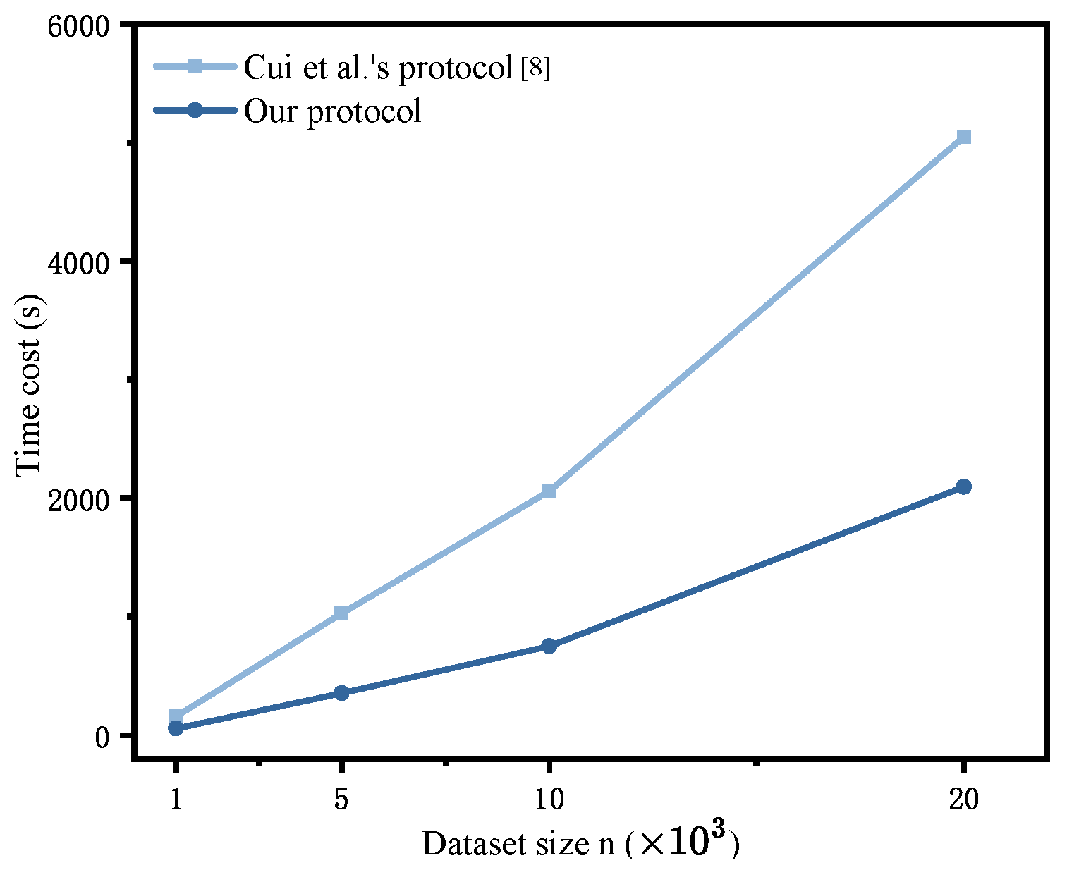
To comprehensively evaluate the practical performance of the proposed scheme, we conducted experimental comparisons of the time and communication costs between our design and Cui et al.’s protocol [8] across multiple dimensions, including but not limited to the dataset size, grid granularity m, query parameter k in kNN, and size of security parameter modulus.

All experiments were conducted on a laptop featuring an Intel^® Core^TM i5-8250U CPU (1.60 GHz, with eight logical cores, Hewlett-Packard, Palo Alto, CA, USA) with 8GB of RAM, running on Windows 10. The implementations were developed in Java using the JCA Library. Furthermore, we adopted the NIST-recommended parameters for the Digital Signature Algorithm (DSA), where the prime modulus p and subgroup order q were configured with bit lengths of 1024 and 160, respectively. Subsequently, we analyzed the impact of the following parameters:

(1)

Impact of varying n: With fixed parameters $m=16$, $k=5$, and $K=1024$, we systematically varied the dataset size n from 1000 to 20,000 to evaluate scalability. Table 7 presents the stage-wise execution times for both Cui et al.’s protocol [8] and our proposed protocol. Visually, Figure 3 further illustrates the comparative trends in the total cost of these two protocols as n increases. The results demonstrate that our protocol achieved a 58.5–65.5% reduction in time cost compared to the baseline, with the performance gap widening significantly for larger n.

(2)

Impact of varying m: Under fixed parameters $n=2000$, $k=5$, and $K=1024$, we systematically evaluated the grid granularity $m\in \{4,8,12,16,32,64\}$ to analyze algorithmic scalability. Table 8 presents a comparative analysis of computational latency (in seconds) between Cui et al.’s protocol [8] and our proposed method across these configurations. As shown in the table, the total cost of our design was about 32.7–35.4% of that of the baseline. Furthermore, as the grid granularity m primarily influences the search stages, Figure 4 visualizes the combined latencies of these phases. Notably, minimal computational overhead was achieved at $m=8$, aligning closely with the theoretical optimum derived for uniform random datasets:

$$m^2\approx \sqrt{n}\Rightarrow m\approx n^{1/4}={2000}^{1/4}\approx 6.68.$$

The empirically observed optimum ($m=8$) reflects practical implementation constraints while remaining consistent with this theoretical boundary.

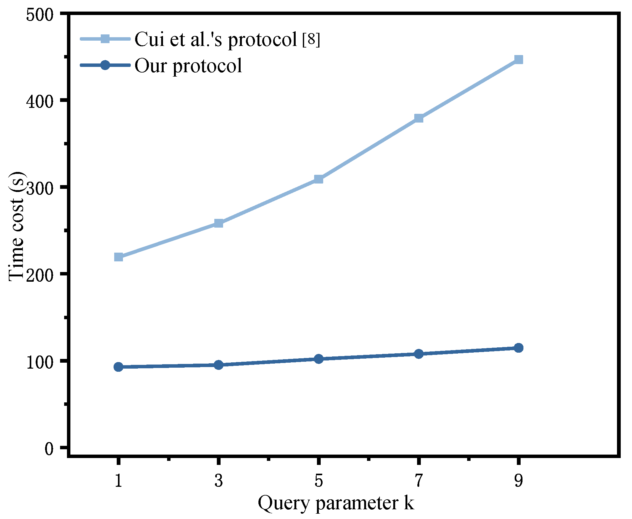
(3)

Impact of varying k: As shown in Table 9, under fixed parameters $n=2000$, $m=16$, and $K=1024$, we systematically evaluated the computational efficiency of each stage of our protocol against Cui et al.’s baseline [8] by varying the query parameter k in k-nearest-neighbor (kNN) searches from 1 to 10. Further, since the search, verification, and decryption stages are inherently dependent on k, whereas the setup, dataset encryption, and query encryption stages remain protocol-level invariants independent of k, Figure 5 illustrates the variance of the time cost of these two stages as k increases, demonstrating that the efficiency gains of our design became more pronounced as k increased.

(4)

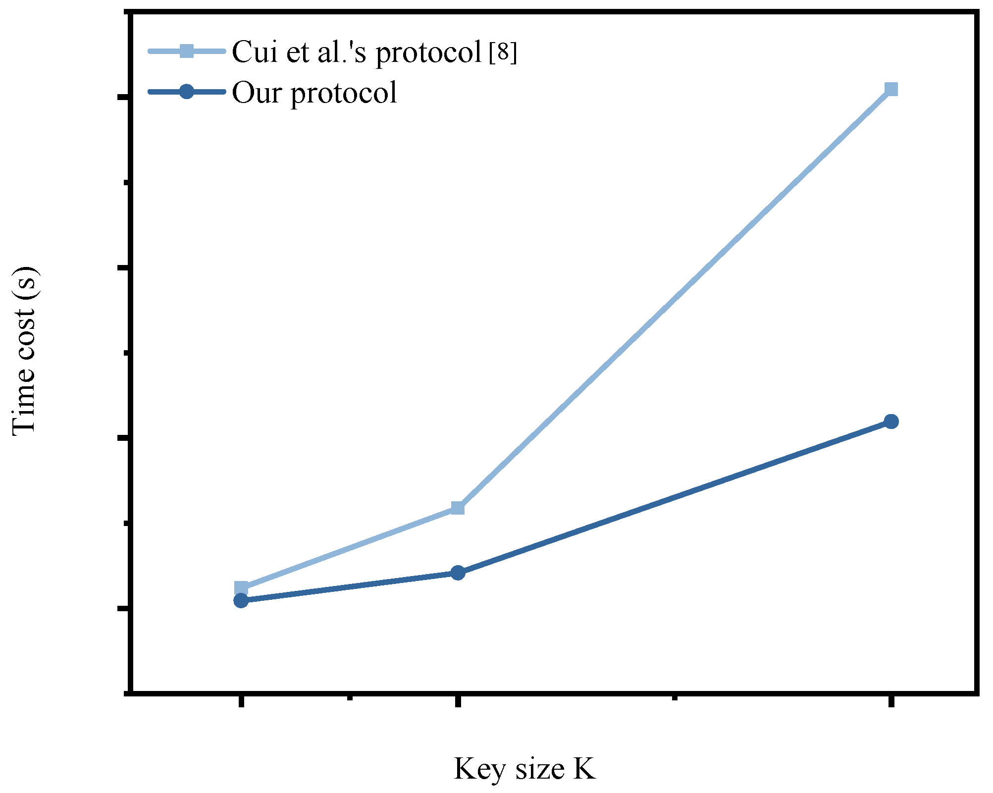
Impact of varying K: Given that the modulus size K of N determines the security strength of both the DT-PKC and Paillier cryptosystems employed in our scheme, we conducted a comprehensive performance comparison between our proposed scheme and Cui et al.’s protocol [8] under varying security levels ($K=512,1024,2048$) for fixed parameters $m=16$, $k=5$, and $n=2000$. Table 10 presents the stage-wise computational latencies (e.g., setup, encryption, search, and verification) for both schemes, explicitly quantifying the trade-off between cryptographic robustness and operational efficiency. Also, Figure 6 illustrates the total execution time scaling with increasing K, showing that the total cost of our design was about 33.8–38.1% of that of Cui et al.’s protocol.

(5)

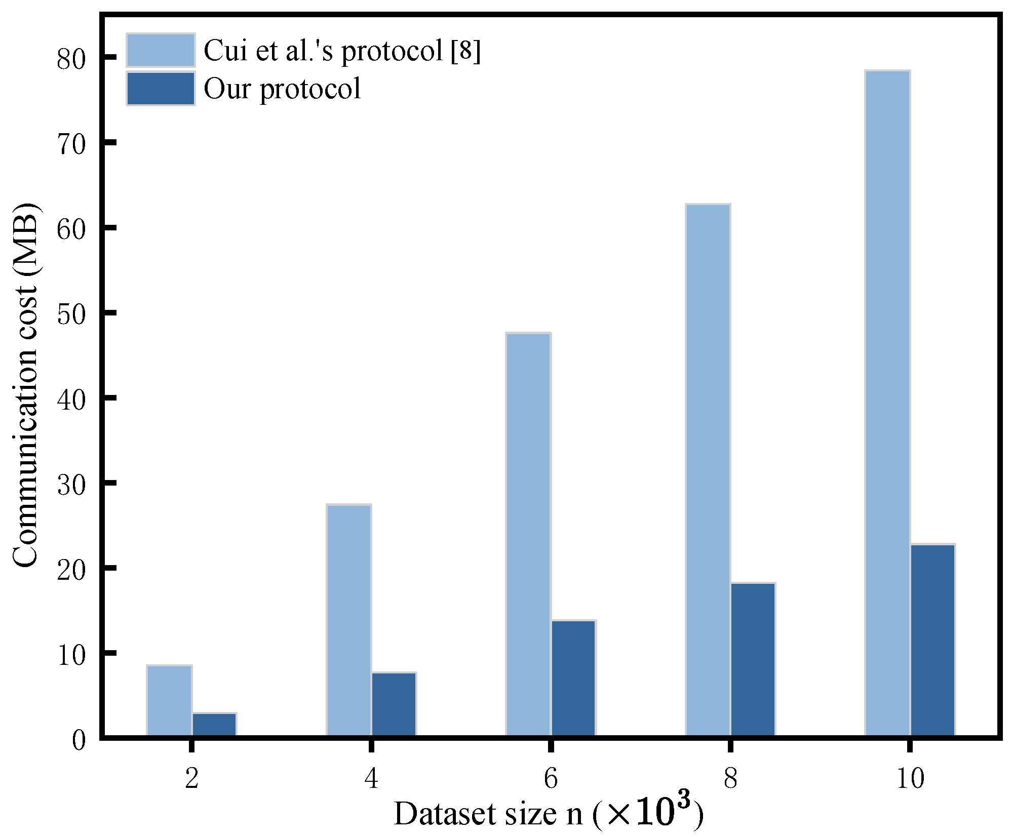
Communication cost: We conducted an experimental evaluation of communication costs with fixed parameters, $m=16$, $k=5$, and $K=1024$, while systematically varying the dataset size n. As shown in our theoretical analysis (Table 6), the primary difference in communication cost between our protocol and Cui et al.’s protocol occurred during the $\mathbf{Search}$ stage. Figure 7 illustrates the difference in communication overhead between ${\mathbf{CS}}_1$ and ${\mathbf{CS}}_2$ in our protocol compared to Cui et al.’s protocol across various dataset sizes. The polyline in Figure 8 represents the comparison of data transfer times between CS1 and CS2 during the Search phase across varying dataset sizes. The data transfer time (communication latency) was calculated as the communication volume divided by the transfer rate, with the transfer rate simulated as 390 Mbps ≈ 48.75 MB/s. Our findings demonstrated that our protocol incurred lower costs, consistent with our theoretical analysis.

Table 7. Time cost comparison on synthesized datasets with different sizes of 1000, 5000, 10,000, and 20,000 (unit: seconds).

Protocol		Cui et al.’s Protocol [8]				Our Protocol
	Dataset Size  $\mathit{n}$	1000	5000	10,000	20,000	1000	5000	10,000	20,000
Stages
$\mathbf{Setup}$		$1.448$	$1.181$	$1.211$	$1.156$	$0.312$	$0.544$	$0.279$	$0.497$
$\mathbf{DSEnc}$		$97.933$	$723.832$	$1458.838$	$3658.052$	$47.716$	$337.935$	$727.206$	$2046.939$
$\mathbf{QUEnc}$		$0.058$	$0.057$	$0.056$	$0.059$	$0.022$	$0.022$	$0.023$	$0.023$
$\mathbf{Search}$		$58.655$	$303.406$	$598.363$	$1388.696$	$8.287$	$16.914$	$24.610$	$47.330$
$\mathbf{Verify}$ and $\mathbf{ResDec}$		$0.160$	$0.534$	$0.602$	$0.722$	$0.005$	$0.005$	$0.006$	$0.008$
$\mathbf{Total}$		$158.254$	$1029.010$	$2059.070$	$5048.685$	$56.342$	$355.420$	$752.124$	$2094.797$

Figure 3. Time cost comparison for varying dataset sizes n.

Table 8. Time cost comparison with different grid granularities on a synthesized dataset of size 2000 (unit: seconds).

Protocol		Cui et al.’s Protocol [8]						Our Protocol
	Grid Granularity  $\mathit{m}$	4	8	12	16	32	64	4	8	12	16	32	64
Stages
$\mathbf{Setup}$		1.009	1.188	1.462	1.692	1.914	1.687	0.291	0.285	0.240	0.207	0.463	0.871
$\mathbf{DSEnc}$		181.751	182.137	184.899	172.719	218.232	225.192	86.298	85.202	90.337	92.901	103.423	115.173
$\mathbf{QUEnc}$		0.057	0.058	0.056	0.056	0.058	0.055	0.023	0.022	0.023	0.023	0.023	0.024
$\mathbf{Search}$		114.947	102.155	110.785	120.766	133.233	137.680	11.147	10.255	10.811	11.175	11.708	12.942
$\mathbf{Verify}$ and $\mathbf{ResDec}$		0.243	0.221	0.230	0.205	0.277	0.251	0.004	0.004	0.005	0.004	0.005	0.005
$\mathbf{Total}$		$298.007$	$285.759$	$297.432$	$309.036$	$353.714$	$364.865$	$97.763$	$95.768$	$101.456$	$104.420$	$115.622$	$129.015$

Figure 4. Time cost comparison for varying grid granularities m.

Table 9. Time cost comparison with different query parameters k on a synthesized dataset of size 2000 (unit: seconds).

Protocol		Cui et al.’s Protocol [8]					Our Protocol
	Query Parameter  $\mathit{k}$	1	3	5	7	9	1	3	5	7	9
Stages
$\mathbf{Setup}$		1.317	1.402	1.692	1.566	1.477	0.286	0.256	0.317	0.279	0.263
$\mathbf{DSEnc}$		180.479	185.852	186.317	178.708	183.617	89.623	88.044	92.901	91.075	92.367
$\mathbf{QUEnc}$		0.057	0.058	0.056	0.057	0.057	0.023	0.022	0.023	0.022	0.023
$\mathbf{Search}$		37.263	70.774	120.766	201.474	261.221	2.827	6.855	11.175	16.411	21.933
$\mathbf{Verify}$ and $\mathbf{ResDec}$		0.031	0.094	0.205	0.258	0.322	0.002	0.003	0.004	0.008	0.013
$\mathbf{Total}$		$219.147$	$258.180$	$309.036$	$382.063$	$446.694$	$92.761$	$95.180$	$104.420$	$107.795$	$114.599$

Figure 5. Time cost comparison for varying query parameters k.

Table 10. Time cost comparison with different key sizes on a synthesized dataset of size 2000 (unit: seconds).

Protocol		Cui et al.’s Protocol [8]			Our Protocol
	Key Size  $\mathit{K}$	512	1024	2048	512	1024	2048
Stages
$\mathbf{Setup}$		$0.349$	$1.192$	$6.582$	$0.192$	$0.317$	$0.535$
$\mathbf{DSEnc}$		$36.517$	$172.719$	$867.321$	$20.978$	$92.901$	$494.262$
$\mathbf{QUEnc}$		$0.009$	$0.056$	$0.267$	$0.004$	$0.023$	$0.154$
$\mathbf{Search}$		$24.160$	$120.766$	$650.312$	$2.092$	$11.175$	$53.270$
$\mathbf{Verify}$ and $\mathbf{ResDec}$		$0.055$	$0.205$	$1.067$	$0.005$	$0.004$	$0.006$
$\mathbf{Total}$		$61.090$	$309.036$	$1525.549$	$23.271$	$104.420$	$548.227$

Figure 6. Time cost comparison for varying key sizes K.

Figure 7. Communication cost comparison for ${\mathbf{CS}}_1\leftrightarrow {\mathbf{CS}}_2$ in the $\mathbf{Search}$ stage.

Figure 8. Communication latency for ${\mathbf{CS}}_1\leftrightarrow {\mathbf{CS}}_2$ in the $\mathbf{Search}$ stage.

7. Conclusions

This paper presents our investigation and proposal of a faster, privacy-preserving, and publicly verifiable protocol for exact k-nearest-neighbor queries, termed PPVkNN. Leveraging Paillier’s homomorphic encryption and a series of meticulously designed secure protocols, PPVkNN not only supports exact kNN query functionality but also preserves the privacy of data, queries, results, and query access patterns. Furthermore, it guarantees result correctness and enables public verification. Theoretical analysis confirms the correctness and security of our proposed protocols. Additionally, efficiency analysis and performance evaluation demonstrate significant computational and communication savings compared to prior works, enhancing the practicality of our scheme.

Appendix B.1. The Proof of Lemma 3

Proof. 

In Algorithm 2, due to the homomorphic property of Paillier’s cryptosystem, we know that

$$\begin{array}{cc}\hfill & x^{\prime }=E{(x_q)}^{r_1}\times E{(X/m)}^{r_1\times r_2}=E(r_1{x}_q+r_1{r}_{2}X/m),u^{\prime }=E{(X/m)}^{r_1}=E(r_{1}X/m),\hfill \\ \hfill & y^{\prime }=E{(y_q)}^{r_1}\times E{(Y/m)}^{r_1\times r_2}=E(r_1{y}_q+r_1{r}_{2}Y/m),v^{\prime }=E{(Y/m)}^{r_1}=E(r_{1}Y/m).\hfill \end{array}$$

Thus, $x=D(x^{\prime })=r_1{x}_q+r_1{r}_{2}X/m\mathrm{mod}N,$ $y=D(y^{\prime })=r_1{y}_q+r_1{r}_{2}Y/m\mathrm{mod}N,$ $u=D(u^{\prime })=r_{1}X/m\mathrm{mod}N,v=D(v^{\prime })=r_{1}Y/m\mathrm{mod}N.$ Since $r_1$ and $r_2$ are at most $\tau$ bits, and $x_q$ and $X/m$ are at most $\sigma$ bits, while N is $2\kappa$ bits, with the security parameter satisfying $\tau <\kappa -{\displaystyle \frac{\sigma +1}{2}}$, we have $x=D(x^{\prime })=r_1{x}_q+r_1{r}_{2}X/m,u=D(u^{\prime })=r_{1}X/m,y=D(y^{\prime })=r_1{y}_q+r_1{r}_{2}Y/m,v=D(v^{\prime })=r_{1}Y/m.$ Then,

$$\begin{array}{c}\hfill d_x=⌊{\displaystyle \frac{x}{u}}⌋={\displaystyle \frac{r_1{x}_q+r_1{r}_{2}X/m}{r_{1}X/m}}=⌊{\displaystyle \frac{x_q}{X/m}}⌋+r_2,d_y=⌊{\displaystyle \frac{y}{u}}⌋={\displaystyle \frac{r_1{y}_q+r_1{r}_{2}Y/m}{r_{1}Y/m}}=⌊{\displaystyle \frac{y_q}{Y/m}}⌋+r_2.\end{array}$$

Consequently, the output is

$$\begin{array}{cc}\hfill d_x^{\prime }\times E{(r_2)}^{N-1}& =E\left(⌊{\displaystyle \frac{x_q}{X/m}}⌋+r_2\right)\times E{(r_2)}^{N-1}=E\left(⌊{\displaystyle \frac{x_q}{X/m}}⌋+r_2-r_2\right)=E\left(⌊{\displaystyle \frac{x_q}{X/m}}⌋\right),\hfill \\ \hfill d_y^{\prime }\times E{(r_2)}^{N-1}& =E\left(⌊{\displaystyle \frac{y_q}{Y/m}}⌋+r_2\right)E{(r_2)}^{N-1}=E\left(⌊{\displaystyle \frac{y_q}{Y/m}}⌋+r_2-r_2\right)=E\left(⌊{\displaystyle \frac{y_q}{Y/m}}⌋\right).\hfill \end{array}$$

□

Appendix B.2. The Proof of Lemma 4

Proof. 

According to the homomorphic property of Paillier’s cryptosystem and the data-packing technique, from Step 2 of Algorithm 3, we know that

$$\begin{array}{c}\hfill {\Delta }_{xj}={\left(E\left(⌊{\displaystyle \frac{x_q}{X/m}}⌋\right)\times E{(j)}^{N-1}\times E(T)\right)}^{r_{xj}}=E\left(r_{xj}\left(⌊{\displaystyle \frac{x_q}{X/m}}⌋-j+T\right)\right),\\ \hfill {\Delta }_{yj}={\left(E\left(⌊{\displaystyle \frac{y_q}{Y/m}}⌋\right)\times E{(j)}^{N-1}\times E(T)\right)}^{r_{yj}}=E\left(r_{yj}\left(⌊{\displaystyle \frac{x_q}{X/m}}⌋-j+T\right)\right),\end{array}$$

and, in Step 9 of Algorithm 3, we have $E(G_{st}^{\prime })=E(G_{st})\times E(r_{st})=E\left(G_{st}+r_{st}\right).$ Thus, in Step 11,

$$\begin{array}{cc}\hfill {\Delta }_x^{\prime }& ={\rho }_1({\Delta }_x)=({\Delta }_{x{\rho }_1(0)},\cdots ,{\Delta }_{x{\rho }_1(m-1)})\hfill \\ \hfill & =(E(r_{x{\rho }_1(0)}(\lfloor {\displaystyle \frac{x_q}{X/m}}\rfloor -{\rho }_1(0)+T)),\cdots ,E(r_{x{\rho }_1(m-1)}(\lfloor {\displaystyle \frac{x_q}{X/m}}\rfloor -{\rho }_1(m-1)+T))),\hfill \\ \hfill {\Delta }_y^{\prime }& ={\rho }_2({\Delta }_y)=({\Delta }_{y{\rho }_2(0)},\cdots ,{\Delta }_{y{\rho }_2(m-1)})\hfill \\ \hfill & =(E(r_{y{\rho }_2(0)}(\lfloor {\displaystyle \frac{y_q}{Y/m}}\rfloor -{\rho }_2(0)+T)),\cdots ,E(r_{y{\rho }_2(m-1)}(\lfloor {\displaystyle \frac{y_q}{Y/m}}\rfloor -{\rho }_2(m-1)+T))),\hfill \\ \hfill {\Gamma }^{\prime }& ={\rho }_2({\rho }_1(E(G^{\prime })))={\left(E(G_{{\rho }_1(s){\rho }_2(t)}^{\prime })\right)}_{0\le s,t\le m-1}=(E(G_{{\rho }_1(0){\rho }_2(0)}^{\prime }),\cdots ,E(G_{{\rho }_1(m-1){\rho }_2(m-1)}^{\prime })),\hfill \end{array}$$

and, in Step 14,

$$\begin{array}{cc}\hfill v_x^{\prime }& =\prod _{i=0}^{m-1}{\Delta }_{x{\rho }_1(i)}^{2^{{\sigma }^{\prime }(m-(i+1))}}\hfill \\ & ={({\Delta }_{x{\rho }_1(0)})}^{2^{{\sigma }^{\prime }(m-1)}}\cdots ({\Delta }_{x{\rho }_1(m-1)})=E\left(\sum _{i=0}^{m-1}(r_{x{\rho }_1(i)}(\lfloor {\displaystyle \frac{x_q}{X/m}}\rfloor -{\rho }_1(i)+T))2^{{\sigma }^{\prime }(m-(i+1))}\right),\hfill \\ \hfill v_y^{\prime }& =\prod _{i=0}^{m-1}{\Delta }_{y{\rho }_2(i)}^{2^{{\sigma }^{\prime }(m-(i+1))}}\hfill \\ & ={({\Delta }_{y{\rho }_2(0)})}^{2^{{\sigma }^{\prime }(m-1)}}\cdots ({\Delta }_{y{\rho }_2(m-1)})=E\left(\sum _{i=0}^{m-1}(r_{y{\rho }_2(i)}(\lfloor {\displaystyle \frac{y_q}{Y/m}}\rfloor -{\rho }_2(i)+T))2^{{\sigma }^{\prime }(m-(i+1))}\right).\hfill \end{array}$$

Also, in Step 15, according to the property of the data-packing technique, as long as

$$\begin{array}{cc}\hfill & 0<r_{x{\rho }_1(i)}(\lfloor {\displaystyle \frac{x_q}{X/m}}\rfloor -{\rho }_1(i)+T)<2^{{\sigma }^{\prime }},\hfill \end{array}$$

(A1)

$$\begin{array}{cc}\hfill & 0<r_{y{\rho }_2(i)}(\lfloor {\displaystyle \frac{y_q}{Y/m}}\rfloor -{\rho }_2(i)+T)<2^{{\sigma }^{\prime }},\hfill \end{array}$$

(A2)

$$\begin{array}{cc}\hfill & \sum _{i=0}^{m-1}(r_{x{\rho }_1(i)}(\lfloor {\displaystyle \frac{x_q}{X/m}}\rfloor -{\rho }_1(i)+T))2^{{\sigma }^{\prime }(m-(i+1))}<N,\hfill \end{array}$$

(A3)

$$\begin{array}{cc}\hfill & \sum _{i=0}^{m-1}(r_{y{\rho }_2(i)}(\lfloor {\displaystyle \frac{y_q}{Y/m}}\rfloor -{\rho }_2(i)+T))2^{{\sigma }^{\prime }(m-(i+1))}<N,\hfill \end{array}$$

(A4)

we have

$$\begin{array}{ccc}& & \hfill (v_{x{\rho }_1(0)},\cdots ,v_{x{\rho }_1(m-1)})=D(v_x^{\prime })=((\lfloor {\displaystyle \frac{x_q}{X/m}}\rfloor -{\rho }_1(0)+T)r_{x{\rho }_1(0)},\cdots ,(\lfloor {\displaystyle \frac{x_q}{X/m}}\rfloor -{\rho }_1(m-1)+T)r_{x{\rho }_1(m-1)}),\\ & & \hfill (v_{y{\rho }_2(0)},\cdots ,v_{y{\rho }_2(m-1)})=D(v_y^{\prime })=((\lfloor {\displaystyle \frac{y_q}{Y/m}}\rfloor -{\rho }_2(0)+T)r_{y{\rho }_2(0)},\cdots ,(\lfloor {\displaystyle \frac{y_q}{Y/m}}\rfloor -{\rho }_2(m-1)+T)r_{y{\rho }_2(m-1)}).\end{array}$$

Since $r_{xj}$ and $r_{yj}(0\le j\le m-1)$ are at most $\tau$ bits, and $x_q,y_q,X/m,Y/m$ and m are at most $\sigma$ bits, with $T\ge m$ and $2^{\tau +\sigma }<2^{{\sigma }^{\prime }},2^{{\sigma }^{\prime }m}<N$, the conditions (Equations (A1)–(A4)) hold. Subsequently, in Step 18, the decisional conditions $v_{x{\rho }_1(s)}\mathrm{mod}T=0$ and $v_{y{\rho }_2(t)}\mathrm{mod}T=0$ mean that $\lfloor {\displaystyle \frac{x_q}{X/m}}\rfloor ={\rho }_1(s)$ and $\lfloor {\displaystyle \frac{y_q}{Y/m}}\rfloor ={\rho }_2(t)$. Consequently, in Step 25,

$$\begin{array}{ccc}& & \hfill E(r)=\prod _{s=0}^{m-1}\prod _{t=0}^{m-1}{(M_{st}^{\prime })}^{r_{st}}=\prod _{s=0}^{m-1}\prod _{t=0}^{m-1}{(M_{{\rho }_1^{-1}(s){\rho }_2^{-1}(t)})}^{r_{st}}=\prod _{s=0}^{m-1}\prod _{t=0}^{m-1}{(M_{st})}^{r_{{\rho }_1(s){\rho }_2(t)}}=E\left(\sum _{s=0}^{m-1}\sum _{t=0}^{m-1}{r}_{{\rho }_1(s){\rho }_2(t)}{\delta }_{st}\right)=E(r_{\widehat{s}\widehat{t}})\end{array}$$

with

$\widehat{s}=⌊{\displaystyle \frac{x_q}{X/m}}⌋,\widehat{t}=⌊{\displaystyle \frac{y_q}{Y/m}}⌋$ and

$${\delta }_{st}=\left\{\begin{array}{cc}1\hfill & ({\rho }_1(s),{\rho }_2(t))=(\widehat{s},\widehat{t})=(\lfloor {\displaystyle \frac{x_q}{X/m}}\rfloor ,\lfloor {\displaystyle \frac{y_q}{Y/m}}\rfloor )\hfill \\ 0\hfill & otherwise\hfill \end{array}\right..$$

In the last step (Step 26),

$$\begin{array}{c}\hfill {\Gamma }^{\prime }\times E{(r)}^{N-1}=E\left(G_{{\rho }_1(s){\rho }_2(t)}^{\prime }\right)\times E{(r_{\widehat{s}\widehat{t}})}^{N-1}=E\left(G_{\lfloor {\displaystyle \frac{x_q}{X/m}}\rfloor ,\lfloor {\displaystyle \frac{y_q}{Y/m}}\rfloor }+r_{\lfloor {\displaystyle \frac{x_q}{X/m}}\rfloor ,\lfloor {\displaystyle \frac{y_q}{Y/m}}\rfloor }-r_{\widehat{s}\widehat{t}}\right)=E(G_{\widehat{s}\widehat{t}}).\end{array}$$

□

Appendix B.3. The Proof of Lemma 5

Proof. 

Due to the homomorphic properties of Paillier’s cryptosystem and the data-packing technique, we know that

$$\begin{array}{cc}\hfill v_0^{\prime }=& {(E(G_{st})\times E({\Phi }_0))}^{r_0}=(E(i_1^{(st)}|x_{i_1^{(st)}}|y_{i_1}^{(st)}|\cdots |i_{\lambda }^{(st)}|x_{i_{\lambda }^{(st)}}|y_{i_{\lambda }^{(st)}}{)\times E\left(r_1|r_2|\cdots |r_{3\lambda }\right))}^{r_0}\hfill \\ \hfill =& E(r_0(i_1^{(st)}+r_1)2^{{\sigma }^{\prime }(3\lambda -1)}+r_0(x_{i_1^{(st)}}+r_2)2^{{\sigma }^{\prime }(3\lambda -2)}+r_0(y_{i_1^{(st)}}+r_3)2^{{\sigma }^{\prime }(3\lambda -3)}+\cdots +r_0(y_{i_{\lambda }^{(st)}}+r_{3\lambda })2^0),\hfill \\ \hfill v_1^{\prime }=& {(E(Q^{\prime })\times E({\Phi }_1))}^{r_0}={(E\left(x_q|y_q|\cdots |x_q|y_q|\cdots |x_q|y_q\right)\times E\left(r_2|r_3|\cdots |r_{3k-1}|r_{3k}|\cdots |r_{3\lambda -1}|r_{3\lambda }\right))}^{r_0}\hfill \\ \hfill =& E(r_0(x_q+r_2)2^{{\sigma }^{\prime }(2\lambda -1)}+r_0(y_q+r_3)2^{{\sigma }^{\prime }(2\lambda -2)}+\cdots +r_0(y_q+r_{3\lambda })2^0),\hfill \\ \hfill v_2^{\prime }=& {(E(i{d}^{\prime })\times E({\Phi }_2))}^{r_0}=(E\left(id|id|id|\cdots |id\right)\times E(r_1|r_4|r_7|\cdots |r_{3\lambda -2}{))}^{r_0}\hfill \\ \hfill =& E(r_0(id+r_1)2^{{\sigma }^{\prime }(\lambda -1)}+r_0(id+r_4)2^{{\sigma }^{\prime }(\lambda -2)}+r_0(id+r_7)2^{{\sigma }^{\prime }(\lambda -3)}+\cdots +r_0(id+r_{3\lambda -2})2^0).\hfill \end{array}$$

Thus,

$$\begin{array}{cc}\hfill v_0& =D(v_0)=r_0(i_1^{(st)}+r_1)2^{{\sigma }^{\prime }(3\lambda -1)}+r_0(x_{i_1^{(st)}}+r_2)2^{{\sigma }^{\prime }(3\lambda -2)}+r_0(y_{i_1^{(st)}}+r_3)2^{{\sigma }^{\prime }(3\lambda -3)}+\cdots +r_0(y_{i_{\lambda }^{(st)}}+r_{3\lambda })2^0\mathrm{mod}N,\hfill \\ \hfill v_1& =D(v_1)=r_0(x_q+r_2)2^{{\sigma }^{\prime }(2\lambda -1)}+r_0(y_q+r_3)2^{{\sigma }^{\prime }(2\lambda -2)}+\cdots +r_0(y_q+r_{3\lambda })2^0\mathrm{mod}N,\hfill \\ \hfill v_2& =D(v_2)=r_0(id+r_1)2^{{\sigma }^{\prime }(\lambda -1)}+r_0(id+r_4)2^{{\sigma }^{\prime }(\lambda -2)}+r_0(id+r_7)2^{{\sigma }^{\prime }(\lambda -3)}+\cdots +r_0(id+r_{3\lambda -2})2^0\mathrm{mod}N.\hfill \end{array}$$

Since $r_j(0\le j\le 3\lambda )$ are at most $\tau$ bits, $i_j^{(st)},x_{i_j^{(st)}},y_{i_j^{(st)}}(1\le j\le \lambda ),x_q$, $y_q$ and $id$ are at most $\sigma$ bits, and the security parameters $\tau$ and ${\sigma }^{\prime }$ satisfy $2^{\tau +\sigma }<2^{{\sigma }^{\prime }}$ and $2^{{\sigma }^{\prime }3\lambda }<N$, we have

$$\begin{array}{cc}\hfill & v_0=D(v_0)=r_0(i_1^{(st)}+r_1)2^{{\sigma }^{\prime }(3\lambda -1)}+r_0(x_{i_1^{(st)}}+r_2)2^{{\sigma }^{\prime }(3\lambda -2)}+r_0(y_{i_1^{(st)}}+r_3)2^{{\sigma }^{\prime }(3\lambda -3)}+\cdots +r_0(y_{i_{\lambda }^{(st)}}+r_{3\lambda })2^0,\hfill \\ \hfill & v_1=D(v_1)=r_0(x_q+r_2)2^{{\sigma }^{\prime }(2\lambda -1)}+r_0(y_q+r_3)2^{{\sigma }^{\prime }(2\lambda -2)}+\cdots +r_0(y_q+r_{3\lambda })2^0,\hfill \\ \hfill & v_2=D(v_2)=r_0(id+r_1)2^{{\sigma }^{\prime }(\lambda -1)}+r_0(id+r_4)2^{{\sigma }^{\prime }(\lambda -2)}+r_0(id+r_7)2^{{\sigma }^{\prime }(\lambda -3)}+\cdots +r_0(id+r_{3\lambda -2})2^0,\hfill \\ \hfill & \mathbf{ID}=\{r_0(i_1^{(st)}+r_1),r_0(i_2^{(st)}+r_4),r_0(i_3^{(st)}+r_7),\cdots ,r_0(i_{\lambda }^{(st)}+r_{3\lambda -2})\}\hfill \\ \hfill & \mathbf{P}=\left\{(r_0(x_{i_1^{(st)}}+r_2),r_0(y_{i_1^{(st)}}+r_3)),(r_0(x_{i_2^{(st)}}+r_5),r_0(y_{i_2^{(st)}}+r_6)),\cdots ,(r_0(x_{i_{\lambda }^{(st)}}+r_{3\lambda -1}),r_0(y_{i_{\lambda }^{(st)}}+r_{3\lambda }))\right\}\hfill \\ \hfill & \mathbf{Q}=\{\left(r_0(x_q+r_2),r_0(y_q+r_3)\right),\left(r_0(x_q+r_5),r_0(y_q+r_6)\right),\cdots ,\left(r_0(x_q+r_{3\lambda -1}),r_0(y_q+r_{3\lambda })\right)\}\hfill \\ \hfill & \mathbf{id}=\{r_0(id+r_1),r_0(id+r_4),r_0(id+r_7),\cdots ,r_0(id+r_{3\lambda -2})\}\hfill \end{array}$$

Subsequently, after the for-loop in Step 20, we have

$$\begin{array}{cccc}& & \hfill d_{\min }& =\underset{0\le j\le \lambda -1,i_{j+1}^{(st)}\ne id}{\min }{r}_0^2\left({(x_{i_{j+1}^{(st)}}-x_q)}^2+{(y_{i_{j+1}^{(st)}}-y_q)}^2\right)=r_0^2\left({(x_{i_{pos+1}^{(st)}}-x_q)}^2+{(y_{i_{pos+1}^{(st)}}-y_q)}^2\right),\hfill \end{array}$$

and, in Step 28,

$$\begin{array}{cc}\hfill & E(r_{id})=\prod _{i=0}^{\lambda -1}\delta {\left[i\right]}^{r_{3i+1}}=\delta {\left[0\right]}^{r_1}\delta {\left[1\right]}^{r_4}\delta {\left[2\right]}^{r_7}\cdots \delta {[\lambda -1]}^{r_{3\lambda -2}}=E(r_1·0+\cdots +r_{3pos+1}·1+\cdots +r_{3\lambda -2}·0)=E(r_{3pos+1}),\hfill \\ \hfill & E(r_x)=\prod _{i=0}^{\lambda -1}\delta {\left[i\right]}^{r_{3i+2}}=\delta {\left[0\right]}^{r_2}\delta {\left[1\right]}^{r_5}\delta {\left[2\right]}^{r_8}\cdots \delta {[\lambda -1]}^{r_{3\lambda -1}}=E(r_2·0+\cdots +r_{3pos+2}·1+\cdots +r_{3\lambda -1}·0)=E(r_{3pos+2}),\hfill \\ \hfill & E(r_y)=\prod _{i=0}^{\lambda -1}\delta {\left[i\right]}^{r_{3i+3}}=\delta {\left[0\right]}^{r_3}\delta {\left[1\right]}^{r_6}\delta {\left[2\right]}^{r_9}\cdots \delta {[\lambda -1]}^{r_{3\lambda }}=E(r_3·0+\cdots +r_{3pos+3}·1+\cdots +r_{3\lambda }·0)=E(r_{3pos+3}).\hfill \end{array}$$

Therefore, in the last step (Step 29), by the homomorphic property,

$$\begin{array}{cc}\hfill E(i{d}_{min})& =E{(\mathbf{ID}\left[pos\right])}^{r_0^{-1}}\times E{(r_{id})}^{N-1}=E(r_0^{-1}\mathbf{ID}\left[pos\right]-r_{id})=E(r_0^{-1}(r_0(i_{pos+1}^{(st)}+r_{3pos+1}))-r_{3pos+1})=E\left(i_{pos+1}^{(st)}\right),\hfill \\ \hfill E(x_{i{d}_{min}})& =E{(\mathbf{P}\left[pos\right].x)}^{r_0^{-1}}\times E{(r_x)}^{N-1}=E(r_0^{-1}\mathbf{P}\left[pos\right].x-r_x)=E(r_0^{-1}(r_0(x_{i_{pos+1}^{(st)}}+r_{3pos+2}))-r_{3pos+2})=E\left(x_{i_{pos+1}^{(st)}}\right),\hfill \\ \hfill E(y_{i{d}_{min}})& =E{(\mathbf{P}\left[pos\right].y)}^{r_0^{-1}}\times E{(r_y)}^{N-1}=E(r_0^{-1}\mathbf{P}\left[pos\right].y-r_y)=E(r_0^{-1}(r_0(y_{i_{pos+1}^{(st)}}+r_{3pos+3}))-r_{3pos+3})=E\left(y_{i_{pos+1}^{(st)}}\right).\hfill \end{array}$$

□

Appendix B.4. The Proof of Lemma 6

Proof. 

According to the homomorphic property, in Step 3, we know that for $0\le j\le \lceil {\displaystyle \frac{n}{w}}\rceil -1$,

$$\begin{array}{cc}\hfill & E({\eta }_{Mj})={(E((j+1)w-1)\times E(r_{0j}))}^{r_{1j}}=E(r_{1j}((j+1)w-1+r_{0j})),\hfill \\ \hfill & E({\eta }_j)={(E(i{d}_{\min })\times E(r_{0j}))}^{r_{1j}}=E(r_{1j}(i{d}_{\min }+r_{0j})),\hfill \\ \hfill & E({\eta }_{mj})={(E(jw)\times E(r_{0j}))}^{r_{1j}}=E(r_{1j}(jw+r_{0j})),\hfill \end{array}$$

and, in Step 7, for $0\le j\le \lceil {\displaystyle \frac{n}{w}}\rceil -1$ and $0\le k\le w-1$, we have

$$\begin{array}{cc}\hfill & {\Psi }_{(jw+k)0}={(E(jw+k)\times E{(i{d}_{\min })}^{N-1})}^{r_{(jw+k)0}}=E(r_{(jw+k)0}(jw+k-i{d}_{\min })),\hfill \\ \hfill & {\Psi }_{(jw+k)1}=E(VRV(P_{jw+k}))\times E(r_{(jw+k)1})=E(VRV(P_{jw+k})+r_{(jw+k)1}),\hfill \\ \hfill & {\Psi }_{(jw+k)2}=E(Sig(P_{jw+k}))\times E(r_{(jw+k)2})=E(Sig(P_{jw+k})+r_{(jw+k)2}).\hfill \end{array}$$

Thus, in Step 13,

$$\begin{array}{cc}\hfill & {\eta }_M^{\prime \prime }={\rho }_1({\eta }_M^{\prime })=(E({\eta }_{M{\rho }_1(0)}),\cdots ,E({\eta }_{M{\rho }_1(\lceil {\displaystyle \frac{n}{w}}\rceil -1)})),{\eta }_m^{\prime \prime }={\rho }_1({\eta }_m^{\prime })=(E({\eta }_{m{\rho }_1(0)}),\cdots ,E({\eta }_{m{\rho }_1(\lceil {\displaystyle \frac{n}{w}}\rceil -1)})),\hfill \\ \hfill & {\eta }^{\prime \prime }={\rho }_1({\eta }^{\prime })=(E({\eta }_{{\rho }_1(0)}),\cdots ,E({\eta }_{{\rho }_1(\lceil {\displaystyle \frac{n}{w}}\rceil -1)})),{\mathcal{B}}^{\prime \prime }={\rho }_2({\rho }_1({\mathcal{B}}^{\prime }))=\left({\Psi }_0^{\prime },{\Psi }_1^{\prime },{\Psi }_2^{\prime }\right),\hfill \\ \hfill & \left({\Psi }_0^{\prime },{\Psi }_1^{\prime },{\Psi }_2^{\prime }\right)=\left(\left({\Psi }_{{\rho }_1(0)0}^{\prime },\cdots ,{\Psi }_{{\rho }_1\left(\lceil {\displaystyle \frac{n}{w}}\rceil -1\right),0}^{\prime }\right),\left({\Psi }_{{\rho }_1(0)1}^{\prime },\cdots ,{\Psi }_{{\rho }_1\left(\lceil {\displaystyle \frac{n}{w}}\rceil -1\right),1}^{\prime }\right),\left({\Psi }_{{\rho }_1(0)2}^{\prime },\cdots ,{\Psi }_{{\rho }_1\left(\lceil {\displaystyle \frac{n}{w}}\rceil -1\right),2}^{\prime }\right)\right)=\hfill \\ \hfill & \left({\left({\Psi }_{({\rho }_1(j)w+{\rho }_2(k))0}\right)}_{0\le j\le (\lceil {\displaystyle \frac{n}{w}}\rceil -1),0\le k\le w-1},{\left({\Psi }_{({\rho }_1(j)w+{\rho }_2(k))1}\right)}_{0\le j\le (\lceil {\displaystyle \frac{n}{w}}\rceil -1),0\le k\le w-1},{\left({\Psi }_{({\rho }_1(j)w+{\rho }_2(k))2}\right)}_{0\le j\le (\lceil {\displaystyle \frac{n}{w}}\rceil -1),0\le k\le w-1}\right),\hfill \end{array}$$

which results in the following in Step 19:

$$\begin{array}{ccc}& & \hfill ({\eta }_{M{\rho }_1(0)},\cdots ,{\eta }_{M{\rho }_1(\lceil {\displaystyle \frac{n}{w}}\rceil -1)})=D({\eta }_M^{\prime \prime }),({\eta }_{m{\rho }_1(0)},\cdots ,{\eta }_{m{\rho }_1(\lceil {\displaystyle \frac{n}{w}}\rceil -1)})=D({\eta }_m^{\prime \prime }),({\eta }_{{\rho }_1(0)},\cdots ,{\eta }_{{\rho }_1(\lceil {\displaystyle \frac{n}{w}}\rceil -1)})=D({\eta }^{\prime \prime }).\end{array}$$

Consequently, in Step 22, the condition $({\eta }_{M{\rho }_1(j)}-{\eta }_{{\rho }_1(j)})\ge 0\wedge ({\eta }_{m{\rho }_1(j)}-{\eta }_{{\rho }_1(j)})<0$ is equivalent to

$$\begin{array}{cc}\hfill & (r_{1{\rho }_1(j)}(({\rho }_1(j)+1)w-1+r_{0{\rho }_1(j)}))\mathrm{mod}N-(r_{1{\rho }_1(j)}(i{d}_{\min }+r_{0{\rho }_1(j)}))\mathrm{mod}N\ge 0,\hfill \end{array}$$

(A5)

$$\begin{array}{cc}\hfill & (r_{1{\rho }_1(j)}(({\rho }_1(j))w+r_{0{\rho }_1(j)}))\mathrm{mod}N-(r_{1{\rho }_1(j)}(i{d}_{\min }+r_{0{\rho }_1(j)}))\mathrm{mod}N<0.\hfill \end{array}$$

(A6)

Since $r_{0j}$ and $r_{1j}>0$ are at most $\tau$ bits, $i{d}_{\min }$ and $(\lceil {\displaystyle \frac{n}{w}}\rceil )w-1<n$ are at most $\sigma$ bits, and the security parameter $\tau$ satisfies $2^{\tau +\sigma }<N$ and $2^{2\tau }<N$, Equations (A5) and (A6) are

$$\begin{array}{cc}\hfill & r_{1{\rho }_1(j)}(({\rho }_1(j)+1)w-1+r_{0{\rho }_1(j)})-r_{1{\rho }_1(j)}(i{d}_{\min }+r_{0{\rho }_1(j)})\ge 0\iff ({\rho }_1(j)+1)w-1\ge i{d}_{\min },\hfill \end{array}$$

(A7)

$$\begin{array}{cc}\hfill & r_{1{\rho }_1(j)}(({\rho }_1(j))w+r_{0{\rho }_1(j)})-r_{1{\rho }_1(j)}(i{d}_{\min }+r_{0{\rho }_1(j)})<0\iff {\rho }_1(j)w<i{d}_{\min },\hfill \end{array}$$

(A8)

which means that $i{d}_{\min }$ lies in the bucket ${\mathcal{B}}_{{\rho }_1(j)}$. Then, Step 23 decrypts the entry in each row of this bucket:

$$\begin{array}{c}\hfill ({\psi }_{({\rho }_1(j)w+{\rho }_2(0))0},\cdots ,{\psi }_{({\rho }_1(j)w+{\rho }_2(w-1))0})=D({\Psi }_{{\rho }_1(j)0}^{\prime }).\end{array}$$

Thus, the condition in Step 25 is ${\psi }_{({\rho }_1(j)w+{\rho }_2(k))0}=r_{({\rho }_1(j)w+{\rho }_2(k))0}({\rho }_1(j)w+{\rho }_2(k)-i{d}_{\min })=0,$ which means that $i{d}_{\min }={\rho }_1(j)w+{\rho }_2(k)$. At this point, we record the ciphertexts of the $VRV(P_{i{d}_{\min }})$ and the signature in Step 26:

$$\begin{array}{ccc}& & \hfill \Theta =\left({\Psi }_{({\rho }_1(j)w+{\rho }_2(k))1},{\Psi }_{({\rho }_1(j)w+{\rho }_2(k))2}\right)=\left({\Psi }_{(i{d}_{\min })1},{\Psi }_{(i{d}_{\min })2}\right)=\left(E(VRV(P_{i{d}_{\min }})+r_{i{d}_{\min }1}),E(Sig(P_{i{d}_{\min }})+r_{i{d}_{\min }1}))\right).\end{array}$$

Consequently, in Step 30,

$$\begin{array}{cc}\hfill E({\psi }^{(1)})& =\prod _{j=0}^{\lceil {\displaystyle \frac{n}{w}}\rceil -1}\prod _{k=0}^{w-1}{(M_{jk}^{\prime })}^{r_{(jw+k)1}}=\prod _{j=0}^{\lceil {\displaystyle \frac{n}{w}}\rceil -1}\prod _{k=0}^{w-1}{(M_{{\rho }_1^{-1}(j){\rho }_2^{-1}(k)})}^{r_{(jw+k)1}}=\prod _{j=0}^{\lceil {\displaystyle \frac{n}{w}}\rceil -1}\prod _{k=0}^{w-1}{(M_{jk})}^{r_{({\rho }_1(j)w+{\rho }_2(k))1}}\hfill \\ & =E\left(\sum _{j=0}^{\lceil {\displaystyle \frac{n}{w}}\rceil -1}\sum _{k=0}^{w-1}{\delta }_{jk}{r}_{({\rho }_1(j)w+{\rho }_2(k))1}\right)=E(r_{i{d}_{\min }1}),\hfill \end{array}$$

$$\begin{array}{cc}\hfill E({\psi }^{(2)})& =\prod _{j=0}^{\lceil {\displaystyle \frac{n}{w}}\rceil -1}\prod _{k=0}^{w-1}{(M_{jk}^{\prime })}^{r_{(jw+k)2}}=\prod _{j=0}^{\lceil {\displaystyle \frac{n}{w}}\rceil -1}\prod _{k=0}^{w-1}{(M_{{\rho }_1^{-1}(j){\rho }_2^{-1}(k)})}^{r_{(jw+k)2}}=\prod _{j=0}^{\lceil {\displaystyle \frac{n}{w}}\rceil -1}\prod _{k=0}^{w-1}{(M_{jk})}^{r_{({\rho }_1(j)w+{\rho }_2(k))2}}\hfill \\ \hfill & =E\left(\sum _{j=0}^{\lceil {\displaystyle \frac{n}{w}}\rceil -1}\sum _{k=0}^{w-1}{\delta }_{jk}{r}_{({\rho }_1(j)w+{\rho }_2(k))2}\right)=E(r_{i{d}_{\min }2})\hfill \end{array}$$

with ${\delta }_{jk}=\left\{\begin{array}{cc}1\hfill & {\rho }_1(j)w+{\rho }_2(k)=i{d}_{\min }\hfill \\ 0\hfill & otherwise\hfill \end{array}\right.,$ and, in the last step (Step 31),

$$\begin{array}{cc}\hfill & {\Theta }_1\times E{({\psi }^{(1)})}^{N-1}=E(VRV(P_{i{d}_{\min }})+r_{i{d}_{\min }1})\times E{(r_{i{d}_{\min }1})}^{N-1}=E(VRV(P_{i{d}_{\min }})),\hfill \\ \hfill & {\Theta }_2\times E{({\psi }^{(2)})}^{N-1}=E(Sig(P_{i{d}_{\min }})+r_{i{d}_{\min }2})\times E{(r_{i{d}_{\min }2})}^{N-1}=E(Sig(P_{i{d}_{\min }})).\hfill \end{array}$$

□

Appendix B.5. The Proof of Lemma 7

Proof. 

Given the correctness established by Lemmas 3–5 for Algorithms 2–4, it follows that in Step 4, the two-tuple $(E(x_{i{d}_{min}^{(1)}}),E(y_{i{d}_{min}^{(1)}}))$ represents the encrypted nearest-neighbor point to Q. Due to the homomorphic property of Paillier’s cryptosystem, after Steps 5–7, $(x_{i{d}_{\min }^{(1)}}^{\prime },y_{i{d}_{\min }^{(1)}}^{\prime })=(x_{i{d}_{\min }^{(1)}}+r_2^{(1)},y_{i{d}_{\min }^{(1)}}+r_3^{(1)})$, and $P_{i{d}_{\min }^{(1)}}=(x_{i{d}_{\min }^{(1)}},y_{i{d}_{\min }^{(1)}})$ is the nearest neighbor to Q. Also, by Lemma 6 and the homomorphic property, after Steps 8–11, we have $Sig{(P_{i{d}_{\min }^{(1)}})}^{\prime }=Sig(P_{i{d}_{\min }^{(1)}})+r_5^{(1)}$ and

$$\begin{array}{cccc}& & \hfill VRV{(P_{i{d}_{\min }^{(1)}})}^{\prime }& =(i{d}_1^{(1)}+r_{4,1}^{(1)})2^{\sigma (3L-1)}+(x_{i{d}_1^{(1)}}+r_{4,2}^{(1)})2^{\sigma (3L-2)}+(y_{i{d}_1^{(1)}}+r_{4,3}^{(1)})2^{\sigma (3L-3)}+\cdots +(y_{i{d}_L^{(1)}}+r_{4,3L}^{(1)})2^0.\hfill \end{array}$$

Thus, after the unpacking operation in Step 12,

$$\begin{array}{ccc}& & \hfill \left\{{i{d}_1^{(1)}}^{\prime },P_{{i{d}_1^{(1)}}^{\prime }}^{\prime },\cdots ,{i{d}_L^{(1)}}^{\prime },P_{{i{d}_L^{(1)}}^{\prime }}^{\prime }\right\}=\left\{i{d}_1^{(1)}+r_{4,1}^{(1)},P_{i{d}_1^{(1)}}+\right.\left.(r_{4,2}^{(1)},r_{4,3}^{(1)}),\cdots ,i{d}_L^{(1)}+r_{4,3L-2}^{(1)},P_{i{d}_L^{(1)}}+(r_{4,3L-1}^{(1)},r_{4,3L}^{(1)})\right\}.\end{array}$$

Through a similar analysis, we can also prove the cases for $j=2,\cdots ,k$. □

References

1. Wang, J.; Chen, X. Efficient and Secure Storage for Outsourced Data: A Survey; Springer: Berlin/Heidelberg, Germany, 2016; Volume 1, pp. 178–188. [Google Scholar] [CrossRef]
2. Lei, X.; Liu, A.X.; Li, R.; Tu, G.H. SecEQP: A Secure and Efficient Scheme for SkNN Query Problem Over Encrypted Geodata on Cloud. In Proceedings of the 2019 IEEE 35th International Conference on Data Engineering (ICDE), Macao, China, 8–11 April 2019; pp. 662–673. [Google Scholar] [CrossRef]
3. Liu, Q.; Hao, Z.; Peng, Y.; Jiang, H.; Wu, J.; Peng, T.; Wang, G.; Zhang, S. SecVKQ: Secure and verifiable kNN queries in sensor–cloud systems. J. Syst. Archit. 2021, 120, 102300. [Google Scholar] [CrossRef]
4. Zhang, Y.; Wang, B.; Zhao, Z. Secure k-NN Query With Multiple Keys Based on Random Projection Forests. IEEE Internet Things J. 2024, 11, 15205–15218. [Google Scholar] [CrossRef]
5. Qi, J.; Jia, X.; Luo, M.; Feng, Q. A Privacy-Aware K-Nearest Neighbor Query Scheme for Location-Based Services. IEEE Internet Things J. 2024, 11, 10831–10842. [Google Scholar] [CrossRef]
6. Cheng, K.; Wang, L.; Shen, Y.; Wang, H.; Wang, Y.; Jiang, X.; Zhong, H. Secure k-NN Query on Encrypted Cloud Data with Multiple Keys. IEEE Trans. Big Data 2021, 7, 689–702. [Google Scholar] [CrossRef]
7. Sundarapandi, G.P.; Bokhary, S.; Samanthula, B.K.; Dong, B. A Probabilistic Approach for Secure and Verifiable Computation of kNN Queries in Cloud. In Proceedings of the 2023 IEEE Cloud Summit, Baltimore, MD, USA, 6–7 July 2023; pp. 15–20. [Google Scholar] [CrossRef]
8. Cui, N.; Qian, K.; Cai, T.; Li, J.; Yang, X.; Cui, J.; Zhong, H. Towards Multi-User, Secure, and Verifiable kNN Query in Cloud Database. IEEE Trans. Knowl. Data Eng. 2023, 35, 9333–9349. [Google Scholar] [CrossRef]
9. Cui, N.; Yang, X.; Wang, B.; Li, J.; Wang, G. SVkNN: Efficient Secure and Verifiable k-Nearest Neighbor Query on the Cloud Platform. In Proceedings of the 2020 IEEE 36th International Conference on Data Engineering (ICDE), Dallas, TX, USA, 20–24 April 2020; pp. 253–264. [Google Scholar] [CrossRef]
10. Oliveira, S.R.; Zaiane, O.R. Privacy preserving clustering by data transformation. J. Inf. Data Manag. 2010, 1, 37. [Google Scholar]
11. Wong, W.K.; Cheung, D.W.l.; Kao, B.; Mamoulis, N. Secure kNN computation on encrypted databases. In Proceedings of the 2009 ACM SIGMOD International Conference on Management of Data, New York, NY, USA, 29 June–2 July 2009; SIGMOD ’09. pp. 139–152. [Google Scholar] [CrossRef]
12. Hu, H.; Xu, J.; Ren, C.; Choi, B. Processing private queries over untrusted data cloud through privacy homomorphism. In Proceedings of the 2011 IEEE 27th International Conference on Data Engineering, Hannover, Germany, 11–16 April 2011; pp. 601–612. [Google Scholar] [CrossRef]
13. Yao, B.; Li, F.; Xiao, X. Secure nearest neighbor revisited. In Proceedings of the 2013 IEEE 29th International Conference on Data Engineering (ICDE), Brisbane, QLD, Australia, 8–12 April 2013; pp. 733–744. [Google Scholar] [CrossRef]
14. Choi, S.; Ghinita, G.; Lim, H.S.; Bertino, E. Secure kNN Query Processing in Untrusted Cloud Environments. IEEE Trans. Knowl. Data Eng. 2014, 26, 2818–2831. [Google Scholar] [CrossRef]
15. Wang, B.; Hou, Y.; Li, M. QuickN: Practical and Secure Nearest Neighbor Search on Encrypted Large-Scale Data. IEEE Trans. Cloud Comput. 2022, 10, 2066–2078. [Google Scholar] [CrossRef]
16. Popa, R.A.; Li, F.H.; Zeldovich, N. An Ideal-Security Protocol for Order-Preserving Encoding. In Proceedings of the 2013 IEEE Symposium on Security and Privacy, Berkeley, CA, USA, 19–22 May 2013; pp. 463–477. [Google Scholar] [CrossRef]
17. Zhu, Y.; Xu, R.; Takagi, T. Secure k-NN computation on encrypted cloud data without sharing key with query users. In Proceedings of the 2013 International Workshop on Security in Cloud Computing, Hangzhou, China, 8 May 2013; Cloud Computing ’13. pp. 55–60. [Google Scholar] [CrossRef]
18. Zhu, Y.; Huang, Z.; Takagi, T. Secure and controllable k-NN query over encrypted cloud data with key confidentiality. J. Parallel Distrib. Comput. 2016, 89, 1–12. [Google Scholar] [CrossRef]
19. Lei, X.; Tu, G.H.; Liu, A.X.; Xie, T. Fast and Secure kNN Query Processing in Cloud Computing. In Proceedings of the 2020 IEEE Conference on Communications and Network Security (CNS), Avignon, France, 29 June–1 July 2020; pp. 1–9. [Google Scholar] [CrossRef]
20. Li, R.; Liu, A.X.; Xu, H.; Liu, Y.; Yuan, H. Adaptive Secure Nearest Neighbor Query Processing Over Encrypted Data. IEEE Trans. Dependable Secur. Comput. 2022, 19, 91–106. [Google Scholar] [CrossRef]
21. Zheng, Y.; Lu, R.; Zhang, S.; Shao, J.; Zhu, H. Achieving Practical and Privacy-Preserving kNN Query over Encrypted Data. In IEEE Transactions on Dependable and Secure Computing; IEEE: Piscataway, NJ, USA, 2024; pp. 1–13. [Google Scholar] [CrossRef]
22. Elmehdwi, Y.; Samanthula, B.K.; Jiang, W. Secure k-nearest neighbor query over encrypted data in outsourced environments. In Proceedings of the 2014 IEEE 30th International Conference on Data Engineering, Chicago, IL, USA, 31 March–4 April 2014; pp. 664–675. [Google Scholar] [CrossRef]
23. Guan, Y.; Lu, R.; Zheng, Y.; Shao, J.; Wei, G. Toward Oblivious Location-Based k-Nearest Neighbor Query in Smart Cities. IEEE Internet Things J. 2021, 8, 14219–14231. [Google Scholar] [CrossRef]
24. Yiu, M.L.; Lo, E.; Yung, D. Authentication of moving kNN queries. In Proceedings of the 2011 IEEE 27th International Conference on Data Engineering, Hannover, Germany, 11–16 April 2011; pp. 565–576. [Google Scholar] [CrossRef]
25. Rong, H.; Wang, H.; Liu, J.; Wu, W.; Xian, M. Efficient Integrity Verification of Secure Outsourced kNN Computation in Cloud Environments. In Proceedings of the 2016 IEEE Trustcom/BigDataSE/ISPA, Tianjin, China, 23–26 August 2016; pp. 236–243. [Google Scholar] [CrossRef]
26. Jiang, S.; Zhu, X.; Guo, L.; Liu, J. Publicly Verifiable Boolean Query Over Outsourced Encrypted Data. IEEE Trans. Cloud Comput. 2019, 7, 799–813. [Google Scholar] [CrossRef]
27. Wu, S.; Li, Q.; Li, G.; Yuan, D.; Yuan, X.; Wang, C. ServeDB: Secure, Verifiable, and Efficient Range Queries on Outsourced Database. In Proceedings of the 2019 IEEE 35th International Conference on Data Engineering (ICDE), Macao, China, 8–11 April 2019; pp. 626–637. [Google Scholar] [CrossRef]
28. Liu, X.; Deng, R.H.; Choo, K.K.R.; Weng, J. An Efficient Privacy-Preserving Outsourced Calculation Toolkit With Multiple Keys. IEEE Trans. Inf. Forensics Secur. 2016, 11, 2401–2414. [Google Scholar] [CrossRef]
29. Yi, X.; Paulet, R.; Bertino, E.; Varadharajan, V. Practical Approximate k Nearest Neighbor Queries with Location and Query Privacy. IEEE Trans. Knowl. Data Eng. 2016, 28, 1546–1559. [Google Scholar] [CrossRef]
30. Benabbas, S.; Gennaro, R.; Vahlis, Y. Verifiable Delegation of Computation over Large Datasets. In Proceedings of the Advances in Cryptology—CRYPTO 2011, Santa Barbara, CA, USA, 14–18 August 2011; Rogaway, P., Ed.; Springer: Berlin/Heidelberg, Germany, 2011; pp. 111–131. [Google Scholar]
31. Gennaro, R.; Gentry, C.; Parno, B. Non-interactive Verifiable Computing: Outsourcing Computation to Untrusted Workers. In Proceedings of the Advances in Cryptology—CRYPTO 2010, Santa Barbara, CA, USA, 15–19 August 2010; Rabin, T., Ed.; Springer: Berlin/Heidelberg, Germany, 2010; pp. 465–482. [Google Scholar]
32. Parno, B.; Raykova, M.; Vaikuntanathan, V. How to delegate and verify in public: Verifiable computation from attribute-based encryption. In Proceedings of the 9th International Conference on Theory of Cryptography, Sicily, Italy, 19–21 March 2012; Springer: Berlin/Heidelberg, Germany, 2012. TCC’12. pp. 422–439. [Google Scholar] [CrossRef]
33. Wang, Q.; Zhou, F.; Zhou, B.; Xu, J.; Chen, C.; Wang, Q. Privacy-Preserving Publicly Verifiable Databases. IEEE Trans. Dependable Secur. Comput. 2022, 19, 1639–1654. [Google Scholar] [CrossRef]
34. Liu, J.; Zhang, L.F. Privacy-Preserving and Publicly Verifiable Matrix Multiplication. IEEE Trans. Serv. Comput. 2023, 16, 2059–2071. [Google Scholar] [CrossRef]
35. Paillier, P. Public-Key Cryptosystems Based on Composite Degree Residuosity Classes. In Advances in Cryptology—EUROCRYPT ’99; Stern, J., Ed.; Springer: Berlin/Heidelberg, Germany, 1999; pp. 223–238. [Google Scholar]
36. National Institute of Standards and Technology. FIPS-186–3 FIPS 186-3, Digital Signature Standard (DSS)-NIST CSRC. Available online: https://csrc.nist.gov/files/pubs/fips/186-3/final/docs/fips_186-3.pdf (accessed on 10 April 2025).
37. Okabe, A.; Boots, B.; Sugihara, K. Spatial Tessellations: Concepts and Applications of Voronoi Diagrams; John Wiley & Sons, Inc.: Hoboken, NJ, USA, 1992. [Google Scholar]
38. Kolahdouzan, M.; Shahabi, C. Voronoi-based K nearest neighbor search for spatial network databases. In Proceedings of the Thirtieth International Conference on Very Large Data Bases-Volume 30. VLDB Endowment, 2004, VLDB ’04, Toronto, ON, Canada, 30 August–3 September 2004; pp. 840–851. [Google Scholar]
39. Liu, A.; Zhengy, K.; Liz, L.; Liu, G.; Zhao, L.; Zhou, X. Efficient secure similarity computation on encrypted trajectory data. In Proceedings of the 2015 IEEE 31st International Conference on Data Engineering, Seoul, Republic of Korea, 13–17 April 2015; pp. 66–77. [Google Scholar] [CrossRef]
40. Liu, J.; Yang, J.; Xiong, L.; Pei, J. Secure Skyline Queries on Cloud Platform. In Proceedings of the 2017 IEEE 33rd International Conference on Data Engineering (ICDE), San Diego, CA, USA, 19–22 April 2017; pp. 633–644. [Google Scholar] [CrossRef]
41. Yao, A.C.C. How to generate and exchange secrets. In Proceedings of the 27th Annual Symposium on Foundations of Computer Science (focs 1986), Toronto, ON, Canada, 27–29 October 1986; pp. 162–167. [Google Scholar] [CrossRef]