Modeling Skin Thermal Behavior with a Cutaneous Calorimeter: Local Parameters of Medical Interest

Abstract

This study presents an advanced model of thermal Resistances and heat Capacities model approach (RC model), applied to a custom-built skin calorimeter for the in vivo characterization of localized thermal behavior of the skin. The device integrates a heat flux sensor and a programmable thermostat, and is capable of measuring the heat flux, heat capacity, internal thermal resistance, and subcutaneous temperature of the skin, under both resting and exercising conditions. The model, refined through extensive experimental validation, incorporates the skin as part of the system and is adapted to three modes of operation: calibration base, ambient air, and direct skin contact. Simulations are used to analyze heat flux dynamics, optimize control parameters, and validate analytical expressions. Under resting conditions, the model enables the estimation of the skin’s heat capacity and thermal resistance. During exercise, it allows the determination of heat flux and internal temperature variations using simplified expressions. The system demonstrates high sensitivity (195.5 mV/W) and provides a robust, non-invasive method for extracting medically relevant thermal parameters from a 2 × 2 cm² skin area.

1. Introduction

The in vivo measurement of the thermal properties of the skin is of growing interest, as these properties are closely related to thermoregulation and significantly influence overall body heat loss. To measure localized skin heat loss, heat flow sensors (HFSs) are commonly used. There are two main types of HFS: thin film sensors [1,2] and plate sensors [3]. Thin film sensors provide a faster response, but generally have lower sensitivity.

Table 1. Technical specifications of different heat flux sensors.

	Measurement Area (cm2)	Thickness (mm)	Thermal Resistance (K/W)	Sensitivity (mV/W)
Film Heat flux HFS-4 [1]	10.0	0.18	1.8	2.1
Film Heat flux HFS-5 [2]	6.3	0.36	1.4	2.2
Film Heat flux FHF05 [3]	1.0	0.40	11.0	10.0
Film Heat flux FHF05 [3]	4.5	0.40	2.4	6.6
Heat flux plate HFP01 [3]	8.0	5.40	8.9	75.0
Skin Calorimeter 1 (this work)	4.0	2.20	11.0	195.5

¹ The thermopile has a surface area of 1.6 cm² and a thickness of 2.2 mm, but the measuring area is 2 × 2 cm², and the height of the calorimeter is 2.5 cm.

provides an illustrative selection of commercially available heat flux sensors. An alternative to heat flux sensors is a set of two temperature sensors on each surface of a material of known thermal conductivity to determine the heat flux [4]. The operating principle of HFSs relies on the proportionality between the heat flux passing through the sensor and the voltage generated via the Seebeck effect. However, the heat flux measured is highly influenced by environmental factors such as ambient temperature, radiation from nearby sources, and air velocity. Moreover, while these sensors allow for the estimation of heat loss, they do not provide information about the skin’s thermal properties, such as thermal conductivity, thermal resistance, or heat capacity. To determine these parameters, a controlled thermal excitation must be applied to the skin, and both its transient and steady-state responses must be analyzed. In other words, the device setup must include a heater and a temperature sensor [5,6,7,8,9] in order to measure the skin’s thermal properties. Recently developed methods allow in vivo measurement of skin thermal conductivity [5,10,11] and its heat capacity [12,13,14]. In previous studies, we attempted to compare in vivo values of skin thermal conductivity and heat capacity obtained by different methods [15,16]. The results showed comparable values across all available instruments. However, direct comparison of heat capacity and thermal conductivity is limited, as each instrument operates with a different thermal penetration depth and sensing area.

Given the limited development and methodological diversity in the in vivo assessment of the skin’s thermal properties, ongoing research efforts in this area are essential to advance knowledge and improve measurement techniques. In this context, we have developed a custom calorimeter based on a heat flux sensor that incorporates a programmable thermostat, designed to measure under various environmental conditions [17]. This device enables the measurement of heat flux, heat capacity, thermal resistance, and the internal temperature of the specific skin region under study. For the calculation of these quantities, it is necessary to model the calorimeter-skin system. The operating principle of the device is based on the transmission of heat by conduction, since the phenomena of radiation and air convection are minimized by adequate thermal insulation. Thus, the phenomenon can be characterized by Fourier’s Law [18]. For a differential volume element, we have:

$$w(t)=\rho c_p{\displaystyle \frac{\delta T}{\delta t}}+div(-k\nabla T)$$

(1)

where w(t) is the power developed in Wm⁻³, T the temperature, ρ the density in kgm⁻³, c_p the specific heat capacity in JKg⁻¹K⁻¹, and k the thermal conductivity in Wm⁻¹K⁻¹. This formulation allows the incorporation of additional physiological terms, such as blood perfusion or highly metabolically active tissues [19,20,21,22]. The resulting equation is solved using the finite element method (FEM) in all domains that constitute the modeled system [23]. We have employed this modeling approach to analyze the thermal penetration depth in skin thermal measurements under transient conditions [24]. Similar methodologies have also been applied in other contexts, such as magnetic refrigeration based on magnetocaloric materials [25] and the thermal design of SiGe HBT devices [26].

Although FEM-based modeling provides valuable information, it becomes computationally intensive when applied to complex domains, making it unsuitable for implementation in measurement instruments. A measuring instrument requires simple models, whose parameters can be determined from experimental measurements. In other words, the model must include variables that can be directly or indirectly estimated through experimentation. For this purpose, RC models are widely used in calorimetry [27].

In this work, an RC modeling approach is applied to characterize the thermal behavior of human skin using a skin calorimeter. In previous works, we presented simplified RC models. In this paper, we include the skin as a part of the model, and a significant refinement is introduced, resulting from several years of development and experimental validation. This enhanced model provides a more accurate representation of the thermal behavior of the skin-device system under various operating conditions: the calorimeter is placed on a calibration base, exposed to ambient air, and in contact with human skin, both at rest and during exercise. In all cases, the effect of varying the thermostat temperature is analyzed. This study contributes to a better understanding of internal heat fluxes across the calorimeter and improves this approach to extract relevant thermal parameters, such as skin heat capacity, thermal resistance, heat flux, and subcutaneous temperature, from a localized skin area under both resting and exercising conditions.

2. Materials and Methods

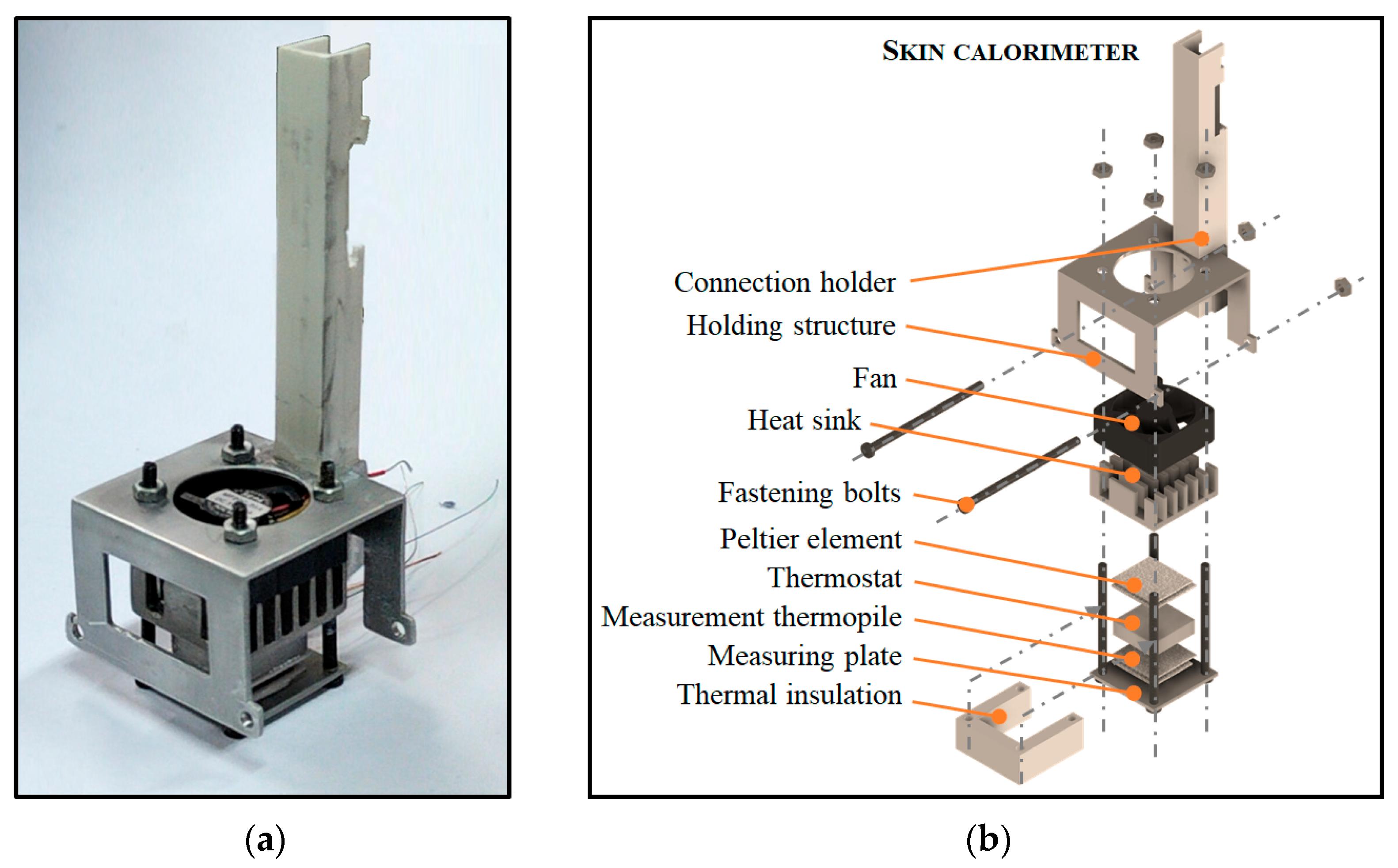
2.1. Skin Calorimeter

The skin calorimeter has two main components: the measuring thermopile and the thermostat. The measuring thermopile (ET12-65-F2A-1312-11-W2.25, Laird Thermal Systems, Morrisville, NC, USA) is placed between a 20 × 20 × 1 mm³ aluminum plate and a 14 × 14 × 4 mm³ aluminum block (the thermostat). The thermostat includes a PT100 temperature sensor (PT100GO1020HG, Omega Engineering, Norwalk, CT, USA) and a heating resistor (TFCC-005-50 by Omega Engineering, Norwalk, CT, USA). A cooling system, consisting of another thermopile (identical to the measuring one), an aluminum pin-fin heatsink (20 × 20 × 7 mm³), and a fan (MF20C05L-011, SEPA, Germany), is attached to the thermostat (Figure 1).

The thermopile, the thermostat, and the cooling thermopile are laterally insulated with expanded polystyrene (EPS) and finished with a reflective aluminum sheet. Two prototypes were built. Additionally, a calibration base was constructed using two small 10 × 10 × 4 mm³ aluminum blocks, each containing an electrical resistor for calibrating the calorimeters (TFCC-005-50 by Omega Engineering, Norwalk, CT, USA).

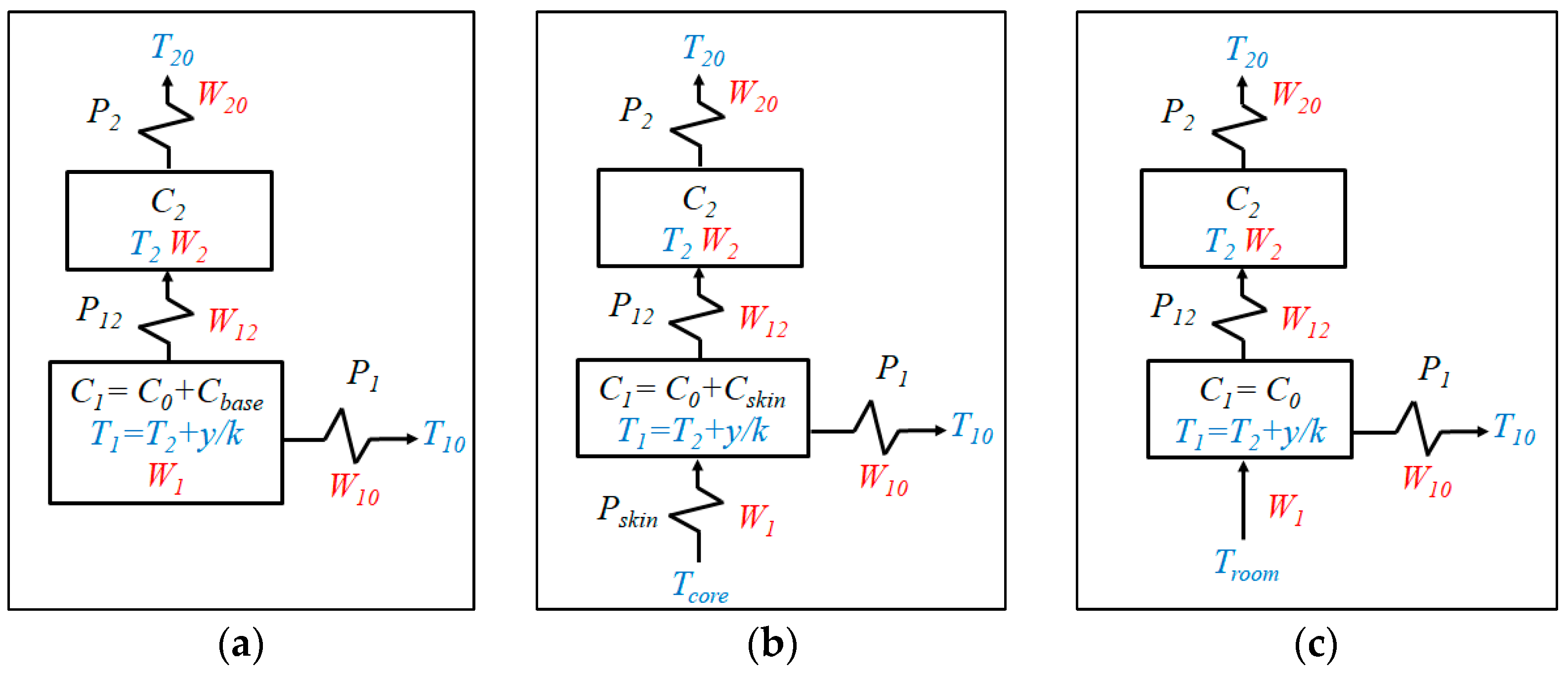
2.2. Calorimetric Model

The calorimetric model is based on an RC approach, as described in the introduction. This approach consists of decomposing the experimental system into N domains, each with a heat capacity C_i, thermally coupled to the neighboring domains by thermal conductances P_ik. The heat conduction equation for each domain is given by:

$$W_i(t)=C_i{\displaystyle \frac{d{T}_i(t)}{dt}}+{\displaystyle \sum _{k\ne i}^N{P}_{ik}(T_i-T_k)}+P_i(T_i-T_{0i})\hspace{0.17em}\hspace{0.17em}\hspace{0.17em}\hspace{0.17em}\mathrm{for} \hspace{0.17em}i=1\hspace{0.17em}\hspace{0.17em}to\hspace{0.17em}N$$

(2)

The underlying hypothesis is that each domain has infinite thermal conductivity, so the domain temperature can be considered spatially uniform. Under this assumption, the power developed (W_i) in a given domain equals the power required to change its temperature, C_idT_i/dt, plus the sum of the conduction heat losses to the neighboring domains, which are at a temperature T_k, including the external environment, which is at T_0i.

The calorimetric model consists of two domains with heat capacities C₁ and C₂, connected by a thermal conductance P₁₂. The domain temperatures, T₁ and T₂, are time-dependent. Each domain is connected to the outside through thermal conductances P₁ and P₂. The external temperatures are T₀₁ and T₀₂ (see Figure 2). The model equations are:

$$\begin{array}{l}{W}_1=C_1{\displaystyle \frac{d{T}_1}{dt}}+P_{12}(T_1-T_2)+P_1(T_1-T_{01})\\ W_2=C_2{\displaystyle \frac{d{T}_2}{dt}}+P_{12}(T_2-T_1)+P_2(T_2-T_{02})\end{array}$$

(3)

The calorimetric signal provided by the thermopile is proportional to the temperature difference between the domains, according to the Seebeck effect: y = k·(T₁ – T₂), where k is the Seebeck coefficient. Based on this relationship, the model can be formulated as follows:

$$\begin{array}{l}{W}_1={\displaystyle \frac{C_1}{k}}{\displaystyle \frac{dy}{dt}}+{\displaystyle \frac{P_1+P_{12}}{k}}y+C_1{\displaystyle \frac{d{T}_2}{dt}}+P_1(T_2-T_{01})\\ W_2=-{\displaystyle \frac{P_{12}}{k}}y+C_2{\displaystyle \frac{d{T}_2}{dt}}+P_2(T_2-T_{02})\end{array}$$

(4)

The inputs are the powers generated in each domain (W₁ and W₂), and the outputs are the calorimetric signal (y) and the thermostat temperature (T₂).

The first domain comprises the heat source, the measuring plate, and the external layer of the measuring thermopile. During calibration, the heat source is the calibration base, and the power dissipated is W₁. When the device is applied to the skin, W₁ represents the power transmitted from the skin to the calorimeter. The direction of the heat flux depends on the temperatures of the skin and the thermostat. The heat capacity of this domain is split into two components: the first corresponds to the calorimeter itself, denoted as C₀; the second corresponds to the small aluminum block containing the calibration resistor (C_base) or to the portion of the skin thermally excited by the calorimeter (C_skin). When the calorimeter is exposed to air, the heat capacity measured is nearly C₀, and the power W₁ corresponds to either incoming or outgoing heat flux, depending on the temperatures of the ambient and the thermostat.

Figure 2 shows a schematic representation of the calorimeter’s operation in the three cases described above.

The second domain represents the thermostat and the internal layer of the measuring thermopile. The power W₂ developed in this domain corresponds to the heat dissipated by the heating resistor inside the thermostat. This power is regulated by a proportional–integral (PI) controller to maintain the thermostat at the programmed temperature T₂.

The temperatures outside the calorimeter are influenced by the cooling system. Due to the Peltier effect, the temperature T₀₂ of the thermostat side in contact with the cooling thermopile decreases, while the temperature of the opposite side increases. As a result, the heat sink and the fan must evacuate this heat, causing the external temperature T₀₁ to rise. Both T₀₁ and T₀₂ depend on the supply current I_pel and the ambient temperature. The ambient temperature measured is T_room, but the temperature in the proximity of the sensor is slightly different due to the local cutaneous warming effect, represented by T₀. Experimental measurements confirmed that these relationships are linear up to I_pel = 0.21 A.

$$\begin{array}{l}{T}_{01}=T_{room}+T_0+\alpha I_{pel}\\ T_{02}=T_{room}+T_0+\beta I_{pel}\end{array}$$

(5)

2.3. Measurement and Control System

A data acquisition system (Keysight 34970A and module 34901A, Santa Rosa, CA, USA) records the calorimetric signal, as well as the ambient and thermostat temperatures. The electrical inputs and the cooling thermopile current are supplied by a programmable triple-output power supply (Keysight E3631A, Santa Rosa, CA, USA). Instrument control and data collection are managed through a C++ program via a GPIB interface (Keysight 82357B, Santa Rosa, CA, USA), with a sampling period of ∆t = 1 s.

2.4. Identification of Model Parameters

To assess the behavior of the calorimetric system under different conditions, a series of programmed thermostat temperature changes was performed.

The estimation of the model parameters C₁, C₂, P₁, P₂, P₁₂, and k consists of an optimization process based on the Nelder–Mead simplex algorithm [28], with the Lagarias improvement [29], which provide a more rigorous convergence analysis and increased robustness compared to the original Nelder–Mead algorithm. This algorithm compares the model’s predicted outputs with the experimental data. By applying an iterative method, the model generates ∆y and ∆T₂ values from the input signals ∆W₁ and ∆W₂, using the model equations (Equation (4)). The fitting process minimizes the root mean square error (RMSE) (Equation (6)) across both output variables, which is the objective function to minimize in the algorithm. This process is implemented by MATLAB’s fminsearch function [30]. To ensure reliable identification, each experiment is conducted under thermally stable conditions. Both the ambient temperature and the cooling current remain constant during the measurement, which allows the assumption that external temperatures T₀₁ and T₀₂ do not vary significantly. This enables signal baseline correction and ensures consistent initial and final states.

$$\epsilon ={\displaystyle \frac{1}{n}}\sqrt{{\displaystyle \sum _{i=1}^n{\left(y_{\exp }-y_{cal}\right)}^2}}+{\displaystyle \frac{1}{n}}\sqrt{{\displaystyle \sum _{i=1}^n{\left({T_2}_{\exp }-T_{2cal}\right)}^2}}={\epsilon }_y+{\epsilon }_{T_2}$$

(6)

where ε_y and ε_T2 are the RMSE of the output signals and n is the number of data points.

Table 2. RC model (Equation (4)) and cooling system (Equation (5)) parameters.

	Calorimeter S1	Calorimeter S2
Parameters	Mean ± std	Mean ± std	Units
RC model
C0	2.31 ± 0.07	2.31 ± 0.07	J/K
C1	4.02 ± 0.09	3.91 ± 0.09	J/K
C2	3.8 ± 0.2	3.7 ± 0.3	J/K
P1	0.029 ± 0.002	0.029 ± 0.002	W/K
P2	0.057 ± 0.005	0.055 ± 0.005	W/K
P12	0.092 ± 0.008	0.089 ± 0.009	W/K
k	23.7 ± 1.1	23.0 ± 1.4	mV/K
Cooling system
α 1	13.6	17.4	°C/A
β 1	–83.5	–83.8	°C/A
T0 2	0.45	0.36	°C
RMSE values
εy	16.5 ± 2.5	16.2 ± 2.4	µV
εT2	3.9 ± 2.0	3.8 ± 2.0	mK

A total of 35 calibration measurements were performed, each one lasting 30 min. ¹ Pearson coefficient (r) was higher than 0.97 in all cases, and Spearman coefficient higher than 0.98. ² Note that T₀ has been determined when the calorimeter is placed on the calibration base. However, when the calorimeter is placed on the skin, its value is higher due to the proximity to the human body, and therefore this parameter is not invariant and has to be determined for each experiment.

shows the RC model parameters of each calorimeter. It should be noted that all model parameters are constant except C₁, which varies depending on the heat capacity of the sample analyzed. However, a portion of C₁ is invariant and intrinsic to the calorimeter itself; this value is denoted as C₀. To determine this heat capacity, we conducted measurements similar to those described above, but with the calorimeter exposed directly to air.

Although this process achieves accurate identification, the initial and final values of W₁ are lost because the baseline has been corrected. To complete the model calibration and enable the assessment of the initial and final values of all signals, it is necessary to incorporate the effects of the cooling system into the model. If baseline correction is omitted, the model can be fitted by incorporating the equations that describe the cooling effects (Equation (5)), thus allowing the estimation of parameters α, β, and T₀, which are listed in Table 2. The term α·I_pel represents the increase in temperature around the calorimeter due to heating of the heat sink, ranging from 0 to 4 °C. In contrast, the term β·I_pel represents the cooling of the cold side of the thermopile (in contact with the thermostat) due to the Peltier effect, ranging from 0 to –18 °C. We have verified that these temperature changes are linear with I_pel, as indicated by the Spearman (ρ > 0.98) and the Pearson (r > 0.97) coefficients.

To conclude this section, we define a transfer function (TF) that relates the variation of the calorimetric signal (∆y) to the variation of the power input (∆W₁). This relationship is derived from the first equation of the model (Equation (2)), under the assumption that the thermostat temperature is constant. The resulting TF enables comparison of the sensitivities of different heat flux sensors (HFSs), as summarized in Table 1. Our skin calorimeter has a sensitivity of K = 195.5 mV/W, which is higher than that of conventional HFSs. Regarding the time constant τ, it depends on the heat capacity of the sample under analysis. When the calorimeter is exposed to air, the time constant is 20 s, significantly higher than that of thin-film HFSs, which typically exhibit time constants around 1 s. As expected for a calorimetric instrument, it provides higher measurement accuracy at the cost of a slower response time.

$$TF(s)={\displaystyle \frac{\Delta Y(s)}{\Delta W_1(s)}}={\displaystyle \frac{\left(\frac{k}{P_1+P_{12}}\right)}{1+s\left(\frac{C_1}{P_1+P_{12}}\right)}}={\displaystyle \frac{K}{1+s\tau }}$$

(7)

3. Results

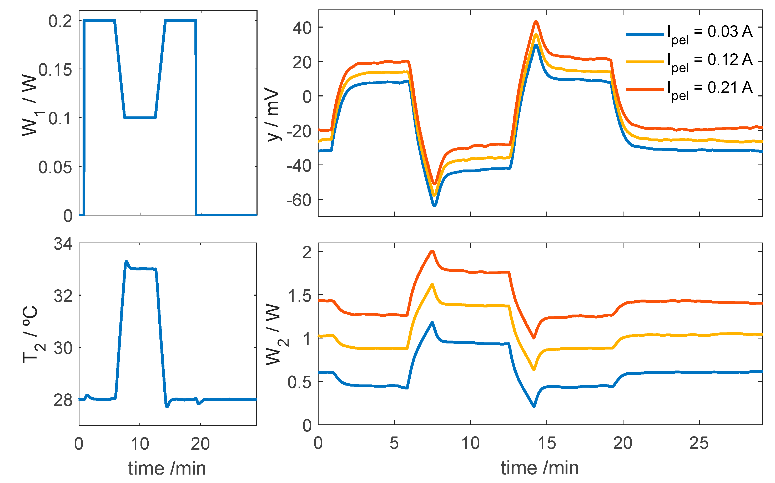
3.1. Parameters of the Calorimetric Model

In this subsection, we perform an application of the procedure described in Section 2.4. Each experiment began by stabilizing the thermostat at 28 °C to establish thermal equilibrium. The temperature was then increased to 33 °C at a rate of 3 K/min, held steady for 5 min, and reduced back to 28 °C at the same rate. During this thermal cycle, a variable heating profile was applied to the calibration base: an initial input of 0.2 W was decreased to 0.1 W during the high-temperature phase, restored to 0.2 W afterward, and finally turned off. This protocol was repeated for different values of the cooling thermopile current, ranging from 0.03 A to 0.21 A. Figure 3 shows representative results for the lowest, highest, and an intermediate I_pel value. The experiment was conducted at a room temperature of 21 °C.

3.2. Simulations

Experimental testing of calorimetric systems can be slow, costly, and technically complex, especially when dealing with biological samples or long-duration measurements. In this context, simulations can reproduce the system’s behavior under different conditions, helping to reduce experimental effort. In this work, we present three main applications:

• PI controller and thermal regulation: simulations allow the PI controller parameters to be adjusted and to verify that the thermostat temperature accurately follows the programmed thermal profile;
• Calorimetric response under resting conditions: simulations are used to analyze the behavior of the calorimeter when it is applied to the skin at rest;
• Calorimetric response during physical activity: Simulations also allow evaluation of the response when the subject performs physical exercise, which generates transient heat fluxes.

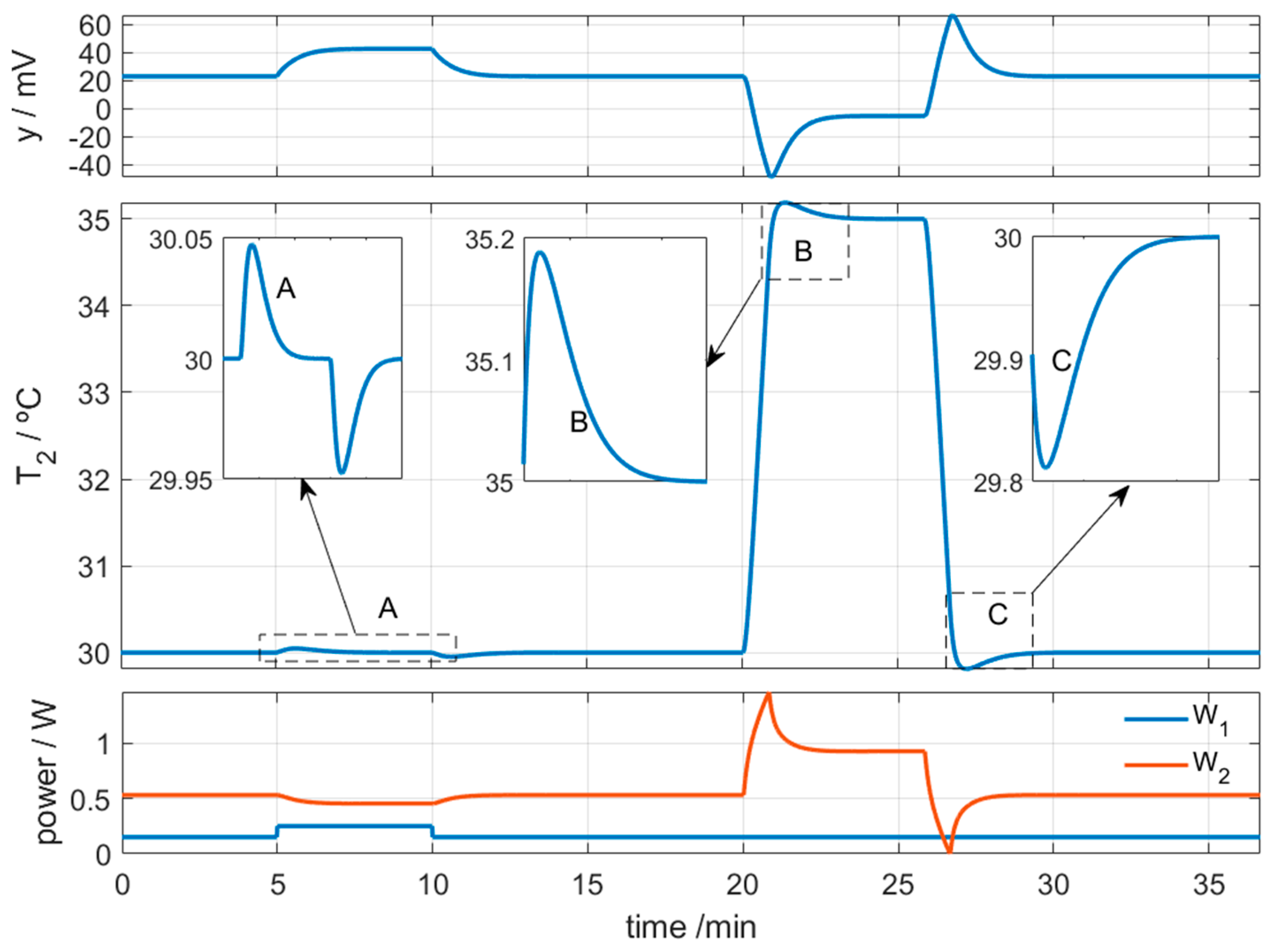
3.2.1. Control of Thermostat Temperature

Temperature control is performed by a PI controller that determines the power W₂ to be dissipated in the resistor placed in the thermostat, in order to achieve the programmed temperature T_2REF (t):

$$\begin{array}{l}{W}_2(t)=k_p\epsilon (t)+k_i{\displaystyle \int \epsilon (t)dt}\\ \epsilon (t)=T_{2REF}(t)-T_2(t)\end{array}$$

(8)

The experimental values of temperature T₂ are measured using the PT100 sensor placed inside the thermostat. The dissipated power W₂ is limited between zero and a maximum value, which is 2 W in these calorimeters.

The operating domain of the calorimeter is defined by the maximum and minimum thermostat temperatures that can be programmed during a measurement. When the thermostat fails to reach the programmed temperature, the system enters saturation; that is, the power W₂ dissipated in the thermostat’s heating resistor exceeds the specified power limits. Figure 4 shows a schematic of the temperature control system. It illustrates how the thermostat temperature is influenced by the ambient temperature, the cooling thermopile current, and the power inputs W₁ and W₂.

The PI controller parameters were determined according to the following requirements: (1) for a disturbance of ∆W₁ = 100 mW, the thermostat temperature deviation must remain below 0.05 °C; and (2), for a programmed temperature step of 6 K/min, the overshoot must be less than 5%. These criteria reflect the common operating conditions for skin applications. The first requirement corresponds to a cutaneous heat flux change that may occur, for instance, during physical exercise. Regarding the second requirement, a controlled variation in thermostat temperature is required to determine the heat capacity and the thermal resistance of the skin, and saturation must be avoided. Under these specifications, we obtained k_p = 0.5 WK⁻¹ and k_i = 0.02 WK⁻¹s⁻¹.

Figure 5 shows a simulation in which W₁ is initially 150 mW, then increases to 250 mW, and subsequently returns to 150 mW. During this interval, the thermostat temperature—programmed at 30 °C—exhibits a maximum disturbance of 0.05 °C (see zoom plot A in Figure 5). In the same simulation, the thermostat temperature is increased from 30 °C to 35 °C at a rate of 6 K/min, with an overshoot of 0.2 °C, remaining within the 5% limit (see zoom plots B and C in Figure 5). This simulation was performed for an ambient temperature of T_room = 25 °C and a cooling system supply current of I_pel = 0.1 A.

On the other hand, the simulations also allow the adjustment of the cooling system supply current to prevent saturation during a given thermostat temperature change. As an example, we consider a thermostat temperature setting from 30 to 35 °C (6 K/min), with a constant dissipation of W₁ = 150 mW, and different room temperatures. In the first case, for a room temperature of T_room = 25 °C and I_pel = 0.1 A, the temperature control works adequately (Figure 6A). However, for a T_room = 30 °C and I_pel = 0.1 A, lower saturation of the thermostat power occurs, leading to a return to the initial temperature with higher overshoot and longer stabilization time (Figure 6B). For this room temperature (T_room = 30 °C), it is necessary to decrease the cold focus temperature by increasing the Peltier power supply (I_pel = 0.2 A), and now we observe that the control works adequately (Figure 6C).

In summary, the operating domain depends on the ambient temperature, the power W₁ that passes through the calorimeter, the thermostat temperature settings, and the cooling system. As many variables are involved, simulations are necessary to ensure that the thermostat power will not enter saturation for a given experiment.

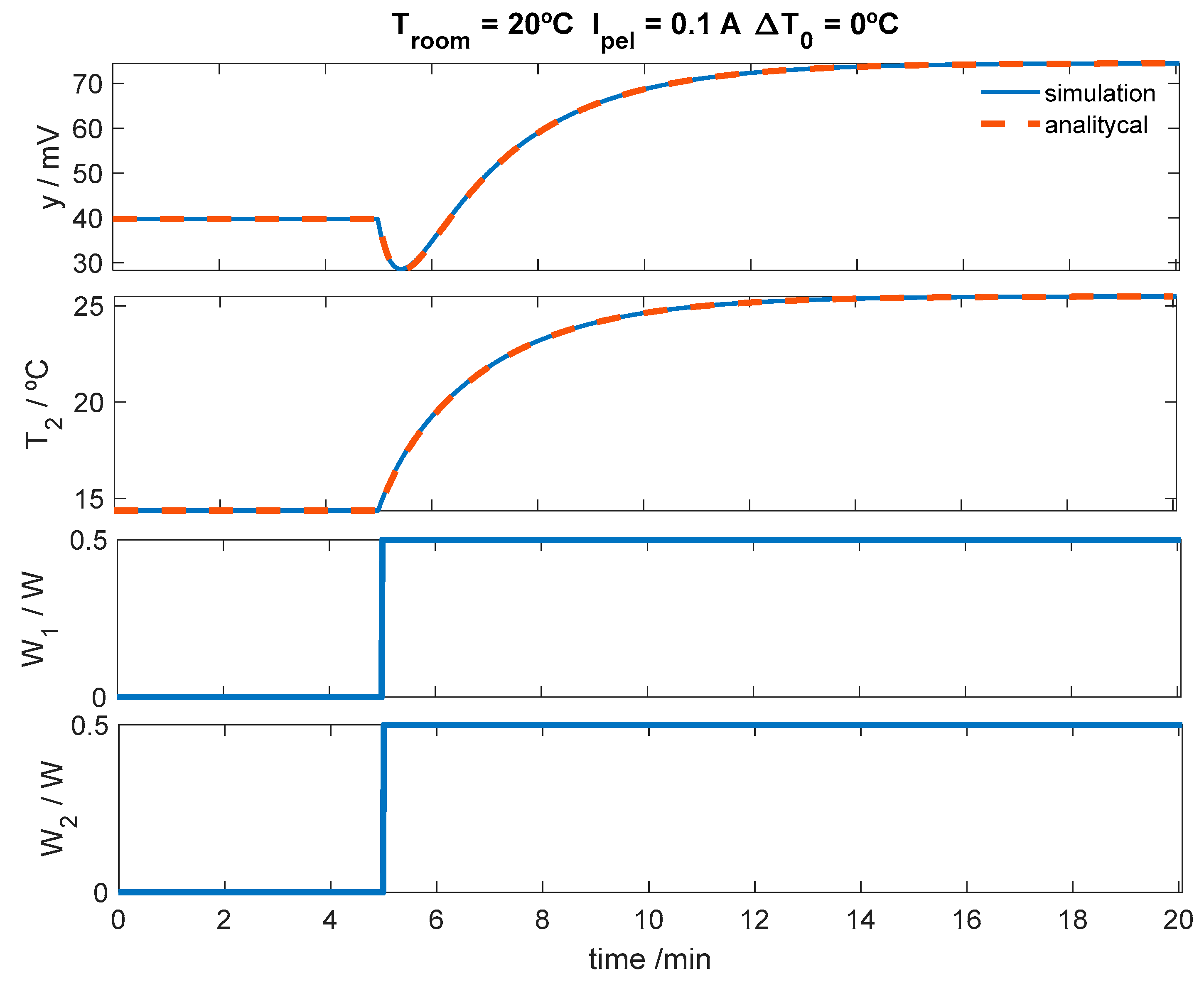
3.2.2. Simulation of the Calorimeter’s Operation for Skin Application at Rest

According to the model scheme shown in Figure 2, when the calorimeter is applied to the skin, the power W₁ transmitted from the inside of the human body to the calorimeter, through the skin’s thermal conductance P_skin, is given by the following expression:

$$W_1=\left(T_{core}-T_1\right)P_{skin}=\left(T_{core}-T_2-{\displaystyle \frac{y}{k}}\right)P_{skin}$$

(9)

where T_core is the core temperature in the region where the measurement is taken, and T₁ is the temperature of the first domain of the calorimetric model, which has a heat capacity C₁ = C₀ + C_skin. The measured variables are the thermostat temperature (T₂) and the calorimetric signal (y). By including this expression in the calorimetric model equation, we obtain Equation (10), which describes the behavior of the calorimeter when it is placed on the skin:

$$\begin{array}{l}{T}_{core}{P}_{skin}={\displaystyle \frac{C_1}{k}}{\displaystyle \frac{dy}{dt}}+{\displaystyle \frac{P_1+P_{12}+P_{skin}}{k}}y+C_1{\displaystyle \frac{d{T}_2}{dt}}+(P_1+P_{skin})T_2-P_1{T}_{01}\\ W_2=-{\displaystyle \frac{P_{12}}{k}}y+C_2{\displaystyle \frac{d{T}_2}{dt}}+P_2(T_2-T_{02})\end{array}$$

(10)

Using this model, we simulate the operation of the calorimeter on human skin at rest. We consider a skin thermal resistance of R_skin = 25 K/W, room temperatures of 20 °C and 24 °C, and a cooling current of 0.08 A. The thermostat temperature is varied from 28 °C to 37 °C at a rate of 6 K/min in three 3K intervals. This thermostat temperature variation induces changes in the heat fluxes transmitted through the calorimeter, and consequently, variations in the temperature T₁ of the first domain of the model. Since the subject is at rest, no significant changes are expected in the core temperature of the region where the calorimeter is applied. In this simulation, we consider a lower limb with an internal core temperature T_core = 33 °C. When the calorimeter is applied to the skin, the proximity of the human body increases the local temperature around the device. This effect is modeled by the parameter T₀ in Equation (5), which in this case is T₀ = 2.5 °C.

Figure 7 shows the simulation results for the case of T_room = 24 °C.

Table 3. Temperatures (ºC) and heat fluxes (in W) from a simulation of the calorimeter–skin system when the thermostat temperature (T₂) is varied and the subject is at rest (see Figure 7). The sign convention used is that shown in Figure 2 (W₂ is always positive). I_pel = 0.08 A; T₀ = 2.5 °C (see Equation (5)). The core temperature considered was T_core = 33 °C.

Troom	T1	T01	T2	T02	W1	W10	W12	W2	W20
20	28.448	23.59	28	15.820	0.18210	0.1409	0.0412	0.6531	0.6943
20	30.162	23.59	31	15.820	0.11353	0.1906	−0.0771	0.9424	0.8653
20	31.876	23.59	34	15.820	0.04496	0.2404	−0.1954	1.2317	1.0363
20	33.590	23.59	37	15.820	−0.02362	0.2901	−0.3137	1.5209	1.2072
24	29.168	27.59	28	19.820	0.15328	0.0458	0.1075	0.3588	0.4663
24	30.882	27.59	31	19.820	0.08471	0.0955	−0.0108	0.6481	0.6373
24	32.597	27.59	34	19.820	0.01613	0.1452	−0.1291	0.9374	0.8083
24	34.311	27.59	37	19.820	−0.05243	0.1950	−0.2474	1.2267	0.9793

lists the heat fluxes for both ambient temperatures (20 and 24 °C). The sign convention is defined in Figure 2, and the results show consistency with the temperatures T_core, T₁, T₀₁, T₂, and T₀₂. Although the heat fluxes depend on the ambient temperature, the ratio ∆T₁/∆W₁ remains constant, independent of both ambient temperature and the thermostat programming. For the 3 K thermostat steps programmed, we obtain ∆T₁ = 1.7143 K, ∆W₁ = 0.06858 W, and ∆T₁/∆W₁ ≈ 25 K/W in all cases.

There are two important results from the simulation. The first is the relationship between the heat flux (W₁) and the thermostat temperature (T₂). The second is the definition of the skin’s thermal resistance (R_skin). These are described as follows:

$$\begin{array}{l}{W}_1(t)=W_1(0)-\Delta W_1{\displaystyle \frac{T_2(t)-T_2(0)}{\Delta T_2}}\\ R_{skin}={\displaystyle \frac{\Delta T_1}{\Delta W_1}}={\displaystyle \frac{\Delta T_2+\Delta y/k}{\Delta W_1}}\end{array}$$

(11)

In the first expression, T₂ (t) is the thermostat temperature, T₂ (0) is its initial steady-state value, and ∆T₂ is the maximum temperature increase. W₁ (0) is the initial steady-state cutaneous heat flux corresponding to T₂ (0), and ∆W₁ is the variation in heat flux associated with ∆T₂. The simulation shows that the first expression provides a good approximation of the cutaneous heat flux in steady state, although it does not fully capture the transient response. However, the approximation is accurate enough to determine ∆W₁ in steady state. Figure 8 shows the cutaneous heat flux computed using Equation (11), compared with the one obtained from the simulation. Regarding the second expression in Equation (11), the simulation confirms that this thermal resistance is invariant and does not directly depend on ambient temperature or the thermostat temperature settings.

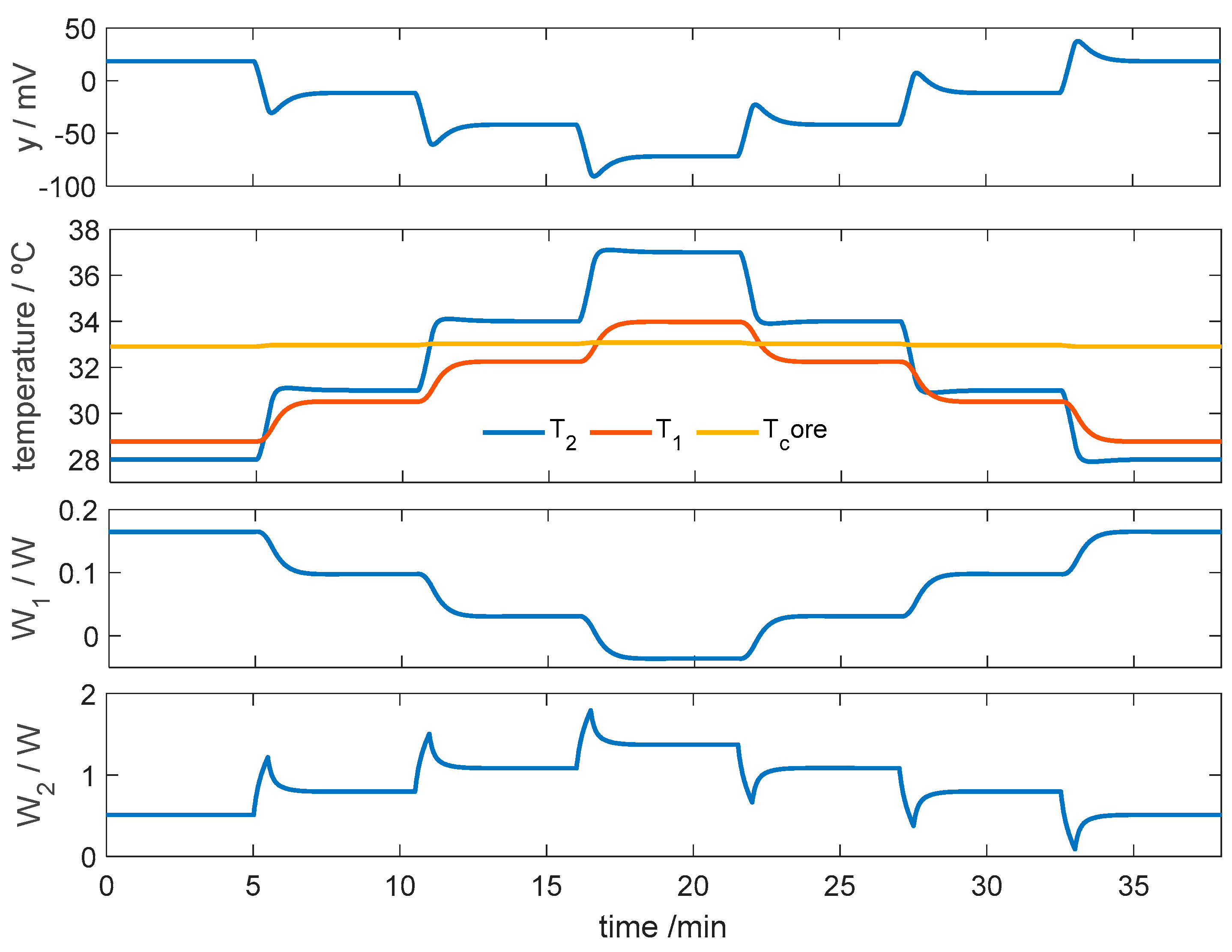
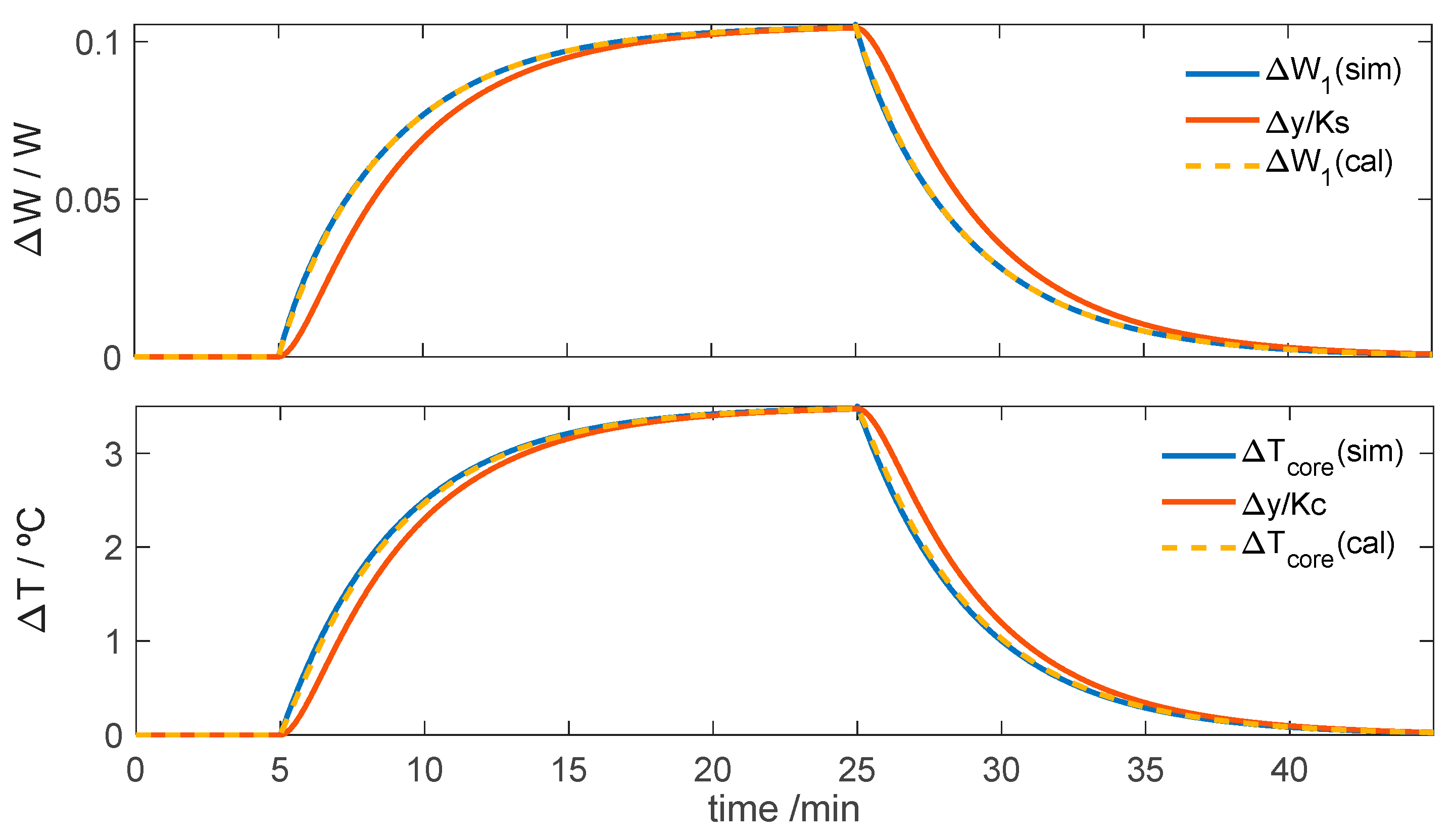
3.2.3. Simulation of the Calorimeter’s Operation for Skin Application During Exercise

The last simulation reproduces the case of a subject performing physical exercise. In a previous study, we experimentally measured the response of the calorimeter when it was applied to the thigh of a healthy 28-year-old male subject performing moderate exercise on a stepper [17]. In that experiment, the thermostat temperature was set to a constant value, and after an initial steady state was reached, the exercise session began. Signals were also recorded after the exercise ended, in order to analyze the subject’s recovery phase. The study showed that, during exercise, the cutaneous heat flux increased by 100 mW at a constant thermostat temperature of 26 °C. Based on these experimental results, we simulated the skin–calorimeter system during exercise.

We assume that the heat flux increase is caused by a significant T_core rise. This increase, as well as its subsequent decrease, is modeled as an exponential process. Based on the experimental data cited in the previous paragraph, we consider a time constant of 4 min for both heating and cooling phases. The initial core temperature is set to 33 °C, with an exponential increase of ΔT_core = 3.5 °C. The simulation is performed for different constant thermostat temperatures (T₂ = 25, 30, and 35 °C), at an ambient temperature of T_room = 24 °C. The exercise lasts for 20 min and begins at t = 5 min. Figure 9 shows the results of the proposed simulation: the calorimetric signal, the temperatures T_core, T₁, and T₂, the cutaneous heat flux W₁, and the thermostat power W₂ required to maintain the thermostat temperature constant.

This study shows that the calorimetric response and the heat fluxes depend on the ambient temperature, the current supplied to the cooling thermopile, and the thermostat temperature. However, variations in the calorimetric signal (Δy) and in the heat flux (∆W₁) remain the same for a given core temperature variation (∆T_core). Therefore, when the thermostat temperature is kept constant, the heat flux variation can be determined using the transfer function given in Equation (7), by applying a derivative filter to the baseline-corrected calorimetric signal:

$$\Delta W_1={\displaystyle \frac{1}{K_s}}\left(\Delta y+{\tau }_s{\displaystyle \frac{d\Delta y}{dt}}\right)$$

(12)

In this case, the sensitivity value is K_s = k/(P₁ + P₁₂) = 196 mV/W, and the time constant value is τ_s = C₁/(P₁ + P₁₂), which depends on the heat capacity of the portion of skin that has been thermally excited. In this simulation, C₁ = 6 J/K and τ_s = 49.6 s.

In a similar way, the core temperature variation can be directly obtained using an analogous expression derived from the first term of Equation (10):

$$\Delta T_{core}={\displaystyle \frac{1}{K_c}}\left(\Delta y+{\tau }_c{\displaystyle \frac{d\Delta y}{dt}}\right)$$

(13)

In this case, the sensitivity is K_c = k/(P₁ + P₁₂ + P_skin) = 5.9 mV/K, and the time constant is τ_c = C₁/(P₁ + P₁₂ + P_skin) = 33.7 s.

With the identification of the calorimeter–skin system and knowledge of the calorimetric signal, two key quantities can be determined: the variation in heat flux and the core temperature. Figure 10 shows both the simulated curves (solid lines) and the calculated curves (dashed lines).

Finally, it is of interest to determine the absolute core temperature of the skin in the region where the calorimeter is applied. Under steady-state conditions, this temperature can be obtained from the following expression:

$$\begin{array}{l}{T}_{core}={\displaystyle \frac{P_1+P_{12}+P_{skin}}{k\hspace{0.17em}{P}_{skin}}}y+{\displaystyle \frac{(P_1+P_{skin})}{P_{skin}}}{T}_2-{\displaystyle \frac{P_1}{P_{skin}}}(T_0+T_{room}+\alpha I_{pel})=\\ \hspace{0.17em}\hspace{0.17em}\hspace{0.17em}\hspace{0.17em}\hspace{0.17em}\hspace{0.17em}\hspace{0.17em}\hspace{0.17em}\hspace{0.17em}\hspace{0.17em}\hspace{0.17em}=0.1698 y+1.725 T_2-0.725 T_{01}\end{array}$$

(14)

In this expression, all parameters and variables are known except for T_core and the temperature increase around the calorimeter, T₀. The value of T₀ can be determined from the second expression of the model for the steady-state condition. In this second expression, all parameters and variables are known except for T₀:

$$W_2=-{\displaystyle \frac{P_{12}}{k}}y+P_2(T_2-T_0-T_{room}-\beta I_{pel})$$

(15)

Table 4. Initial steady-state values from the simulation (Figure 9): calorimetric signal (y), thermostat and external temperatures (T₂ and T₀₁), and core temperature (T_core), calculated using Equation (14).

y/mV	T2/°C	T01/°C	Tcore/°C
59.31	25.0	27.86	33.0
8.53	30.0	27.86	33.0
–42.26	35.0	27.86	33.0

shows the values of the variables used to determine the core temperature, T_core. As can be seen, Equation (14) enables this temperature to be accurately determined.

In summary, the most relevant variables obtained during the exercise are the core temperature (Equation (14)) and its variations (Equation (12)), as well as the cutaneous heat flux (Equation (13)), which can be easily determined using the corresponding expressions.

4. Discussion

The first results presented in this work correspond to the identification of the calorimetric model parameters (Table 2). During calibration, we found good agreement between the experimental results and the model simulations for different operating modes of the calorimeter (Figure 2). Under normal operation, the cooling thermopile current (I_pel) is kept constant, so the device can be considered a two-input, two-output system. The inputs are the heat flux (W₁) and the power (W₂) dissipated in the thermostat, and the outputs are the calorimetric signal y(t) and the thermostat temperature (T₂). The model’s differential equations were solved numerically using the finite difference method, with a time step equal to the experimental sampling period (Δt = 1 s). This approach facilitates implementation in the acquisition and control program for the calorimeters, which is written in C++. To check the method’s accuracy, we analyzed the response to two simultaneous step inputs. Figure 11 shows the calorimetric response (y) and the thermostat temperature (T₂) from both the simulation and the analytical solution (Equation (16)). The figure also shows the input signals, each with a power value of 0.5 W.

$$\begin{array}{l}y(t)=y_0+{\displaystyle \sum _{i=1}^2{W}_i}{\displaystyle \sum _{j=1}^2{a}_{ij}}\left(1-\exp \left(-t/{\tau }_j\right)\right)\\ T_2(t)=T_{20}+{\displaystyle \sum _{i=1}^2{W}_i}{\displaystyle \sum _{j=1}^2{b}_{ij}}\left(1-\exp \left(-t/{\tau }_j\right)\right)\end{array}$$

(16)

The maximum deviation between the simulated calorimetric signal and that obtained from the analytical expression is 0.2 mV (0.4% of the signal step change), and the maximum deviation in the thermostat temperature is 0.01 °C (0.1% of the temperature step change). Considering that the experimental noise of the calorimetric signal in steady state is ±0.3 mV and the thermostat temperature fluctuates by ±0.01 °C, we consider the simulation results acceptable.

On the other hand, simulations of the skin calorimeter were performed in two different situations. In the first case, measurements were conducted on a subject at rest, which allows the determination of the heat capacity and the thermal resistance of a localized area of the skin. These results have two particularly interesting applications. First, knowing the internal thermal resistance of the skin makes it possible to estimate the internal temperature. Second, both parameters can be used to monitor skin lesions. This application was studied in a recent work [31] by measuring two symmetrical areas on the dorsal side of the wrist, one of which had suffered a second-degree burn. Monitoring these properties enabled the study of the temporal recovery of the lesion. In the introduction of this work, other instruments [5,7,8,10,12] were referenced, all aimed at measuring the thermal properties of the skin and studying possible anomalies, but always in subjects at rest. The skin calorimeter presented in this study opens up a new application by measuring local heat flux in subjects during exercise.

The second case studied involves a subject performing physical exercise. We are actively working in this area, and for moderate exercise, our experimental measurements have shown very promising results for monitoring muscle heat flux over time. The improvement of these calorimeters [15,16,17], along with the accurate measurement of transmitted heat fluxes and the acquisition of new experimental data in humans, is leading to new approaches for the detailed study of the thermal behavior of muscles involved in physical activity. Currently, we are developing models that explain variations in heat flux as a function of mechanical work, blood flow, and sweating during exercise. Sweating causes a reduction in transmitted heat flux. Although this may seem like a limitation of the instrument, this phenomenon can be detected during measurement and incorporated into the thermal behavior model of the measured area. This discussion shows that the simulation accurately reproduces the instrument’s operation and highlights the need for further experimental measurements in exercising subjects to propose and evaluate models of thermal behavior.

5. Conclusions

This work presents and validates an RC model of a skin calorimeter, capable of providing medically relevant parameters in both resting and exercising subjects. We conclude the following:

A functional model of the calorimeter–skin system has been proposed, applicable to both calibration scenarios and real measurements on human skin. The parameters of the model have been identified, and simulations have been carried out to evaluate both temperature control and the performance of the calorimeter when applied to the skin of a subject at rest and during physical exercise.

For the resting case, the method and proposed expressions allow the determination of the heat flux, the heat capacity, the thermal resistance, and the core temperature of the skin area under study. For the exercising case, the proposed expressions allow the simple estimation of the variation of the core temperature and cutaneous heat flux of the region under study.

The simulations validate the proposed expressions and enable the evaluation of heat fluxes through the calorimeter under different thermostat and ambient temperatures. In summary, the device provides access to physiologically relevant quantities such as skin heat capacity, thermal resistance, heat flux, and core body temperature. These can all be obtained non-invasively from a localized region of the human body using this skin calorimeter, which has a contact area of 2 × 2 cm².

References

1. Available online: https://sea.omega.com/th/pptst/HFS-3_HFS-4.html#description (accessed on 7 April 2025).
2. Available online: https://es.omega.com/pptst/UHF-HFS-SERIES.html#description (accessed on 7 April 2025).
3. Available online: https://www.hukseflux.com/products/heat-flux-sensors/heat-flux-sensors (accessed on 7 April 2025).
4. Tanaka, Y.; Matsunaga, D.; Tajima, T.; Seyama, M.; Kato, I.; Nagashima, K. Skin-Attachable Sensor for Continuous Core Body Temperature Monitoring. IEEE Sens. J. 2024, 24, 38708–38714. [Google Scholar] [CrossRef]
5. Okabe, T.; Fujimura, T.; Okajima, J.; Aiba, S.; Maruyama, S. Non-invasive Measurement of Effective Thermal Conductivity of Human Skin with a Guard-Heated Thermistor Probe. Int. J. Heat Mass Transf. 2018, 126, 625–635. [Google Scholar] [CrossRef]
6. Kharalkar, N.M.; Hayes, L.J.; Valvano, J.W. Pulse-Power Integrated-Decay Technique for the Measurement of Thermal Conductivity. Meas. Sci. Technol. 2008, 19, 075104. [Google Scholar] [CrossRef]
7. Madhvapathy, S.R.; Ma, Y.; Patel, M.; Krishnan, S.; Wei, C.; Li, Y.; Xu, S.; Feng, X.; Huang, Y.; Rogers, J.A. Epidermal Electronic Systems for Measuring the Thermal Properties of Human Skin at Depths of up to Several Millimeters. Adv. Funct. Mater. 2018, 28, 1802083. [Google Scholar] [CrossRef]
8. Zubiaga, A.; Kirsch, C.; Boiger, G.; Bonmarin, M. A Simple Instrument to Measure the Thermal Transport Properties of the Human Skin. In Proceedings of the 2021 IEEE International Symposium on Medical Measurements and Applications (MeMeA), Lausanne, Switzerland, 23–25 June 2021; pp. 1–5. [Google Scholar] [CrossRef]
9. Zhang, X.; Bontozoglou, C.; Xiao, P. In Vivo Skin Characterizations by Using Opto-Thermal Depth-Resolved Detection Spectra. Cosmetics 2019, 6, 54. [Google Scholar] [CrossRef]
10. Grenier, E.; Gehin, C.; McAdams, E.; Lun, B.; Gobin, J.-P.; Uhl, J.-F. Effect of Compression Stockings on Cutaneous Microcirculation: Evaluation Based on Measurements of the Skin Thermal Conductivity. Phlebology 2014, 31, 101–105. [Google Scholar] [CrossRef]
11. Wang, L.; Chong, D.; Di, Y.; Yi, H. A Revised Method to Predict Skin’s Thermal Resistance. Therm. Sci. 2018, 22, 1795–1802. [Google Scholar] [CrossRef]
12. Webb, R.C.; Pielak, R.M.; Bastien, P.; Ayers, J.; Niittynen, J.; Kurniawan, J.; Manco, M.; Lin, A.; Cho, N.H.; Malyrchuk, V.; et al. Thermal Transport Characteristics of Human Skin Measured In Vivo Using Ultrathin Conformal Arrays of Thermal Sensors and Actuators. PLoS ONE 2015, 10, e0118131. [Google Scholar] [CrossRef]
13. Webb, R.C.; Bonifas, A.P.; Behnaz, A.; Zhang, Y.; Yu, K.J.; Cheng, H.; Shi, M.; Bian, Z.; Liu, Z.; Kim, Y.S.; et al. Ultrathin Conformal Devices for Precise and Continuous Thermal Characterization of Human Skin. Nat. Mater. 2013, 12, 938–944. [Google Scholar] [CrossRef]
14. Gao, L.; Zhang, Y.; Malyarchuk, V.; Jia, L.; Jang, K.; Webb, R.C.; Fu, H.; Shi, Y.; Zhou, G.; Shi, L.; et al. Epidermal Photonic Devices for Quantitative Imaging of Temperature and Thermal Transport Characteristics of the Skin. Nat. Commun. 2014, 5, 4938. [Google Scholar] [CrossRef]
15. Rodríguez de Rivera, P.J.; Rodríguez de Rivera, M.; Socorro, F.; Rodríguez de Rivera, M. In Vivo Measurement of Skin Heat Capacity: Advantages of the Scanning Calorimetric Sensor. J. Therm. Anal. Calorim. 2022, 147, 12155–12163. [Google Scholar] [CrossRef]
16. Rodríguez de Rivera, P.J.; Rodríguez de Rivera, M.; Socorro, F.; Calbet, J.A.L.; Rodríguez de Rivera, M. Advantages of In Vivo Measurement of Human Skin Thermal Conductance Using a Calorimetric Sensor. J. Therm. Anal. Calorim. 2022, 147, 10027–10036. [Google Scholar] [CrossRef]
17. Rodríguez de Rivera, M.; Rodríguez de Rivera, P.J. New, Optimized Skin Calorimeter Version for Measuring Thermal Responses of Localized Skin Areas during Physical Activity. Sensors 2024, 24, 5927. [Google Scholar] [CrossRef]
18. Carslaw, H.S.; Jaeger, J.C. Conduction of Heat in Solids; Clarendon-Press: Oxford, UK, 2008. [Google Scholar]
19. Wissler, E.H. Pennes’ 1948 Paper Revisited. J. Appl. Physiol. 1998, 85, 35–41. [Google Scholar] [CrossRef]
20. Lakhssass, A.; Kengne, E.; Semmaoui, H. Modified Pennes’ Equation Modeling Bio-Heat Transfer in Living Tissues: Analytical and Numerical Analysis. Nat. Sci. 2010, 2, 1375–1385. [Google Scholar] [CrossRef]
21. Deng, Z.S.; Liu, J. Blood Perfusion-Based Model for Characterizing the Temperature Fluctuation in Living Tissues. Physica A 2001, 300, 521–530. [Google Scholar] [CrossRef]
22. Sarkar, D.; Haji-Sheikh, A.; Jain, A. Temperature Distribution in Multi-Layer Skin Tissue in Presence of a Tumor. Int. J. Heat Mass Transf. 2015, 91, 602–610. [Google Scholar] [CrossRef]
23. Agrawal, M.; Pardasani, K.R. Finite Element Model to Study Temperature Distribution in Skin and Deep Tissues of Human Limbs. J. Therm. Biol. 2016, 62, 98–105. [Google Scholar] [CrossRef] [PubMed]
24. Rodríguez de Rivera, P.J.; Rodríguez de Rivera, M.; Socorro, F.; Rodríguez de Rivera, M. Study of the Thermal Measurement Depth of a Skin Calorimeter Using Simple RC and TF Models. Int. J. Heat Mass Transf. 2025, 236, 126256. [Google Scholar] [CrossRef]
25. Yuan, L.; Yu, J.; Qian, S. Revisiting Thermal Penetration Depth for Caloric Cooling System. Appl. Therm. Eng. 2020, 178, 115605. [Google Scholar] [CrossRef]
26. D’Esposito, R.; Balanethiram, S.; Battaglia, J.-L.; Frégonèse, S.; Zimmer, T. Thermal Penetration Depth Analysis and Impact of the BEOL Metals on the Thermal Impedance of SiGe HBTs. IEEE Electron. Device Lett. 2017, 38, 1457–1460. [Google Scholar] [CrossRef]
27. Zielenkiewicz, W. Calorimetric Models. J. Therm. Anal. 1988, 33, 7–13. [Google Scholar] [CrossRef]
28. Nelder, J.A.; Mead, R. A Simplex Method for Function Minimization. Comput. J. 1965, 7, 308–313. [Google Scholar] [CrossRef]
29. Lagarias, J.C.; Reeds, J.A.; Wright, M.H.; Wright, P.E. Convergence Properties of the Nelder-Mead Simplex Method in Low Dimensions. SIAM J. Optim. 1998, 9, 112–147. [Google Scholar] [CrossRef]
30. Available online: https://es.mathworks.com/help/matlab/ref/fminsearch.html. (accessed on 7 April 2025).
31. Rodríguez de Rivera, P.J.; Rodríguez de Rivera, M.; Socorro, F.; Rodríguez de Rivera, M. Monitoring of some minor human skin lesions using a skin calorimeter. J. Therm. Anal. Calorim. 2024, 149, 5257–5264. [Google Scholar] [CrossRef]
Figure 1. Skin calorimeter. (a) Photograph of the device before placing the lateral thermal insulation and connecting the wires; (b) exploded view of the calorimeter indicating its main components: measurement plate, measurement thermopile, thermostat, cooling system (heatsink, cooling thermopile, and fan). The connection holder, holding structure, fastening bolts, and thermal insulation maintain the structural integrity and the thermal isolation of the device.
Modelling 06 00042 g001
Figure 2. Calorimetric model under three operating conditions. The blocks represent the domains of the calorimetric model (C1 and C2), and the heat transmission paths are indicated. (a) Skin calorimeter applied on the calibration base; (b) on the skin; and (c) in contact with ambient air.
Modelling 06 00042 g002
Figure 3. Calibration measurement. The calorimetric signal (y), the thermostat temperature (T2), and the powers dissipated in the thermostat and calibration base (W1 and W2) are shown for three different Ipel values of 0.03 A, 0.12 A, and 0.21 A.
Modelling 06 00042 g003
Figure 4. Schematic diagram of the thermostat temperature control system. The reference temperature T2REF is compared to the measured temperature T2, generating the error signal e(t) = T2REFT2, which is processed by the PI controller. The power limiter sets constraints on the heating power input W2(t).
Modelling 06 00042 g004
Figure 5. Simulation of the calorimeter operation. The calorimetric signal (y), the thermostat temperature (T2), and the powers W1 and W2 are shown. The thermostat temperature transients have been magnified (zones A, B, and C).
Modelling 06 00042 g005
Figure 6. Simulation of the calorimeter operation for a thermostat temperature change (from 30 to 35 °C) for different ambient temperatures (25 and 30 °C) and Peltier supply current (0.1 and 0.2 A). The calorimetric signal (y), the thermostat temperature (T2), and the powers W1 and W2 are shown. (A) Troom = 25 ºC, Ipel = 0.1A; (B) Troom = 30 ºC, Ipel = 0.1A; and (C) Troom = 30 ºC, Ipel = 0.2A.
Modelling 06 00042 g006
Figure 7. Simulation of the calorimeter–skin system behavior for a thermostat temperature change (from 28 to 37 °C) for an ambient temperature of 24 °C and a cooling supply current of 0.08 A. The calorimetric signal (y), the thermostat, core, and skin temperatures (T1, Tcore, and T2), the thermostat power (W2), and the skin heat flux (W1) are shown.
Modelling 06 00042 g007
Figure 8. Comparison between the heat flux calculated using Equation (11) (W1, cal) and from the simulation in Figure 7 (W1, sim). The temperatures of the skin (T1) and the thermostat (T2) are also shown.
Modelling 06 00042 g008
Figure 9. Simulation of the calorimetric response when the device is applied on the skin during exercise, for thermostat temperatures of 25 °C (A), 30 °C (B), and 35 °C (C), at a room temperature of 24 °C and with a cooling system current of 0.1 A. The calorimetric signal (y), the thermostat, core, and skin temperatures (T1, Tcore, and T2), the thermostat power (W2), and the heat flux (W1) are shown.
Modelling 06 00042 g009
Figure 10. Variations in heat flux and core temperature obtained from the calorimetric signal (y) using Equations (12) and (13). Simulated values (solid lines) and calculated values (dashed lines) are shown. The normalized signals Δy/Ks and Δy/Kc are also shown.
Modelling 06 00042 g010
Figure 11. Calorimeter responses to two-step inputs, W1 and W2, each of 0.5 W. Simulated calorimetric signal (y, in blue) and analytical calculation (Equation (11), in red). Simulated thermostat temperature (T2, in blue) and analytical calculation (Equation (11), in red).
Modelling 06 00042 g011