
From Direct Numerical Simulations to Data-Driven Models: Insights into Mean Velocity Profiles and Turbulent Stresses in Channel Flows


Abstract
1. Introduction
2. Mathematical Preliminaries
2.1. Composite MVPs
- 1.
- Musker’s model
- 2.
- Liakopoulos’ model
- 3.
- Luchini’s model
2.2. DNS Data for Model Calibration
2.3. RANS Equations for Pressure-Driven Channel Flow
3. Results
3.1. MVPs
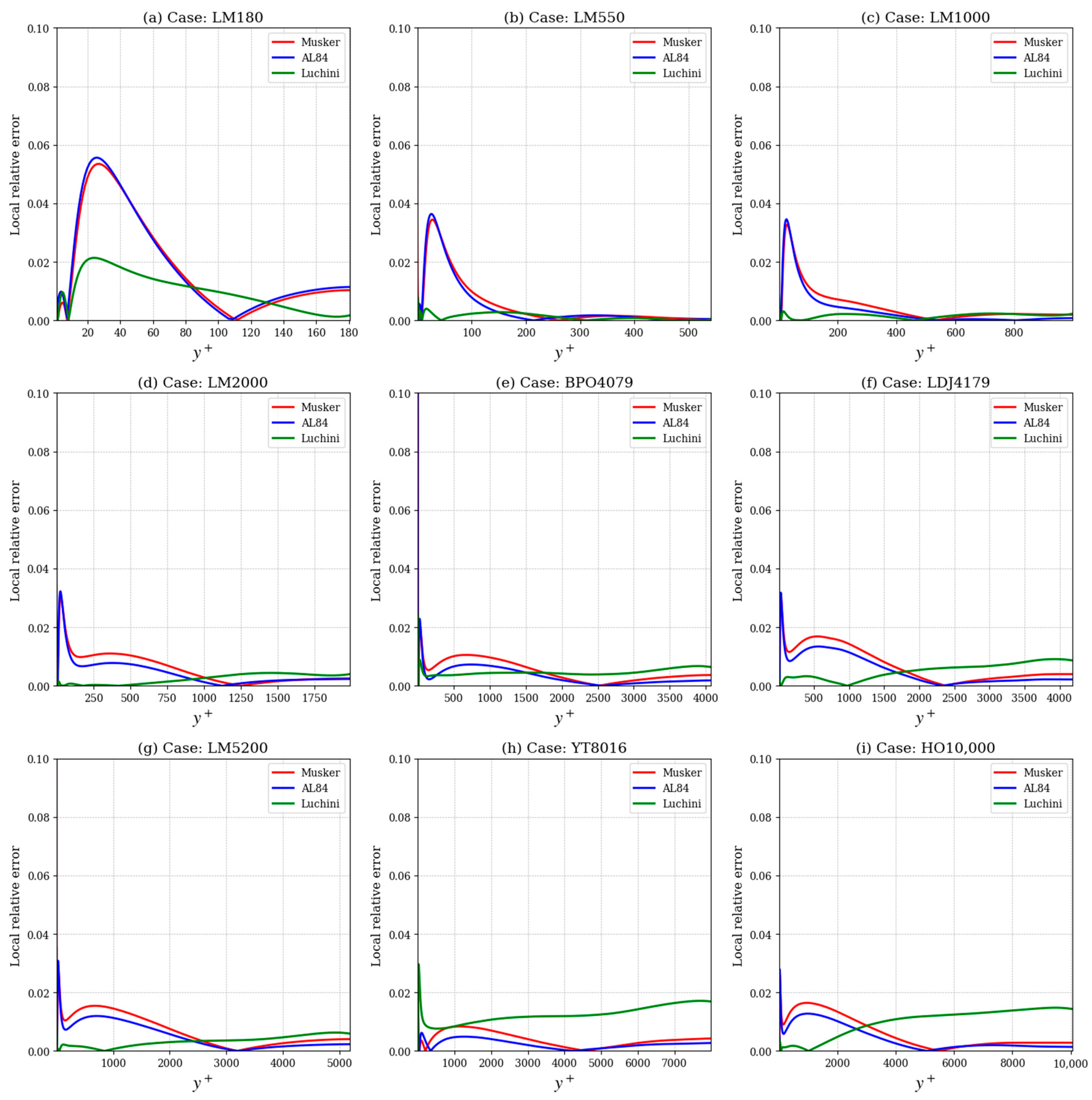
Profiles of Local Relative Error
3.2. Viscous and Reynolds Shear Stress Profiles
3.2.1. Viscous Stress Profiles
3.2.2. Relative Error in Profiles of Viscous Stress
3.2.3. Reynolds Shear Stress Profiles
3.2.4. Errors in Reynolds Shear Stress Profiles
4. Discussion and Conclusions
Author Contributions
Funding
Data Availability Statement
Conflicts of Interest
References
- Dixit, S.A.; Gupta, A.; Choudhary, H.; Prabhakaran, T. Generalized scaling and model for friction in wall turbulence. Phys. Rev. Lett. 2024, 132, 014001. [Google Scholar] [CrossRef]
- Lyu, S.; Kou, J.; Adams, N.A. Machine-learning-augmented domain decomposition method for near-wall turbulence modeling. Phys. Rev. Fluids 2024, 9, 044603. [Google Scholar] [CrossRef]
- Benjamin, M.; Domino, S.P.; Iaccarino, G. Neural networks for large eddy simulations of wall-bounded turbulence: Numerical experiments and challenges. Eur. Phys. J. E 2023, 46, 55. [Google Scholar] [CrossRef]
- Abdelaziz, M.; Djenidi, L.; Ghayesh, M.H.; Chin, R. On predictive models for the equivalent sand grain roughness for wall-bounded turbulent flows. Phys. Fluids 2024, 36, 015125. [Google Scholar] [CrossRef]
- Bao, T.; Hu, J.; Huang, C.; Yu, Y. Smoothed particle hydrodynamics with κ-ε closure for simulating wall-bounded turbulent flows at medium and high Reynolds numbers. Phys. Fluids 2023, 35, 085114. [Google Scholar] [CrossRef]
- Pirozzoli, S.; Smits, A.J. Outer-layer universality of the mean velocity profile in turbulent wall-bounded flows. Phys. Rev. Fluids 2023, 8, 064607. [Google Scholar] [CrossRef]
- Deshpande, R.; Zampiron, A.; Chandran, D.; Smits, A.J.; Marusic, I. Near-Wall Flow Statistics in High-Reτ Drag-Reduced Turbulent Boundary Layers. Flow Turbul. Combust. 2024, 113, 3–25. [Google Scholar] [CrossRef]
- Cremades, A.; Hoyas, S.; Deshpande, R.; Quintero, P.; Lellep, M.; Lee, W.J.; Monty, J.P.; Hutchins, N.; Linkmann, M.; Marusic, I.; et al. Identifying regions of importance in wall-bounded turbulence through explainable deep learning. Nat. Commun. 2024, 15, 3864. [Google Scholar] [CrossRef] [PubMed]
- Ahmad, T.; Zhang, D. A critical review of comparative global historical energy consumption and future demand: The story told so Far. Energy Rep. 2020, 6, 1973–1991. [Google Scholar] [CrossRef]
- Rothenberg, G. A Realistic look at CO2 emissions, climate change and the role of sustainable chemistry. Sustain. Chem. Clim. Action 2023, 2, 100012. [Google Scholar] [CrossRef]
- Ricco, P.; Skote, M.; Leschziner, M.A. A review of turbulent skin-friction drag reduction by near-wall transverse forcing. Prog. Aerosp. Sci. 2021, 123, 100713. [Google Scholar] [CrossRef]
- Andrade, D.M.; De Freitas Rachid, F.B.; Tijsseling, A.S. A new model for fluid transients in piping systems taking into account the fluid–structure interaction. J. Fluids Struct. 2022, 114, 103720. [Google Scholar] [CrossRef]
- Jing, J.; Guo, Y.; Karimov, R.; Sun, J.; Huang, W.; Chen, Y.; Shan, Y. Drag Reduction Related to Boundary Layer Control in Transportation of Heavy Crude Oil by Pipeline: A Review. Ind. Eng. Chem. Res. 2023, 62, 14818–14834. [Google Scholar] [CrossRef]
- Foggi Rota, G.; Monti, A.; Rosti, M.E.; Quadrio, M. Saving energy in turbulent flows with unsteady pumping. Sci. Rep. 2023, 13, 1299. [Google Scholar] [CrossRef]
- Giahi, M.; Bergstrom, D.J.; Singh, B. Computational fluid dynamics analysis of an agricultural spray in a crossflow. Biosyst. Eng. 2023, 230, 329–343. [Google Scholar] [CrossRef]
- Payri, R.; Gimeno, J.; Martí-Aldaraví, P.; Martínez, M. Transient nozzle flow analysis and near field characterization of gasoline direct fuel injector using Large Eddy Simulation. Int. J. Multiph. Flow 2022, 148, 103920. [Google Scholar] [CrossRef]
- Li, F.; Wang, Z.; Lee, C.; Ma, F.; Yang, W. Visualization and simulation study on impacts of wall roughness on spray characteristics of ducted fuel injection. Appl. Therm. Eng. 2022, 211, 118380. [Google Scholar] [CrossRef]
- Sosnowski, T.R.; Florkiewicz, E.; Sosnowski, K. Use of process intensification concepts for targeted delivery of inhaled aerosolized medicines. Chem. Eng. Process.-Process Intensif. 2024, 203, 109902. [Google Scholar] [CrossRef]
- Kuprat, A.P.; Feng, Y.; Corley, R.A.; Darquenne, C. Subject-specific multi-scale modeling of the fate of inhaled aerosols. J. Aerosol Sci. 2025, 183, 106471. [Google Scholar] [CrossRef] [PubMed]
- Fogliatto, E.; Clifford, I. Assessment of wall models for coarse-mesh RANS simulations. Ann. Nucl. Energy 2024, 209, 110807. [Google Scholar] [CrossRef]
- Serra, N. Revisiting RANS turbulence modelling used in built-environment CFD simulations. Build. Environ. 2023, 237, 110333. [Google Scholar] [CrossRef]
- Jiménez, J. A Perron–Frobenius analysis of wall-bounded turbulence. J. Fluid Mech. 2023, 968, A10. [Google Scholar] [CrossRef]
- Pirozzoli, S.; Orlandi, P. Natural grid stretching for DNS of wall-bounded flows. J. Comput. Phys. 2021, 439, 110408. [Google Scholar] [CrossRef]
- Khan, H.H.; Anwer, S.F.; Hasan, N.; Sanghi, S. Development and optimisation of a DNS solver using open-source library for high-performance computing. Int. J. Comput. Fluid Dyn. 2021, 35, 433–450. [Google Scholar] [CrossRef]
- Idelsohn, S.R.; Gimenez, J.M.; Larreteguy, A.E.; Nigro, N.M.; Sívori, F.M.; Oñate, E. The P-DNS method for turbulent fluid flows: An overview. Arch. Comput. Methods Eng. 2024, 31, 973–1021. [Google Scholar] [CrossRef]
- Kim, J.; Moin, P.; Moser, R. Turbulence statistics in fully developed channel flow at low Reynolds number. J. Fluid Mech. 1987, 177, 133–166. [Google Scholar] [CrossRef]
- Hoyas, S.; Oberlack, M.; Alcántara-Ávila, F.; Kraheberger, S.V.; Laux, J. Wall turbulence at high friction Reynolds numbers. Phys. Rev. Fluids 2022, 7, 014602. [Google Scholar] [CrossRef]
- Musker, A.J. Explicit expression for the smooth wall velocity distribution in a turbulent boundary layer. AIAA J. 1979, 17, 655–657. [Google Scholar] [CrossRef]
- Liakopoulos, A. Explicit representations of the complete velocity profile in a turbulent boundary layer. AIAA J. 1984, 22, 844–846. [Google Scholar] [CrossRef]
- Luchini, P. Universality of the turbulent velocity profile. Phys. Rev. Lett. 2017, 118, 224501. [Google Scholar] [CrossRef]
- Luchini, P. The open channel in a uniform representation of the turbulent velocity profile across all parallel geometries. J. Fluid Mech. 2024, 979, R1. [Google Scholar] [CrossRef]
- Workshop “Outstanding Challenges in Wall Turbulence and Lessons to be Learned from Pipes”, KAUST, Riyadh. 26–28 February 2024. Available online: https://turbulenceworkshop.kaust.edu.sa (accessed on 1 January 2025).
- Marusic, I.; McKeon, B.J.; Monkewitz, P.A.; Nagib, H.M.; Smits, A.J.; Sreenivasan, K.R. Wall-bounded turbulent flows at high Reynolds numbers: Recent advances and key issues. Phys. Fluids 2010, 22, 065103. [Google Scholar] [CrossRef]
- Jiménez, J. Near-wall turbulence. Phys. Fluids 2013, 25, 101302. [Google Scholar] [CrossRef]
- De Maio, M.; Latini, B.; Nasuti, F.; Pirozzoli, S. Direct numerical simulation of turbulent flow in pipes with realistic large roughness at the wall. J. Fluid Mech. 2023, 974, A40. [Google Scholar] [CrossRef]
- Heinz, S. On mean flow universality of turbulent wall flows. I. High Reynolds number flow analysis. J. Turbul. 2018, 19, 929–958. [Google Scholar] [CrossRef]
- Heinz, S. On mean flow universality of turbulent wall flows. II. Asymptotic flow analysis. J. Turbul. 2019, 20, 174–193. [Google Scholar] [CrossRef]
- Heinz, S. The asymptotic structure of canonical wall-bounded turbulent flows. Fluids 2024, 9, 25. [Google Scholar] [CrossRef]
- Heinz, S. The Law of the Wall and von Kármán Constant: An Ongoing Controversial Debate. Fluids 2024, 9, 63. [Google Scholar] [CrossRef]
- Liakopoulos, A. Fluid Mechanics, 2nd ed.; Tziolas Publications: Thessaloniki, Greece, 2019; ISBN 978-960-418-774-4. (In Greek) [Google Scholar]
- Landau, L.D.; Lifshitz, E.M. Fluid Mechanics: Course of Theoretical Physics, Volume 6, 2nd ed.; Pergamon Press: Oxford, UK, 1987; ISBN 0-08-033933-6. [Google Scholar]
- Coles, D. The law of the wake in the turbulent boundary layer. J. Fluid Mech. 1956, 1, 191–226. [Google Scholar] [CrossRef]
- Pope, S.B. Turbulent Flows, 1st ed.; Cambridge University Press: Cambridge, UK; New York, NY, USA, 2000; ISBN 978-0521598866. [Google Scholar]
- Granville, P.S. Similarity-Law Characterization Methods for Arbitrary Hydrodynamic Roughnesses; Bethesda: Rockville, MD, USA, 1978; Available online: https://apps.dtic.mil/sti/citations/ADA053563 (accessed on 1 September 2023).
- Wolfram|Alpha. Available online: https://www.wolframalpha.com (accessed on 17 February 2025).
- Palasis, A. Turbulent Boundary Layers: Analysis of DNS Data. Diploma Thesis, Department of Civil Engineering, University of Thessaly, Volos, Greece, 31 August 2021. (In Greek). [Google Scholar]
- Liakopoulos, A.; Palasis, A. On the Composite Velocity Profile in Zero Pressure Gradient Turbulent Boundary Layer: Comparison with DNS Datasets. Fluids 2023, 8, 260. [Google Scholar] [CrossRef]
- Liakopoulos, A.; Palasis, A. Turbulent Channel Flow: Direct Numerical Simulation-Data-Driven Modeling. Fluids 2024, 9, 62. [Google Scholar] [CrossRef]
- Lee, M.; Moser, R.D. Direct numerical simulation of turbulent channel flow up to Reτ = 5200. J. Fluid Mech. 2015, 774, 395–415. [Google Scholar] [CrossRef]
- Bernardini, M.; Pirozzoli, S.; Orlandi, P. Velocity statistics in turbulent channel flow up to Reτ = 4000. J. Fluid Mech. 2014, 742, 171–191. [Google Scholar] [CrossRef]
- Lozano-Durán, A.; Jiménez, J. Effect of the computational domain on direct simulations of turbulent channels up to Reτ = 4200. Phys. Fluids 2014, 26, 011702. [Google Scholar] [CrossRef]
- Yamamoto, Y.; Tsuji, Y. Numerical evidence of logarithmic regions in channel flow at Reτ = 8000. Phys. Rev. Fluids 2018, 3, 012602. [Google Scholar] [CrossRef]
- Zhu, C.; Byrd, R.H.; Lu, P.; Nocedal, J. Algorithm 778: L-BFGS-B: Fortran subroutines for large-scale bound-constrained optimization. ACM Trans. Math. Softw. (TOMS) 1997, 23, 550–560. [Google Scholar] [CrossRef]
- Byrd, R.H.; Lu, P.; Nocedal, J.; Zhu, C. A limited memory algorithm for bound constrained optimization. SIAM J. Sci. Comput. 1995, 16, 1190–1208. [Google Scholar] [CrossRef]
- Landahl, M.T.; Mollo-Christensen, E. Turbulence and Random Processes in Fluid Mechanics, 2nd ed.; Cambridge University Press: Cambridge, New York, 1992; ISBN 978-0521422130. [Google Scholar]
- Luchini, P. Structure and interpolation of the turbulent velocity profile in parallel flow. Eur. J. Mech. -B/Fluids 2018, 71, 15–34. [Google Scholar] [CrossRef]
- Liakopoulos, A. Computation of high speed turbulent boundary-layer flows using the k–ϵ turbulence model. Int. J. Numer. Methods Fluids 1985, 5, 81–97. [Google Scholar] [CrossRef]
- Sofos, F.; Chatzoglou, E.; Liakopoulos, A. An assessment of SPH simulations of sudden expansion/contraction 3-D channel flows. Comput. Part. Mech. 2022, 9, 101–115. [Google Scholar] [CrossRef]
- Sahan, R.A.; Albin, D.C.; Sahan, N.K.; Liakopoulos, A. Artificial neural network-based low-order dynamical modeling and intelligent control of transitional flow systems. In Proceedings of the Sixth IEEE Conference on Control Applications, Hartford, CT, USA, 5–7 October 1997. [Google Scholar]


| Case | Datasets | |
|---|---|---|
| LM180 | Lee and Moser, 2015 [49] | 182 |
| LM550 | Lee and Moser, 2015 [49] | 544 |
| LM1000 | Lee and Moser, 2015 [49] | 1000 |
| LM2000 | Lee and Moser, 2015 [49] | 1995 |
| BPO4079 | Bernardini, Pirozzoli and Orlandi, 2014 [50] | 4079 |
| LDJ4179 | Lozano-Durán and Jiménez, 2014 [51] | 4179 |
| LM5200 | Lee and Moser, 2015 [49] | 5186 |
| YT8016 | Yamamoto and Tsuji, 2018 [52] | 8016 |
| HO10,000 | Hoyas, Oberlack et al., 2022 [27] | 10,049 |
| Case | (Musker) | (AL84) | |||
|---|---|---|---|---|---|
| LM180 | 182 | 0.41 | 5.0 | 0.16 | 0.15 |
| LM550 | 544 | 0.41 | 5.0 | 0.14 | 0.12 |
| LM1000 | 1000 | 0.41 | 5.0 | 0.17 | 0.14 |
| LM2000 | 1995 | 0.41 | 5.0 | 0.20 | 0.18 |
| BPO4079 | 4079 | 0.41 | 5.0 | 0.17 | 0.14 |
| LDJ4179 | 4179 | 0.41 | 5.0 | 0.16 | 0.13 |
| LM5200 | 5186 | 0.41 | 5.0 | 0.18 | 0.15 |
| YT8016 | 8016 | 0.41 | 5.0 | 0.13 | 0.10 |
| HO10,000 | 10,049 | 0.41 | 5.0 | 0.14 | 0.11 |
| Case | Model | |||
|---|---|---|---|---|
| LM180 | 182 | Musker | 0.3535 | 0.9965 |
| LM550 | 544 | Musker | 0.1765 | 0.9991 |
| LM1000 | 1000 | Musker | 0.1603 | 0.9992 |
| LM2000 | 1995 | Musker | 0.1691 | 0.9991 |
| BPO4079 | 4079 | Musker | 0.1441 | 0.9993 |
| LDJ4179 | 4179 | Musker | 0.2121 | 0.9976 |
| LM5200 | 5186 | Musker | 0.2127 | 0.9980 |
| YT8016 | 8016 | Musker | 0.1162 | 0.9992 |
| HO10,000 | 10,049 | Musker | 0.2047 | 0.9974 |
| LM180 | 182 | AL84 | 0.3627 | 0.9963 |
| LM550 | 544 | AL84 | 0.1766 | 0.9991 |
| LM1000 | 1000 | AL84 | 0.1518 | 0.9993 |
| LM2000 | 1995 | AL84 | 0.1441 | 0.9994 |
| BPO4079 | 4079 | AL84 | 0.1066 | 0.9996 |
| LDJ4179 | 4179 | AL84 | 0.1711 | 0.9984 |
| LM5200 | 5186 | AL84 | 0.1699 | 0.9987 |
| YT8016 | 8016 | AL84 | 0.0703 | 0.9997 |
| HO10,000 | 10,049 | AL84 | 0.1557 | 0.9985 |
| LM180 | 182 | Luchini | 0.1663 | 0.9992 |
| LM550 | 544 | Luchini | 0.0266 | 1.0000 |
| LM1000 | 1000 | Luchini | 0.0309 | 1.0000 |
| LM2000 | 1995 | Luchini | 0.0552 | 0.9999 |
| BPO4079 | 4079 | Luchini | 0.1023 | 0.9996 |
| LDJ4179 | 4179 | Luchini | 0.1287 | 0.9991 |
| LM5200 | 5186 | Luchini | 0.0813 | 0.9997 |
| YT8016 | 8016 | Luchini | 0.2799 | 0.9954 |
| HO10,000 | 10,049 | Luchini | 0.2681 | 0.9956 |
| Musker | AL84 | Luchini | |
|---|---|---|---|
| 182 | |||
| 544 | |||
| 1000 | |||
| 1995 | |||
| 4079 | |||
| 5186 | |||
| 8016 | |||
| 10,049 | |||
| Musker | AL84 | Luchini | by DNS | ||
|---|---|---|---|---|---|
| 182 | 180.6 | 7.01 | 8.22 | 1.59 | 6.40 |
| 544 | 541.2 | 9.53 | 1.17 | 6.33 | 1.31 |
| 1000 | 997.4 | 4.03 | 4.93 | 3.65 | 5.38 |
| 1995 | 1990.6 | 1.33 | 1.79 | 1.95 | 1.68 |
| 5186 | 5180.7 | 1.61 | 3.27 | 7.99 | 2.91 |
| 8016 | 7996.0 | 3.89 | 4.77 | 4.67 | 7.76 |
| 10,049 | 10049.3 | 8.98 | 5.98 | 4.38 | 0 |
Disclaimer/Publisher’s Note: The statements, opinions and data contained in all publications are solely those of the individual author(s) and contributor(s) and not of MDPI and/or the editor(s). MDPI and/or the editor(s) disclaim responsibility for any injury to people or property resulting from any ideas, methods, instructions or products referred to in the content. |
© 2025 by the authors. Licensee MDPI, Basel, Switzerland. This article is an open access article distributed under the terms and conditions of the Creative Commons Attribution (CC BY) license (https://creativecommons.org/licenses/by/4.0/).
Share and Cite
Palasis, A.; Liakopoulos, A.; Sofiadis, G. From Direct Numerical Simulations to Data-Driven Models: Insights into Mean Velocity Profiles and Turbulent Stresses in Channel Flows. Modelling 2025, 6, 18. https://doi.org/10.3390/modelling6010018
Palasis A, Liakopoulos A, Sofiadis G. From Direct Numerical Simulations to Data-Driven Models: Insights into Mean Velocity Profiles and Turbulent Stresses in Channel Flows. Modelling. 2025; 6(1):18. https://doi.org/10.3390/modelling6010018
Chicago/Turabian StylePalasis, Apostolos, Antonios Liakopoulos, and George Sofiadis. 2025. "From Direct Numerical Simulations to Data-Driven Models: Insights into Mean Velocity Profiles and Turbulent Stresses in Channel Flows" Modelling 6, no. 1: 18. https://doi.org/10.3390/modelling6010018
APA StylePalasis, A., Liakopoulos, A., & Sofiadis, G. (2025). From Direct Numerical Simulations to Data-Driven Models: Insights into Mean Velocity Profiles and Turbulent Stresses in Channel Flows. Modelling, 6(1), 18. https://doi.org/10.3390/modelling6010018