Abstract
Solid–liquid phase transitions of metals and alloys play an important role in many technical processes. Therefore, corresponding numerical process simulations need adequate models. The enthalpy method is the current state-of-the-art approach for this task. However, this method has some limitations regarding multicomponent alloys as it does not consider the enthalpy of mixing, for example. In this work, we present a novel CALPHAD-informed version of the enthalpy method that removes these drawbacks. In addition, special attention is given to the handling of polymorphic as well as solid–liquid phase transitions. Efficient and robust algorithms for the conversion between enthalpy and temperature were developed. We demonstrate the capabilities of the presented method using two different implementations: a lattice Boltzmann and a finite difference solver. We proof the correct behaviour of the developed method by different validation scenarios. Finally, the model is applied to electron beam powder bed fusion—a modern additive manufacturing process for metals and alloys that allows for different powder mixtures to be alloyed in situ to produce complex engineering parts. We reveal that the enthalpy of mixing has a significant effect on the temperature and lifetime of the melt pool and thus on the part properties.
1. Introduction
In numerical simulations, a suitable modelling of the material behaviour is required to make good predictions about physical processes. This becomes even more important when multicomponent alloys are considered. They are needed in engineering applications to meet increasingly difficult requirements in the form of, e.g., mechanical load, high temperatures and corrosive environments. However, the necessary material parameters are often difficult to determine or inaccessible in the current literature—especially if it comes to modelling the concentration dependence of the material behaviour of multicomponent systems.
For that purpose, the CALPHAD (CALculation of PHAse Diagrams) method can provide a remedy [1,2,3]. Its core idea is to model the Gibbs energy G of each phase using suitable functions with adjustable parameters and finding the equilibrium properties by minimising the total Gibbs energy [4]. In doing so, the fit parameters are determined using, e.g., experimental data or results from first-principles calculations and are saved in databases for the corresponding alloy systems [5]. Using this approach, the thermodynamic properties of higher-order multicomponent alloys can be described by extrapolation from known binary systems [6,7]. These thermodynamic datasets, in turn, allow for the calculation of the temperature and concentration dependence of various material parameters, which can be used in numerical simulations.
In the realm of phase-field simulations, the coupling with CALPHAD calculations has been proven to be beneficial [8,9] and is already well-established [10,11,12]. It is based on the concept of local equilibrium, which enables the possibility to employ equilibrium thermodynamic data even though non-equilibrium processes are simulated [12]. In practice, for the chemical free energy function in the phase-field model, a CALPHAD-type description can be used, which is accordingly filled with information from a suitable CALPHAD database [10]. Possible applications are the simulation of Ostwald ripening, spinodal decomposition or dendritic solidification [8,13,14].
For other simulation techniques like the enthalpy method [15], this coupling is not as straightforward and will be addressed in this work. In many simulations of physical processes, this method is used to handle the moving solid–liquid phase boundaries during heat conduction problems. Its biggest advantage is that a single equation is sufficient to describe the heat flow in both phases as well as the phase boundary. In particular, no additional boundary conditions have to be fulfilled at the interface. This way, it is possible to employ a fixed grid for the numerical calculations [16].
Due to its convenience, the enthalpy method is widely applied in the field of solidification of metals and alloys [17,18] as well as welding and additive manufacturing simulations [19,20,21,22,23,24,25,26,27]. However, in these works, the enthalpy of mixing is not considered. Although often neglected, Collins et al. [28] have shown that an exothermic enthalpy of mixing can significantly reduce the necessary energy input for the in situ alloying of powder mixtures. Thus, simulation models of these processes require a thermodynamically refined version of the enthalpy method, in which the enthalpy of mixing is considered. The development of such a model is the main objective of the presented work. Another drawback of the conventional enthalpy method is the necessity to specify the input material parameters manually and individually. Often times [20,22,24,26], only linear approximations are used for the temperature and composition dependence of these parameters for lack of more detailed data.
Therefore, we present a novel variant of the enthalpy method that comes without the necessity to separately specify the latent heat of fusion. This is achieved by directly using the specific enthalpy and fluid fraction data from CALPHAD calculations to describe the solid–liquid phase transition. Further advantages are an inherent consideration of the enthalpy of mixing, with no additional simplification of the specific heat capacity as it is directly calculated from the input enthalpy–temperature relationship and an implicit consideration of the solidus and liquidus temperatures, so that phase diagrams do not have to be modelled separately. Special attention will be given to the handling of phase transitions.
As Küng et al. [26] and Chouhan et al. [29] have shown, the conventional way of coupling CALPHAD calculations with numerical simulations for metal processing is to provide processed data like phase diagrams. In this work, a novel method for directly using composition and temperature-dependent enthalpy surfaces stored in thermodynamic databases as an input to the enthalpy method to model the behaviour of alloy systems is presented. In the past, basic approaches for using enthalpy data from thermodynamic databases in combination with the enthalpy method have already been investigated to study certain alloys. Ohsasa et al. [30,31] used the CALPHAD method to calculate single temperature-dependent enthalpy curves for fixed alloy compositions as an input to an enthalpy method-based thermal solver to simulate the solidification process. They showed that the realistic thermodynamic data are crucial to accurately reproduce experimentally measured cooling curves. However, this method only works for fixed concentrations and therefore does not include the concentration dependencies necessary for simulations with varying compositions—especially regarding in situ alloying processes. Consequently, solidus and liquidus curves as well as the enthalpy of mixing effect are not considered. A similar approach was chosen by Saad et al. [32] which, albeit more sophisticated, still only applies to alloys with fixed compositions. To the best of the authors’ knowledge, until now there is no published model in the scientific literature that combines thermodynamic alloy data from CALPHAD calculations with the enthalpy method for simulations with varying concentrations. In particular, there is currently no published model for the simulation of in situ alloying during powder bed fusion additive manufacturing that considers the effect of the enthalpy of mixing.
In the next section, the standard enthalpy method as well as its conventional adaptation for multicomponent alloys will be recalled before the newly developed CALPHAD-informed version is explained. After that, the two utilized solvers are described. These are an in-house developed lattice Boltzmann-based simulation software and a finite difference solver, both written in C++. Finally, the model is applied to different simulation setups for verification purposes as well as a multi-material simulation of an in situ alloying process during electron beam powder bed fusion of an exemplary powder mixture.
2. Enthalpy Models
2.1. The Enthalpy Method
Due to their relevance for technical processes, solid–liquid phase transitions are of great interest to the scientific community and have been studied intensively in recent decades. In general, the underlying physics for a system without convection, for one dimension x and a pure substance with a distinct melting point , can be described by the three following equations [33]:
where T is the temperature, t the time, x the spatial coordinate, the position of the solid–liquid phase boundary, stands for the thermal diffusivity, for the thermal conductivity, for the density and L denotes the latent heat of fusion. The subscripts s and l indicate the solid and liquid phase, respectively. The third equation describes the boundary condition at the interface and can be derived from the requirement at the phase boundary [33]. This scenario has been rigorously studied as early as 1889 by Stefan [34], which led to the term Stefan problem.
Regarding numerical investigations, however, the moving phase boundary poses a demanding challenge for thermal solvers. In general, two different strategies have been developed to tackle this problem: variable domain formulations and the enthalpy method [16]. In the former approach, heat conduction is solved separately in the solid and the liquid phase using the Equations (1) and (2), so that the interface has to be tracked at all times, which also led to the term front tracking schemes [35]. Popular forms are, e.g., the variable time step method by Douglas and Gallie [36] or the moving grid method by Murray and Landis [37]. However, the enthalpy method, pioneered by Atthey [38], Shamsundar and Sparrow [15] as well as Meyer [39], has gained widespread acceptance due to its convenience as only one equation has to be solved for the entire geometry—including the phase boundary. In particular, it can be shown that the boundary condition at the interface is implicitly fulfilled and a boundary tracking is not necessary [16]. With that, the Equations (1)–(3) can be replaced by
where H is the enthalpy [33]. To solve this numerically, the enthalpy–temperature relationship has to be used to replace one of the two quantities. It is usually approximated by a piecewise defined linear function similar to
with the heat capacity [16,40].
2.2. Conventional Enthalpy Model for Multicomponent Systems
Equation (5) is generally valid for systems with a constant composition. To account for varying concentrations, the method has to be extended accordingly. The state-of-the-art approach for that is described in the following section using the implementation by Küng et al. [26], which we used to simulate powder bed fusion additive manufacturing processes until now. Similar models were also presented by Chouhan et al. [29] and Tang et al. [41].
In general, the specific enthalpy h is given by
where the function is bijective for a fixed composition . As in this work only binary alloys are considered, the composition is sufficiently described by a single mass fraction parameter . Typically, it is set to the alloying element B for an arbitrary alloy AB: . At the same time, one has using . The symbol stands for the specific heat capacity at constant pressure.
Under the assumption that is independent of the temperature inside the solid () and liquid phase () and with the simplification of an average specific heat capacity in the mushy zone, one has [26]
All material parameters on the right-hand side of Equation (7) are dependent on the composition. However, this is not denoted explicitly for the sake of better readability. The function is divided into three intervals, which are defined by the solidus () and liquidus temperature (), respectively. Additionally, in the mushy zone, the application of the latent heat is controlled by the fluid fraction . These quantities were modelled according to the phase diagram, which can be performed by approximating the solidus and liquidus curves by means of linear approximations between discrete data points. An example of this concept is depicted in Figure 1 using an arbitrary, fully miscible alloy system AB.

Figure 1.
Exemplary phase diagram for an arbitrary, fully miscible alloy system AB. The solidus and liquidus curves are approximated via linear interpolations between manually set data points, which are depicted using grey crosses. For an initial composition , the red lines represent the lever rule, which is used to determine the composition of the solid and liquid phase at a certain temperature inside the two-phase region.
Based on this, the fluid fraction can be calculated in dependence on the composition and temperature according to the lever rule [26]:
where the composition of the liquid and the solid phase are represented by and , respectively.
By means of this example, the drawbacks of the conventional enthalpy method for multicomponent alloy systems become apparent. Firstly, gross simplifications are applied to the enthalpy–temperature relationship by neglecting the enthalpy of mixing and assuming to be independent of the temperature. Secondly, the necessary input material parameters , L and / can be hard to find or inaccessible in the scientific literature. And lastly, the procedure of discretising the solidus and liquidus lines has to be performed again manually for every new material system. To resolve these issues, we developed a novel CALPHAD-based approach, which is presented in the following section.
2.3. The CALPHAD-Informed Enthalpy Method
For the sake of simplicity, the CALPHAD-informed enthalpy method is presented in this work using a binary alloy system. It can readily be extended to ternary alloys by appropriately adjusting the methods for the generation of the necessary CALPHAD data as well as the conversion algorithms presented in Section 2.3.2. However, the underlying simulation software itself also needs to be capable of handling ternary systems. This includes a description of the composition field by two independent compositional parameters and a second advection diffusion equation to consider all diffusion fluxes. In this context, it has to be noted that the method relies on the availability of appropriate thermodynamic data, especially for the solid–liquid phase transition. When applied to ternary (and higher-order) systems, additional interaction parameters may be necessary to accurately capture the material behaviour using the CALPHAD method. Thus, when addressing multicomponent systems, it is important to ensure the use of high-quality thermodynamic databases and to consider their limitations.
In the conventional enthalpy method, the specific enthalpy is calculated from heat capacity data, as described in Section 2.2. The fundamental idea of the CALPHAD-informed approach is to invert this calculation. Concretely, the specific enthalpy is calculated using thermodynamic databases and directly provided as a simulation input, from which the specific heat capacity is determined via
This offers the advantage of a significantly more realistic modelling of the enthalpy–temperature relation as no simplifications are made for the highly non-linear temperature-dependent progression of the specific heat capacity or latent heat. Thus, better results can be expected for the simulation of heat conduction and solid–liquid phase transition in metallic materials. The calculation of is necessary as it is used to obtain the thermal diffusivity, which is needed for thermal solvers, as indicated by Equation (14). Furthermore, also other physical models, e.g., for the calculation of evaporation phenomena, can be dependent on .
For highly optimised simulation programs, direct function calls to thermodynamic databases are unfeasible as they are very time-consuming and therefore would significantly increase the computing time. Instead, it is more practical to generate the required thermodynamic data in advance and read them in at the program start via look-up tables. This way, only fast search algorithms and interpolations for the temperature–enthalpy conversion need to be executed at runtime.
The concept of our CALPHAD-based approach is summarised in Figure 2 by means of the CuCr alloy system. The procedure starts with the generation of the CALPHAD data, which is explained in Section 2.3.1 in detail. These data consist of the specific enthalpy and fluid fraction, which are calculated for n different compositions in combination with m different temperatures in a way that the whole relevant parameter space for and T are covered. The results are saved in the form of matrices, which are fed into the simulation software and loaded into the material model.
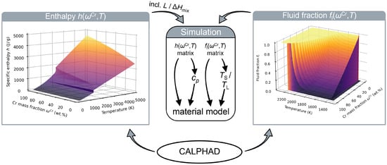
Figure 2.
Concept of the CALPHAD-informed material model for the CuCr alloy system. The necessary enthalpy h and fluid fraction data are calculated in dependence of the Cr mass fraction and temperature T using the CALPHAD method and fed into the simulation. This information is then used to determine further needed material parameters like the specific heat capacity or solidus and liquidus temperatures and .
The purpose of considering the fluid fraction data from CALPHAD calculations in addition to the specific enthalpy is to achieve a realistic modelling of the solid–liquid phase transition for moving phase boundaries. As can be seen in Figure 2, a linear approximation of the fluid fraction in the mushy zone would not reflect the material behaviour correctly. Typically, the fluid fraction is used to determine whether a certain cell or grid point is considered as solid or liquid for different simulation techniques. To avoid oscillating conversions, it is helpful to set the criterion for melting to , whereas for solidification has to be fulfilled [22].
Based on the jumps and the curvature of the enthalpy surface in Figure 2, it becomes apparent that the heat of fusion L and the enthalpy of mixing are already included in the enthalpy dataset by its very nature. Hence, the number of necessary input parameters and, accordingly, possible sources of error are reduced compared to the conventional enthalpy method. Another advantage of the presented model is the possibility to directly extract the solidus and liquidus temperature functions from the fluid fraction data, which can further reduce the number of input parameters that have to be specified manually. This becomes especially useful for complex alloy systems like AlCu, where the manual approximation of and is rather laborious [29].
2.3.1. Generation of the CALPHAD Data
For the generation of the necessary CALPHAD data, the software Thermo-Calc 2021b (Thermo-Calc Software AB, Solna, Sweden) [42] was used in combination with the material databases TCCU3 and TCTI2 for copper and titanium alloys, respectively. This was conducted by means of the Python interface for Thermo-Calc (TC-Python) in order to automatise and parallelise the calculations. The temperature and composition ranges as well as the corresponding increments used in this study are summarised in Table 1.

Table 1.
Overview of the used temperature and composition ranges combined with the corresponding increments for the specific enthalpy and fluid fraction data. The temperature range for should cover all occurring temperatures, while it can be reduced to the mushy zone for . Thus, different values are defined for the alloy systems CuCr and TiAl.
In doing so, it must be ensured that the chosen temperature range for the specific enthalpy covers all possibly occurring temperatures in the simulation. For the fluid fraction data, a reduced temperature section is sufficient as long as the solid–liquid phase transition is completely contained. At the same time, its temperature resolution has to be at least three times larger than the one used for the specific enthalpy which is important for the interpolation of the specific heat capacity in the mushy zone, explained in Section 2.3.3.
The actual calculations are performed using the batch equilibrium calculation module [43] in consideration of the prevalent process conditions. For example, for simulations of the electron beam powder bed fusion process [26], the pressure has to be adjusted to the technical vacuum atmosphere. Furthermore, the data for pure elements has to be calculated separately as all other elements have to be suspended for accurate results.
2.3.2. Numerical Implementation
The main issue regarding the implementation is the efficient handling of large datasets. While the heat conduction is calculated using the specific enthalpy, the current temperature is the common input and output quantity. Furthermore, it is often needed for other physical models inside a simulation software. Therefore, a bilateral conversion between enthalpy and temperature is required in every time step. Based on the typically long simulation times for physical processes, this conversion has to be implemented in an efficient and robust way. The easier case is the calculation of the specific enthalpy from given temperature and composition values , which is visualised in Figure 3.
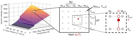
Figure 3.
Schematic illustration of the bilinear interpolation algorithm for the calculation of the specific enthalpy from a given () input data pair using the example of the CuCr system. The discrete values from CALPHAD calculations are depicted in grey. For an arbitrary () data pair (shown in red), the resulting specific enthalpy is calculated by bilinear interpolation between the neighbouring discrete values according to the present compositions and temperatures. In the first step, the neighbouring enthalpy data is interpolated with regard to the input composition (open red circles). These intermediate values are then interpolated to the specified temperature (filled red circle).
A section of the enthalpy data matrix is depicted using grey dots, where each dot represents a discrete data point. For an arbitrary input data pair (), the first step is to determine the neighbouring enthalpy data points. As the temperature and composition increments and are known, the exact row and column numbers of the neighbouring values can be calculated by and under consideration of the minimum temperature and concentration in the CALPHAD data. For example, using the values given in Table 1 and an exemplary temperature of 3000 K, the corresponding notional row number would be . This means that this input data point would be located between the 1166th and 1167th row. Using the hereby determined neighbouring values, the resulting specific enthalpy for the input data pair can be approximated by a bilinear interpolation between them [44].
In the reverse case , the specific enthalpy increments are not uniform due to the non-linear specific heat capacity of real alloy systems. This means that the position of the input enthalpy value inside the data matrix, which is necessary to calculate the corresponding temperature using the row numbers of the neighbouring h values, cannot be directly calculated like in the previously explained case . Thus, a suitable search algorithm had to be implemented. As this procedure has to be performed in every cell or grid point at every time step, it has to be highly efficient and robust. Therefore, an algorithm based on the interpolation search [45] was developed and adjusted to this application. A graphic representation for a fixed is shown in Figure 4.
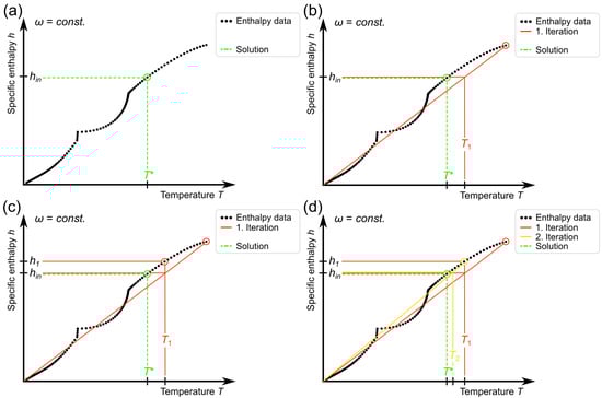
Figure 4.
Illustration of the procedure of the implemented search algorithm for the determination of the corresponding temperature to a specific enthalpy input value at a fixed composition. In every iteration, the method adjusts one of the two interval boundaries and determines the new approximation of the desired temperature value from a linear interpolation between the two boundaries. For clarity, stacked lines are drawn with a slight shift. (a) Depiction of the desired temperature for the input enthalpy . (b) First approximation based on the limits of the enthalpy data set. (c) Corresponding enthalpy value for the approximated temperature . (d) As , it is set as the new upper boundary for the next iteration, leading to the approximation .
The desired corresponding temperature value for the input enthalpy will be called in the following, as depicted in Figure 4a. For the first estimate , a linear interpolation between the lowest and highest values of the enthalpy data and is used, which is shown in Figure 4b. This is already a relatively good approximation for because the enthalpy curve does not deviate much from a straight line for the CuCr system. Next, as illustrated in Figure 4c, the corresponding enthalpy for the first iterative solution is determined. As in this case is above and due to the monotonically rising enthalpy curve, one can deduce that . Hence, is set as the new upper boundary, which narrows down the possible solutions. The next iteration, shown in Figure 4d, begins with a linear interpolation again; however, this time the boundary values are set to and . This scheme is continued until the boundaries do not change any more. Then, the two neighbouring temperature data points for are identified using a binary search method. Finally, a linear interpolation is performed in order to determine the exact corresponding temperature value for :
where and are the two neighbouring temperature values.
2.3.3. Handling of Phase Transitions
As described at the beginning of Section 2.3, the specific heat capacity can be calculated from the enthalpy data using Equation (9). Numerically, this can be performed with a simple central finite difference approach:
In doing so, the temperature difference should be chosen according to . In this work, a value of K was used.
Phase transitions can cause jumps in the enthalpy data due to the associated enthalpy of phase change, which leads to extremely high peaks in the specific heat capacity when it is calculated by differentiation. For the CuCr system, the specific enthalpy curve for and the resulting heat capacity data are shown in Figure 5a and Figure 5b, respectively.
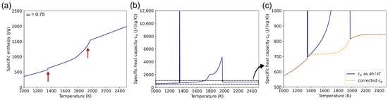
Figure 5.
(a) Enthalpy curve at a constant Cr mass fraction of 0.75 in the CuCr alloy system. Jumps due to the latent heat are marked with red arrows. (b) Specific heat capacity calculated from the enthalpy data in (a) using Equation (9). The large peaks originate from the marked enthalpy jumps. (c) Enlarged section of the diagram shown in (b) with an additional curve calculated using Equation (12), shown in orange.
As the enthalpy of phase change is already included in the specific enthalpy data and therefore considered in the simulation, the corresponding peaks have to be removed to prevent this effect from being introduced twice. Thus, for the mushy zone, a weighted specific heat capacity using at the solidus and liquidus temperature is introduced in order to eliminate these peaks:
With as the weighting factor, the corrected heat capacity curve is depicted in Figure 5c as the orange line. The small jump at the solidus temperature can be traced back to the fact that Cu and Cr are immiscible in the solid state. Therefore, upon reaching the melting temperature of Cu, the entire Cu fraction of the alloy melts all at once, which leads to an instant increase in the fluid fraction , as depicted in Figure 2.
Aside from the solid–liquid transition, polymorphic phase transitions can also be accompanied by a latent heat, which is demonstrated using the example of the TiAl alloy system in Figure 6. In Figure 6a, the specific enthalpy surface for TiAl, which was calculated using the CALPHAD method and the TCTI2 database, is depicted. Next to it, the corresponding specific heat capacity for the composition Ti-6Al is plotted. The data show two peaks, one owing to the solid–liquid phase transition and the other stemming from the allotropic phase transformation from -Ti to -Ti. In order to remove the latter, a filtering method has to be used, for example, based on a threshold value for a maximum allowed heat capacity.
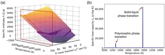
Figure 6.
(a) Specific enthalpy surface for the TiAl alloy system. The red rectangle marks a cutting plane for the composition Ti-6Al, in which the associated curve is highlighted using a dashed red line. (b) Corresponding specific heat capacity function for the composition highlighted in (a), showing two distinct peaks. The first one stems from the polymorphic phase transition from the to the phase, whereas the second one is related to the solid–liquid phase transition. The former peak is removed using a suitable filtering method.
3. Numerical Solvers
The presented CALPHAD-informed enthalpy method is applicable to any desired simulation technique. As an example, the implementation into a thermal lattice Boltzmann model in the form of the simulation software [46] and into a finite difference solver is discussed.
3.1. Simulation Software
The presented CALPHAD-based enthalpy model was devised to reform the material modelling of the in-house developed simulation software [46] in order to achieve a realistic prediction of the phenomena that occur during multi-material fabrication via electron beam powder bed fusion (PBF-EB). is a mesoscopic lattice Boltzmann-based simulation tool for the investigation of metallic powder bed fusion additive manufacturing processes, developed in C++. It focuses on the powder consolidation process, for which all necessary physical phenomena like heat conduction, phase transitions, fluid dynamics and evaporation are implemented. Details about the software and the manufacturing method can be found in previous publications [26,47]. The new material model constitutes a major improvement compared to the former one [26], as with the new method no simplifications are made for material parameters like the specific heat capacity or latent heat and the effect of the enthalpy of mixing is already considered in the underlying CALPHAD data.
In this software, the fluid dynamics is solved implicitly by the lattice Boltzmann (LB) method [48]. For the evolution of the thermal field, a separate LB model by Zhang et al. [49] is used, which was developed to solve general scalar balance equations. The underlying enthalpy conservation equation
considers two molecular fluxes: heat conduction and enthalpy diffusion (i.e., the effect of enthalpy being transported with a diffusion flux) [50]. The symbol represents the thermal conductivity, stands for the diffusion flux, for the velocity and for the density. In order to solve Equation (13) by the Zhang model, the temperature gradient has to be replaced by the enthalpy gradient. After this conversion and insertion of for , we obtain [26]
where D stands for the diffusion coefficient, for the thermal diffusivity and represents the thermal source term. This is where the novel CALPHAD-informed methodology comes into play. The specific enthalpy data, which are calculated using the CALPHAD method, act as an input to this equation. Furthermore, the transport coefficients and D are different in the solid and liquid phase, for which the transition is modelled by the CALPHAD-based fluid fraction. Another important scalar field quantity is the composition. To describe its evolution, the diffusion flux is calculated using finite differences and it is further advected based on the velocity field by a passive scalar transport model from Osmanlic et al. [51].
3.2. Finite Difference (FD) Solver
In order to show that the CALPHAD-informed enthalpy method is also applicable to other simulation techniques and to provide a comparison for the verification of the implementation into , the new model was coupled with a FD solver for the enthalpy balance equation. For that, Equation (13) was used as the foundation. As only the molecular fluxes were of interest, the velocity was set to zero:
To simplify the method further, a constant thermal conductivity was assumed. With the volume-specific enthalpy , one has
In addition, the two derivatives and can be evaluated together. For one dimension, the finite difference expression is [26]
where the subscripts denote a spatial discretisation with the grid point distance . The most important difference compared to the previously described thermal lattice Boltzmann model is that the first term on the right-hand side of Equation (16) does not have to be converted into an enthalpy description, so that this equation can be directly discretised and solved numerically. To do so, the FTCS (Forward Time Centred Space) scheme [52] was used, where the additional temporal discretisation is represented by superscripts using the time step . For one dimension and assuming a constant diffusion coefficient D, this reads
Based on this equation, the volume-specific enthalpy in the next time step can be calculated from the previous one by
The enthalpy diffusion term in Equation (16) only comes into effect when diffusion fluxes are present. To calculate the evolution of the composition field, the solution of the diffusion equation known as Fick’s second law
is similarly approximated by a finite difference approach. For a constant diffusion coefficient D, the one-dimensional formulation is
4. Verification Simulations
4.1. Diffusion Couple
With the first simulation setup, the consideration of the enthalpy of mixing as well as the conservation of enthalpy ought to be verified. It consisted of a diffusion couple with a Cu-rich () next to a Cr-rich () region, which are surrounded by periodic boundary conditions as depicted in Figure 7a. With as the numerical solver, diffusion was calculated between these two regions until the composition was constant everywhere at . The simulation domain was composed of a square lattice with a length of 100 cells. Using a cell size of 2 µm and a time step of ns, the relative diffusion length
was set to . This way, a simulated time of 10,000 time steps () was sufficient to reach the equilibrium state. Furthermore, the initial temperature was set to 2500 K, so that the whole domain remained liquid throughout the process. Thus, the results were not influenced by a phase transition. For the one-dimensional FD solver, all parameters were chosen equally.
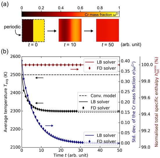
Figure 7.
(a) Depiction of the evolution of the simulation setup containing a diffusion couple with an initial Cu-rich () next to a Cr-rich () region, surrounded by periodic boundary conditions. At the end of the simulation, the composition field was constant at . (b) Diagram of the average temperature , the standard deviation of the Cr mass fraction and the normalised total specific enthalpy along the diffusion process for the lattice Boltzmann (LB) and finite difference (FD) solver using the CALPHAD-informed enthalpy method. The positive enthalpy of mixing in the CuCr alloy system results in a decrease in temperature of about 200 K. In contrast, the dashed black line shows the temperature progression using a conventional enthalpy method, which does not consider the enthalpy of mixing. Thus, the temperature stays constant throughout the simulation in this case.
In Figure 7b, the diagram shows the evolution of the average temperature , the standard deviation in the Cr mass fraction and the normalised total specific enthalpy along the diffusion process in black, blue and red, respectively. Both solvers show a very good agreement. By means of the curve, it is visible that the system indeed reaches a state of uniform composition. At the same time, remains constant at 100%, which confirms that the enthalpy conservation law is fulfilled. However, the data depicted in black illustrate that the temperature decreases from 2500 K to about 2300 K in the course of the diffusion process. This is a direct result of the enthalpy of mixing, which is included in the CALPHAD data. Hence, this effect does not have to be modelled separately, but is implicitly considered by applying the specific enthalpy data from CALPHAD calculations. For comparison, the dashed black curve depicts the temperature progression for the same simulation setup using the conventional enthalpy method. The fact that the temperature stays constant in this case confirms that the enthalpy of mixing has to be externally provided using appropriate thermodynamic data, for which the presented CALPHAD-informed enthalpy method provides a suitable approach.
To verify the plausibility of this relatively high decrease in temperature, the corresponding enthalpy of mixing was calculated and compared to data from the literature. With a specific heat capacity for CuCr50 in the liquid state of about 630 [53], one obtains an integral enthalpy of mixing of
This is in the same order of magnitude compared to the experimental results from Turchanin et al. [54,55], who report a value of about at a temperature of 1873 K. The difference between these two enthalpy values can essentially be traced back to the different starting temperatures as exhibits a certain temperature dependence. Nevertheless, the observed temperature decrease of about 200 K can be validated as reasonable by means of this comparison. Additionally, this experiment shows that the conversion algorithms between enthalpy and temperature described in Section 2.3.2 function properly as these calculations are performed repeatedly throughout the simulation without producing outliers or showing an accumulation of errors.
4.2. Coupled Transport Phenomena
The implementation of the thermal lattice Boltzmann model was further verified with respect to the coupled molecular transport phenomena of diffusion and heat conduction by comparing the simulation results between the LB and FD solvers. If both are in good agreement, a correct implementation can be expected. The setup consisted of a one-dimensional domain with a length of µm, for which a step-like composition distribution superimposed by a Gaussian temperature distribution is initially defined. The corresponding functions are described by
where and stand for the minimum and maximum temperature. The defined standard deviation as well as further material and simulation parameters are summarised in Table 2.
Table 2.
Summary of the used material and simulation parameters in the coupled transport phenomena simulation setup.
In order to achieve significant changes in the temperature and composition field, the simulated time was set to 20 ms. Furthermore, periodic boundary conditions were used to prevent unwanted boundary-related influences.
In Figure 8, the results after a simulated time of 10 ms and 20 ms are depicted together with the initial state. In general, an excellent agreement between the solutions from the LB and the FD solver can be seen. Thus, the numerical implementation of the thermal LB model is expected to be correct and the results concerning the molecular transport fluxes can be trusted. Moreover, it is confirmed that CALPHAD-informed enthalpy method can be applied to different solvers.
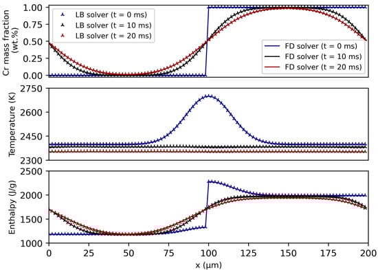
Figure 8.
Comparison of the results from the lattice Boltzmann (LB) and finite difference (FD) solver for a coupled heat conduction and diffusion problem. The material was modelled according to the presented CALPHAD-based method and the conversion between enthalpy and temperature was calculated using the algorithms in Section 2.3.2. An excellent agreement can be seen for the evolution of the composition, temperature and specific enthalpy distribution. The influence of the CALPHAD data is manifested in the enthalpy of mixing-induced decrease in temperature as well as in the asymmetric enthalpy field.
Regarding the composition distribution, a distinct smoothing of the step function towards a sinusoidal curve occurs as expected by the diffusion theory. As early as 10 ms into the simulation, the temperature distribution is completely homogenised because heat conduction is a significantly faster process than diffusion. At the same time, the average temperature decreases successively due to the positive enthalpy of mixing of the CuCr system. These two processes influence the resulting enthalpy distribution, whose asymmetry can be traced back to the asymmetric enthalpy–temperature relation that is contained in the CALPHAD data.
4.3. Stefan Problem
Finally, the correct handling of the solid–liquid phase transition was verified by means of the one-dimensional Stefan problem [34], which is normalised by a moving phase boundary that emerges from a constant-temperature heat source as depicted in Figure 9a. At first, a simplified setup with constant material parameters was chosen, so that the numerical results could be compared with the corresponding analytical solutions. The boundary conditions for the temperature distribution and in particular the phase boundary were given by
where was set to an arbitrary melting point of 1500 K for the whole domain of length l and was held constant at 3000 K. The other necessary material parameters were specified as kg/m3, J/kg and J/(kg K). This was achieved by creating simplified, arbitrary versions of the enthalpy and fluid fraction input files, in which the data values were adjusted to obtain said material parameters. Additionally, the thermal conductivity was set to 10 W/(m K), 50 W/(m K) and 100 W/(m K) in the three different scenarios. As a result, the thermal diffusivity with
had constant values of 4 mm2/s, 20 mm2/s and 40 mm2/s. With these simplifications, the one-dimensional Stefan problem can be solved analytically. The position of the solid–liquid phase boundary is given by [56,57]
where the factor is the solution of the transcendental equation
Using the previously stated parameters, one has . As only the positive value makes sense physically, the analytical solutions are uniquely determined. Their graphical representations are depicted in Figure 9a alongside the corresponding numerical data, which were obtained using the lattice Boltzmann-based thermal solver in . In doing so, the position of the solid–liquid interface was defined as the left-most cell, in which the fluid fraction is below 0.5.
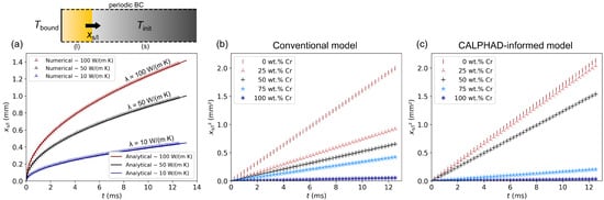
Figure 9.
Simulation of the Stefan problem for the analysis of the transient solid–liquid phase transition. (a) Simulation domain consisting of a rectangular bar with an initial temperature and a boundary condition with a constant value of 3000 K. The orange region depicts the already molten material. Below: Progression of the phase boundary over time for a simplified setup with three different thermal conductivities and otherwise constant material parameters. The numerical results are in excellent agreement with the analytical solutions. (b) Squared melt front position over time for five different compositions of the CuCr alloy system, calculated using a conventional enthalpy method. As expected, an increasing Cr content leads to a decrease in the melt front velocity due to a reduced thermal diffusivity. (c) Results from the same simulation setup calculated using the presented CALPHAD-informed enthalpy method. For mixed compositions, the differences compared to (b) can be traced back to the significantly more accurate modelling of the fluid fraction inside the mushy zone.
The rectangular simulation domain had a length l of 2000 cells, so that the phase boundary did not reach the other end during the simulation, whereas the width was quasi-infinite due to periodic boundary conditions at the sides. Heat conduction was solved with a discretisation of = 2 µm and = 50 ns for a simulated time of 12.5 ms. The comparison between the analytical solutions and the numerical data shows an excellent agreement, which verifies the correct modelling and calculation of phase transitions.
Afterwards, the setup was modified to examine the melting behaviour of real alloys. To do so, the initially solid cells were prescribed with different constant compositions of the CuCr alloy system, whose thermophysical properties were modelled more realistically. For comparison purposes, the respective simulations were conducted twice: once using a conventional enthalpy method in accordance with the description of Section 2.2 and once using the developed CALPHAD-informed enthalpy method. In both methods, the temperature and composition dependence of the thermal conductivity of the fluid phase was approximated by linear functions with [44,58]
and
In the conventional model, the fluid fraction inside the mushy zone was approximated linearly between the solidus and liquidus temperatures and the temperature dependence of the specific heat capacity was simplified using constant values for the solid and liquid phase, respectively. For pure Cu, the applied values were 401 and 494 , whereas for pure Cr 483 and 962 were specified [44]. In addition, constant latent heats of fusion of kJ/kg and kJ/kg were prescribed [59].
For an initial temperature of 1000 K and different compositions of the CuCr system, the resulting melt front progressions are shown in Figure 9b. In these cases, the position of the phase boundary is plotted quadratically over time, which results in a straight line for each composition. Thus, the underlying evolution of the melt front still conforms to a square root-like behaviour despite of the variable thermal diffusivity . As the slope of the datasets is mainly determined by , a higher Chromium content in the alloy leads to a slower progression of the melt front based on the significantly reduced thermal conductivity and higher specific heat capacity.
The same observation can be made in Figure 9c, which shows the results using the CALPHAD-informed enthalpy method. In this case, the latent heat of fusion and the specific heat capacity were implicitly given by the input enthalpy data. As explained in Section 2.3, the fluid fraction data required for the description of the mushy zone were equally provided as a simulation input. Compared to Figure 9b, a relatively good agreement can be observed for the pure elements. The small differences can certainly be attributed to the more accurate modelling of the heat capacity and heat of fusion in the case of the CALPHAD-informed model. For the alloy compositions Cu-25Cr, Cu-50Cr and Cu-75Cr, however, the differences are significantly larger, which is primarily a result of the different fluid fraction modelling. It is particularly noticeable that the datasets for 0 wt.% Cr and 25 wt.% Cr hardly differ in case of the CALPHAD-informed model, which can be traced back to the alloy thermodynamics of the CuCr system. As Cu and Cr are practically immiscible in the solid state, the entire Cu fraction starts to melt upon reaching its melting temperature, while the Cr fraction is still solid. Thereby, the threshold of for a cell to be categorised as liquid is also instantly exceeded in the case with 25 wt.% Cr when , so that the simulated melting behaviour does not deviate much from the pure Cu case apart from the slightly different specific heat capacity and thermal conductivity. This effect is reflected in the fluid fraction data from CALPHAD calculations and explains the mentioned differences compared to the conventional modelling approach. In summary, it could be demonstrated that a CALPHAD-based modelling is necessary to correctly describe the melting behaviour of CuCr alloys.
5. Application to Multi-Material Electron Beam Powder Bed Fusion
To illustrate the benefits of the presented model, it is finally applied to the process of electron beam powder bed fusion (PBF-EB). For that, single melt lines were generated in a mixture of Ti-50Al and pure Ti powders using [26], resulting in the in situ alloying of the two initial materials. In addition to the heat conduction and solid–liquid phase transitions covered by the CALPHAD-informed enthalpy method, these simulations also considered diffusion fluxes and fluid flow driven by surface tension, capillary action and Marangoni convection. The underlying models are explained in previous publications [26,46,47].
The experimental study of Collins et al. [28] indicates that the enthalpy of mixing has a notable influence on the processing of metallic powder blends. However, the exact impact of this effect could not be quantified as it is not possible to isolate it from other physical phenomena in real-world experiments. Thus, in the following, the developed model is used to reveal the possible significance of the enthalpy of mixing for the process of multi-material PBF-EB by quantifying its time-resolved influence on the temperature progression and melting behaviour of an exemplary powder mixture.
As explained in Section 2.3, in addition to convenience-related advantages, the presented CALPHAD-informed model offers the major benefit of inherently taking the enthalpy of mixing into account. Consequently, a reference case could be constructed by manually neglecting . This was achieved by removing all columns from the enthalpy input file except of the edge cases for and , so that the implemented algorithm linearly interpolates the composition dependence of the specific enthalpy between these two datasets.
The simulations were executed on a square lattice with 700 × 700 cells at a cell length of 2 µm with a time step of 90 ns. For the sake of clarity, only a fraction of the simulation domain is depicted in Figure 10a–c. To exclude effects from the - phase transition, the material was preheated to 1100 °C. The 400 µm wide electron beam with a power of 800 W moved perpendicularly through the simulation plane at a velocity of 5 m/s, consolidating a part of the powder layer in the process. Its energy distribution was modelled via a two-dimensional Gaussian function, while the beam absorption was handled according to depth-dose profiles as described by Klassen et al. [60].
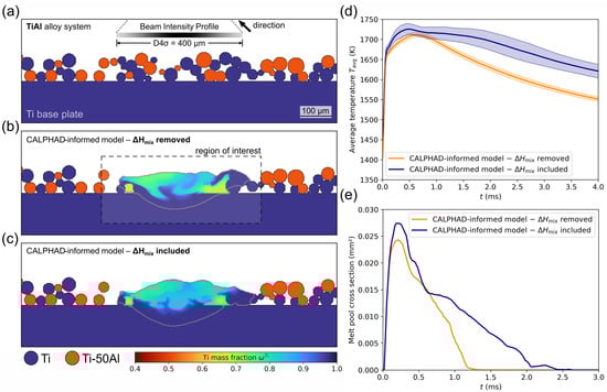
Figure 10.
Compilation of results from numerical single melt line experiments in a Ti-50Al/Ti powder mixture, simulated using the software in combination with the presented CALPHAD-informed enthalpy method. The influence of the enthalpy of mixing was analysed by removing it from the input data and comparing the results with the regular solutions, in which is considered. For a statistical analysis, the simulation was repeated five times with different powder configurations. (a) Illustration of a generated mixed powder layer, where the blue powder particles are specified as pure Ti and the orange ones exhibit a composition of Ti-50Al. (b) Resulting composition field for a case, in which is neglected. The highlighted region of interest depicts the area, in which the average temperature was evaluated. (c) Composition field for the comparative simulation, in which is considered. (d) Comparison between the averaged progressions of the mean melt track temperature for the two cases, showing that the enthalpy of mixing leads to a significant increase in temperature. (e) Temporal evolution of the melt pool cross-sections in an exemplary setup, demonstrating a substantially increased melt pool lifetime when is taken into account.
The powder layer with a height of 100 µm above the Ti base plate consisted of an equiproportional mixture between the raw materials Ti-50Al and pure Ti, as shown in Figure 10a. According to empirical values, the bulk density was set to 55%, whereas the powder size distribution was specified as Gaussian with a D50 value of about 40 µm. As the simulation results are strongly dependent on the specific powder particle configuration, the simulations were repeated five times with different randomly generated powder layers. In order to ensure that the same powder layer is present for both cases (with and without ), seed numbers were used in its generation algorithm. As indicated in Figure 10b, a small section around the melt track was chosen for the evaluation of the temperature progression because mixing processes—and therefore the effects of the enthalpy of mixing—are confined to this region. For the evaluation of the melt pool lifetime, the melt track was considered as solidified when its cross-section went below the threshold of 10% of its maximum size in order to eliminate artefacts from fluid volumes that are not in contact with the base plate.
Figure 10d shows the comparison between the mean temperature curves for the cases with and without consideration of the enthalpy of mixing. For each of the five powder configurations, the average temperature as a function of time was evaluated inside the region of interest, depicted in Figure 10b. These five curves were then averaged again for both scenarios to create the graphs in Figure 10d, where the standard deviation is illustrated by the coloured areas. The evaluation started as soon as the electron beam arrived at the simulation plane. As a result of the subsequent energy input into the material, its temperature rapidly increased until a maximum was reached. At this point, the heat flux from the melt pool arrived at the boundaries of the region of interest. After that, the ongoing heat dissipation led to a successive cooling of the melt track. By comparing the two graphs, it is clearly visible that the negative enthalpy of mixing of the TiAl alloy system leads to an exothermic mixing process, which results in a significantly higher melt pool temperature. In addition, the simulations, in which the enthalpy of mixing is considered, exhibit a larger standard deviation of . This can be traced back to the fact that the total induced enthalpy of mixing, which influences the temperature curve , is dependent on the amount of mixing that takes place in the melt pool. This, in turn, is a result of the particular powder layer configuration.
In order to obtain a reliable value for the influence of on the average melt track temperature in the examined setup, was evaluated in both scenarios at ms for all five powder layer configurations, which is summarised in Table 3. A closer look at the results shows that there are relatively large variations in the average melt line temperatures between the individual powder layers, which can be traced back to the stochastic influence of the powder distribution, which is especially pronounced when powder mixtures are used. These variations are even greater when is taken into account, as explained earlier. For the same configurations, however, the melt pool temperatures were always significantly higher in the simulations, in which is considered. In total, it was found that was (63 ± 17) K higher due to the enthalpy of mixing.
Table 3.
Overview of the simulation results for the five different powder layer variations regarding the average melt track temperature , maximum melt pool cross-section and melt pool lifetime for the single melt line simulations of the two scenarios: removed (−) and included (✓), respectively.
This temperature difference manifested itself in different progressions of the melt pool cross-sections, which are illustrated in Figure 10e. Their overall shape can be explained analogously to the temperature curves. In the simulation, in which was taken into account, the melt pool was considerably larger most of the time because the region, in which the melting temperature is exceeded, is generally larger with a higher average temperature.
For both cases (with and without ), the maximum melt pool cross-sections for the five different powder layers are displayed in Table 3. Averaged over all five tests, a maximum cross-section of (0.0250 ± 8.91 ) mm2 could be determined in the case of the neglected enthalpy of mixing. In comparison, the other scenario yielded a value of (0.0273 ± 12.6 ) mm2. This corresponds to a -induced relative increase in the maximum melt pool cross section of approximately 9%.
Far more decisive, however, is the influence of the enthalpy of mixing on the melt pool lifetime . The solidification process is much slower due to the higher maximum average melt track temperature and continuous release of heat during the liquid phase mixing, which results in a significantly higher . The data in Table 3 yield an average lifetime of (1.44 ± 0.40) ms for the case of a removed , whereas a value of (2.50 ± 0.52) ms was determined for the regular enthalpy model.
As the values vary greatly between the individual simulations, a larger study with more powder layer variations would be necessary in order to quantify the influence of the enthalpy of mixing with statistical certainty for this setup. However, the aim of this analysis was not to determine an exact value for the -based increase in , but to show that the enthalpy of mixing can have a significant influence on the melt pool lifetime. For this purpose, it is sufficient to recognise that, for each individual powder layer, the exothermic effect of leads to a strong increase in .
This insight is crucial regarding the process control during beam-based powder bed fusion processes. Three-dimensional components are usually produced using line hatching strategies, for which the melt pool lifetime is a decisive factor. This follows from the fact that different processing regimes are obtained based on and the return time of the beam [61], which is the time span necessary for the beam to return to the observed plane. With a sufficiently high melt pool lifetime, a transition of the processing regime from a trailing melt pool to a persistent melt pool occurs. The latter is characterised by the melt pool not being fully solidified when the beam of a neighbouring melt line returns to the plane, so that both melt pools join into a significantly wider liquid phase domain, which moves along the build surface perpendicularly to the melt lines. This results in highly different solidification conditions compared to the trailing melt pool regime, which can drastically influence the microstructure and properties of the produced component [62]. Thus, the results show that the enthalpy of mixing can noticeably influence the transition between these regimes, which is why this physical quantity should be taken into account in metallic multi-material simulations.
Regarding the Figure 10b,c, a qualitative comparison yields that the enthalpy of mixing has a visible influence on the composition field. However, further investigation is required to determine the underlying mechanisms in the melt pool dynamics and solidification behaviour. Although the melt pool lifetime is much higher in the simulation of Figure 10c, the mixing states seem to be relatively similar. This can most probably be traced back to the fact that the fluid velocities in the melt pool are only substantial at the beginning of the melt pool lifetime. During the subsequent solidification, the advective fluxes rapidly decrease, so that hardly any liquid phase mixing takes place after the first millisecond—in both cases. Furthermore, the melt pool envelopes, illustrated by grey lines, reveal an only slightly higher melt pool depth in the setup, which includes . This is likely the result of the relatively high heat dissipation through the start plate. Along the powder layer, however, the heat flux is lower, so that, based on the additional heat by the enthalpy of mixing, more powder particles can be molten, which is visible on the right side of the melt track in Figure 10c.
In total, this simulation example showed that the enthalpy of mixing can be an important influencing factor regarding melt pool temperatures and lifetimes. Therefore, it has to be considered to accurately predict process windows for the mentioned regimes in case of multi-material powder blends. These process-related issues will be examined in a follow-up publication.
6. Summary
The CALPHAD-based material modelling approach is already well-established in the phase-field simulation community. In this work, we show the advantages of a CALPHAD coupling for more general simulation techniques that rely on the enthalpy method to solve the evolution of the thermal field and illustrate a possible way to achieve this. The presented method is especially useful for multicomponent systems which undergo phase transitions, which often applies to physics-based simulation tools for engineering processes like metal additive manufacturing.
Our model is based on the idea of directly specifying the specific enthalpy of the considered alloy system as an input to the enthalpy balance equation instead of calculating it with a simplistic specific heat capacity approach. As an addition, the respective fluid fraction data can be used to model the solid–liquid phase transition. For the generation of the necessary datasets, it is convenient to resort to CALPHAD calculations due to the reliability of the underlying databases. In doing so, the composition and temperature-dependent enthalpy and fluid fraction is calculated prior to the actual simulation and saved in the form of plain text files. These are read into the simulation software and serve as the foundation of the material model.
As frequent conversions between enthalpy and temperature are often required, we further present robust and efficient algorithms for this task. When needed, the specific heat capacity can be directly calculated from the enthalpy data. Polymorphic and solid–liquid phase transitions pose challenges in this regard as jumps in the enthalpy data lead to immense peaks in the corresponding heat capacity. Therefore, we also elucidate ways to address different kinds of phase transitions in the context of our presented model.
The major advantage of the presented CALPHAD-informed enthalpy method is the realistic modelling of the thermophysical behaviour of metallic multicomponent systems with an implicit consideration of the enthalpy of mixing, latent heat, and highly non-linear specific heat capacity. In addition, the often complex progressions of the solidus and liquidus temperatures emerge from the fluid fraction data without the need to approximate and supply the phase diagram of the considered alloy to the simulation. Moreover, the number of necessary input parameters is greatly reduced, which makes this method less error-prone compared to conventional approaches. At the same time, the data are more reliable as the model is based on the CALPHAD method, which also comes in handy when little-studied alloy systems are considered, for which necessary material parameters are inaccessible or hard to find in the current scientific literature.
The model was applied to a lattice Boltzmann-based simulation software as well as a finite difference thermal solver. Using a diffusion couple setup, a simulation scenario for combined heat transfer and diffusion and the Stefan problem, the functionality regarding transport phenomena and solid–liquid phase transitions could be verified. Furthermore, the implicit consideration of the enthalpy of mixing and the physically required conservation of enthalpy was shown. Finally, the presented model was applied to the electron beam powder bed fusion process. By means of a Ti-50Al/Ti powder blend and single melt lines, it was shown that the enthalpy of mixing can have a significant influence on the temperature progression, cross-section and lifetime of the melt pool, which is why this effect has to be considered in simulations that cover alloying processes. For this, the presented CALPHAD-informed model is particularly well suited.
Author Contributions
Conceptualisation, R.S. and C.K.; methodology, R.S. and P.L.; software, R.S. and P.L.; validation, R.S. and P.L.; formal analysis, R.S. and M.M.; investigation, R.S. and P.L.; resources, C.K.; data curation, R.S.; writing—original draft preparation, R.S.; writing—review and editing, R.S., P.L., M.M. and C.K.; visualisation, R.S.; supervision, M.M. and C.K.; project administration, R.S.; funding acquisition, C.K. All authors have read and agreed to the published version of the manuscript.
Funding
This research was funded by the German Research Foundation (DFG) grant number KO 1984/14-1.
Data Availability Statement
The data presented in this study as well as the developed source code are available upon request from the corresponding author. The data are not publicly available due to being part of an ongoing research project.
Conflicts of Interest
The authors declare no conflicts of interest. The funders had no role in the design of the study; in the collection, analyses, or interpretation of data; in the writing of the manuscript; or in the decision to publish the results.
Nomenclature
List of used symbols and notations for physical quantities.
| Specific heat capacity | |
| Specific heat capacity of the liquid phase | |
| Specific heat capacity of the mushy zone | |
| Specific heat capacity of the solid phase | |
| Heat capacity | |
| Heat capacity of the liquid phase | |
| Heat capacity of the solid phase | |
| D | Diffusion coefficient |
| Fluid fraction | |
| h | Specific enthalpy |
| Enthalpy of mixing | |
| Specific enthalpy of mixing | |
| Normalised total specific enthalpy | |
| H | Enthalpy |
| Volume-specific enthalpy | |
| Diffusion flux | |
| l | Length |
| Diffusion length | |
| L | Latent heat of fusion |
| Thermal source term | |
| t | Time |
| T | Temperature |
| Average temperature | |
| Temperature of the liquid phase | |
| Liquidus temperature | |
| Melting point | |
| Temperature of the solid phase | |
| Solidus temperature | |
| Velocity | |
| x | Spatial coordinate |
| Position of the phase boundary | |
| Thermal diffusivity | |
| Thermal diffusivity of the liquid phase | |
| Thermal diffusivity of the solid phase | |
| Thermal conductivity | |
| Thermal conductivity of the liquid phase | |
| Thermal conductivity of the solid phase | |
| Density | |
| Density of the liquid phase | |
| Density of the solid phase | |
| Mass fraction | |
| Mass fraction of element A | |
| Mass fraction of element B | |
| Mass fraction of Chromium | |
| Composition of the liquid phase | |
| Composition of the solid phase |
References
- Kaufman, L.; Bernstein, H.L. Computer Calculation of Phase Diagrams with Special Reference to Refractory Metals; Refractory Materials. A Series of Monographs; Academic Press Inc.: New York, NY, USA, 1970. [Google Scholar]
- Saunders, N.; Miodownik, A.P. CALPHAD (Calculation of Phase Diagrams): A Comprehensive Guide; Pergamon Materials Series; Elsevier: Pergamon, UK, 1998; Volume 1. [Google Scholar]
- Lukas, H.; Fries, S.G.; Sundman, B. Computational Thermodynamics; Cambridge University Press: Cambridge, UK, 2007. [Google Scholar] [CrossRef]
- Lukas, H.; Henig, E.; Zimmermann, B. Optimization of phase diagrams by a least squares method using simultaneously different types of data. Calphad 1977, 1, 225–236. [Google Scholar] [CrossRef]
- Spencer, P. A brief history of CALPHAD. Calphad 2008, 32, 1–8. [Google Scholar] [CrossRef]
- Gaye, H.; Lupis, C. Computer calculations of multicomponent phase diagrams. Scr. Metall. 1970, 4, 685–691. [Google Scholar] [CrossRef]
- Counsell, J.F.; Lees, E.B.; Spencer, P.J. An Original Method for the Determination of Equilibrium Diagrams in Multicomponent Systems by Means of a Digital Computer. Met. Sci. J. 1971, 5, 210–213. [Google Scholar] [CrossRef]
- Grafe, U.; Böttger, B.; Tiaden, J.; Fries, S. Coupling of multicomponent thermodynamic databases to a phase field model: Application to solidification and solid state transformations of superalloys. Scr. Mater. 2000, 42, 1179–1186. [Google Scholar] [CrossRef]
- Steinbach, I.; Böttger, B.; Eiken, J.; Warnken, N.; Fries, S.G. CALPHAD and Phase-Field Modeling: A Successful Liaison. J. Phase Equilibria Diffus. 2007, 28, 101–106. [Google Scholar] [CrossRef]
- Kitashima, T. Coupling of the phase-field and CALPHAD methods for predicting multicomponent, solid-state phase transformations. Philos. Mag. 2008, 88, 1615–1637. [Google Scholar] [CrossRef]
- Steinbach, I. Second Symposium on Phase-Field Modelling in Materials Science. Int. J. Mater. Res. 2010, 101, 455. [Google Scholar] [CrossRef]
- Kattner, U.R. The CALPHAD method and its role in material and process development. Tecnol. Metal. Mater. Min. 2016, 13, 3–15. [Google Scholar] [CrossRef]
- Xiong, W.; Grönhagen, K.A.; Ågren, J.; Selleby, M.; Odqvist, J.; Chen, Q. Investigation of Spinodal Decomposition in Fe-Cr Alloys: CALPHAD Modeling and Phase Field Simulation. Solid State Phenom. 2011, 172–174, 1060–1065. [Google Scholar] [CrossRef]
- Kobayashi, H.; Ode, M.; Kim, S.G.; Kim, W.T.; Suzuki, T. Phase-field model for solidification of ternary alloys coupled with thermodynamic database. Scr. Mater. 2003, 48, 689–694. [Google Scholar] [CrossRef]
- Shamsundar, N.; Sparrow, E.M. Analysis of Multidimensional Conduction Phase Change via the Enthalpy Model. J. Heat Transf. 1975, 97, 333–340. [Google Scholar] [CrossRef]
- Date, A.W. A novel enthalpy formulation for multidimensional solidification and melting of a pure substance. Sadhana 1994, 19, 833–850. [Google Scholar] [CrossRef]
- Qin, L.; Shen, J.; Li, Q.; Shang, Z. Effects of convection patterns on freckle formation of directionally solidified Nickel-based superalloy casting with abruptly varying cross-sections. J. Cryst. Growth 2017, 466, 45–55. [Google Scholar] [CrossRef]
- Wu, M.; Liu, L.; Ding, J. An enthalpy method based on fixed-grid for quasi-steady modeling of solidification/melting processes of pure materials. Int. J. Heat Mass Transf. 2017, 108, 1383–1392. [Google Scholar] [CrossRef]
- Sudnik, W.; Radaj, D.; Erofeew, W. Computerized simulation of laser beam welding, modelling and verification. J. Phys. D Appl. Phys. 1996, 29, 2811. [Google Scholar] [CrossRef]
- Duggan, G.; Mirihanage, W.U.; Tong, M.; Browne, D.J. A combined enthalpy/front tracking method for modelling melting and solidification in laser welding. IOP Conf. Ser. Mater. Sci. Eng. 2012, 33, 012026. [Google Scholar] [CrossRef]
- Farias, R.; Teixeira, P.; Vilarinho, L. An efficient computational approach for heat source optimization in numerical simulations of arc welding processes. J. Constr. Steel Res. 2021, 176, 106382. [Google Scholar] [CrossRef]
- Attar, E.; Körner, C. Lattice Boltzmann model for thermal free surface flows with liquid–solid phase transition. Int. J. Heat Fluid Flow 2011, 32, 156–163. [Google Scholar] [CrossRef]
- Xu, P.; Xu, S.; Gao, Y.; Liu, P. A multicomponent multiphase enthalpy-based lattice Boltzmann method for droplet solidification on cold surface with different wettability. Int. J. Heat Mass Transf. 2018, 127, 136–140. [Google Scholar] [CrossRef]
- Gu, H.; Wei, C.; Li, L.; Han, Q.; Setchi, R.; Ryan, M.; Li, Q. Multi-physics modelling of molten pool development and track formation in multi-track, multi-layer and multi-material selective laser melting. Int. J. Heat Mass Transf. 2020, 151, 119458. [Google Scholar] [CrossRef]
- Zakirov, A.; Belousov, S.; Bogdanova, M.; Korneev, B.; Stepanov, A.; Perepelkina, A.; Levchenko, V.; Meshkov, A.; Potapkin, B. Predictive modeling of laser and electron beam powder bed fusion additive manufacturing of metals at the mesoscale. Addit. Manuf. 2020, 35, 101236. [Google Scholar] [CrossRef]
- Küng, V.E.; Scherr, R.; Markl, M.; Körner, C. Multi-material model for the simulation of powder bed fusion additive manufacturing. Comput. Mater. Sci. 2021, 194, 110415. [Google Scholar] [CrossRef]
- Li, E.; Wang, L.; Yu, A.; Zhou, Z. A three-phase model for simulation of heat transfer and melt pool behaviour in laser powder bed fusion process. Powder Technol. 2021, 381, 298–312. [Google Scholar] [CrossRef]
- Collins, P.; Banerjee, R.; Fraser, H. The influence of the enthalpy of mixing during the laser deposition of complex titanium alloys using elemental blends. Scr. Mater. 2003, 48, 1445–1450. [Google Scholar] [CrossRef]
- Chouhan, A.; Hesselmann, M.; Toenjes, A.; Mädler, L.; Ellendt, N. Numerical modelling of in-situ alloying of Al and Cu using the laser powder bed fusion process: A study on the effect of energy density and remelting on deposited track homogeneity. Addit. Manuf. 2022, 59, 103179. [Google Scholar] [CrossRef]
- Ohsasa, K. Numerical simulation of solidification for aluminum-base multicomponent alloy. J. Phase Equilibria 2001, 22, 498–503. [Google Scholar] [CrossRef]
- Ohsasa, K.; Shirosawa, H. Heat Transfer Analysis for Solidifying Ferrous Multi-component Alloys Using Computational Thermodynamics. ISIJ Int. 2009, 49, 1715–1721. [Google Scholar] [CrossRef][Green Version]
- Saad, A.; Gandin, C.A.; Bellet, M. Temperature-based energy solver coupled with tabulated thermodynamic properties—Application to the prediction of macrosegregation in multicomponent alloys. Comput. Mater. Sci. 2015, 99, 221–231. [Google Scholar] [CrossRef]
- Srinivas Shastri, S.; Allen, R. Method of lines and enthalpy method for solving moving boundary problems. Int. Commun. Heat Mass Transf. 1998, 25, 531–540. [Google Scholar] [CrossRef]
- Stefan, J. Über die Verdampfung und die Auflösung als Vorgänge der Diffusion. Ann. Phys. Chem. 1890, 277, 725–747. [Google Scholar] [CrossRef]
- Meyer, G.H. The numerical solution of Stefan problems with front-tracking and smoothing methods. Appl. Math. Comput. 1978, 4, 283–306. [Google Scholar] [CrossRef]
- Douglas, J., Jr.; Gallie, T.M., Jr. On the numerical integration of a parabolic differential equation subject to a moving boundary condition. Duke Math. J. 1955, 22, 557–571. [Google Scholar] [CrossRef]
- Murray, W.D.; Landis, F. Numerical and Machine Solutions of Transient Heat-Conduction Problems Involving Melting or Freezing: Part I—Method of Analysis and Sample Solutions. J. Heat Transf. 1959, 81, 106–112. [Google Scholar] [CrossRef]
- Atthey, D.R. A Finite Difference Scheme for Melting Problems. IMA J. Appl. Math. 1974, 13, 353–366. [Google Scholar] [CrossRef]
- Meyer, G.H. Multidimensional Stefan Problems. SIAM J. Numer. Anal. 1973, 10, 522–538. [Google Scholar] [CrossRef]
- Hunter, L.W.; Kuttler, J.R. The Enthalpy Method for Heat Conduction Problems With Moving Boundaries. J. Heat Transf. 1989, 111, 239–242. [Google Scholar] [CrossRef]
- Tang, C.; Yao, L.; Du, H. Computational framework for the simulation of multi material laser powder bed fusion. Int. J. Heat Mass Transf. 2022, 191, 122855. [Google Scholar] [CrossRef]
- Andersson, J.O.; Helander, T.; Höglund, L.; Shi, P.; Sundman, B. Thermo-Calc & DICTRA, computational tools for materials science. Calphad 2002, 26, 273–312. [Google Scholar] [CrossRef]
- Foundation of Computational Thermodynamics. TC-Python API Reference Documentation 2024a, 1995–2024. Available online: https://download.thermocalc.com/docs/tc-python/2024a/html/ (accessed on 13 December 2023).
- Liepold, P. CALPHAD-Basiertes Materialmodell für die Simulation der Multi-Material-Verarbeitung im EB-PBF-Prozess. Master’s Thesis, Friedrich-Alexander-Universität Erlangen-Nürnberg, Erlangen, Germany, 2021. [Google Scholar]
- Peterson, W.W. Addressing for Random-Access Storage. IBM J. Res. Dev. 1957, 1, 130–146. [Google Scholar] [CrossRef]
- Markl, M.; Rausch, A.; Küng, V.; Körner, C. SAMPLE: A Software Suite to Predict Consolidation and Microstructure for Powder Bed Fusion Additive Manufacturing. Adv. Eng. Mater. 2019, 22, 1901270. [Google Scholar] [CrossRef]
- Scherr, R.; Markl, M.; Körner, C. Volume of fluid based modeling of thermocapillary flow applied to a free surface lattice Boltzmann method. J. Comput. Phys. 2023, 492, 112441. [Google Scholar] [CrossRef]
- Chen, S.; Doolen, G.D. Lattice Boltzmann Method for Fluid Flows. Annu. Rev. Fluid Mech. 1998, 30, 329–364. [Google Scholar] [CrossRef]
- Zhang, R.; Fan, H.; Chen, H. A lattice Boltzmann approach for solving scalar transport equations. Philos. Trans. R. Soc. A Math. Phys. Eng. Sci. 2011, 369, 2264–2273. [Google Scholar] [CrossRef]
- Cook, A.W. Enthalpy diffusion in multicomponent flows. Phys. Fluids 2009, 21, 055109. [Google Scholar] [CrossRef]
- Osmanlic, F.; Körner, C. Lattice Boltzmann method for Oldroyd-B fluids. Comput. Fluids 2016, 124, 190–196. [Google Scholar] [CrossRef]
- Roache, P.J. Computational Fluid Dynamics, 1st ed.; Hermosa Publishers: Socorro, NM, USA, 1972. [Google Scholar]
- Huang, X.; Wang, L.; Jia, S.; Qian, Z.; Deng, J.; Shi, Z. Numerical Simulation of Thermal Characteristics of Anodes by Pure Metal and CuCr Alloy Material in Vacuum Arc. IEEE Trans. Plasma Sci. 2015, 43, 2283–2293. [Google Scholar] [CrossRef]
- Turchanin, M.; Nikolaenko, I. Enthalpies of solution of vanadium and chromium in liquid copper by high temperature calorimetry. J. Alloys Compd. 1996, 235, 128–132. [Google Scholar] [CrossRef]
- Turchanin, M.A. Phase equilibria and thermodynamics of binary copper systems with 3d-metals. III. Copper-chromium system. Powder Metall. Met. Ceram. 2006, 45, 457–467. [Google Scholar] [CrossRef]
- Alexiades, V.; Solomon, A.D. Mathematical Modeling of Melting and Freezing Processes; Routledge: London, UK, 2018. [Google Scholar] [CrossRef]
- Guo, D.Z.; Sun, D.L.; Li, Z.Y.; Tao, W.Q. Phase Change Heat Transfer Simulation for Boiling Bubbles Arising from a Vapor Film by the VOSET Method. Numer. Heat Transf. Part A Appl. 2011, 59, 857–881. [Google Scholar] [CrossRef]
- Ho, C.Y.; Powell, R.W.; Liley, P.E. Thermal Conductivity of the Elements. J. Phys. Chem. Ref. Data 1972, 1, 279–421. [Google Scholar] [CrossRef]
- Dinsdale, A. SGTE data for pure elements. Calphad 1991, 15, 317–425. [Google Scholar] [CrossRef]
- Klassen, A.; Bauereiß, A.; Körner, C. Modelling of electron beam absorption in complex geometries. J. Phys. D Appl. Phys. 2014, 47, 065307. [Google Scholar] [CrossRef]
- Breuning, C.; Arnold, C.; Markl, M.; Körner, C. A multivariate meltpool stability criterion for fabrication of complex geometries in electron beam powder bed fusion. Addit. Manuf. 2021, 45, 102051. [Google Scholar] [CrossRef]
- Pistor, J.; Breuning, C.; Körner, C. A Single Crystal Process Window for Electron Beam Powder Bed Fusion Additive Manufacturing of a CMSX-4 Type Ni-Based Superalloy. Materials 2021, 14, 3785. [Google Scholar] [CrossRef] [PubMed]
Disclaimer/Publisher’s Note: The statements, opinions and data contained in all publications are solely those of the individual author(s) and contributor(s) and not of MDPI and/or the editor(s). MDPI and/or the editor(s) disclaim responsibility for any injury to people or property resulting from any ideas, methods, instructions or products referred to in the content. |
© 2024 by the authors. Licensee MDPI, Basel, Switzerland. This article is an open access article distributed under the terms and conditions of the Creative Commons Attribution (CC BY) license (https://creativecommons.org/licenses/by/4.0/).