Article

Development of a Multi-Objective Optimization Tool for Screening Designs of Taut Synthetic Mooring Systems to Minimize Mooring Component Cost and Footprint

1
Advanced Structures and Composites Center, University of Maine, Orono, ME 04469, USA
2
Department of Mechanical Engineering, University of Maine, Orono, ME 04469, USA
*
Author to whom correspondence should be addressed.
Modelling 2021, 2(4), 728-752; https://doi.org/10.3390/modelling2040039
Submission received: 1 October 2021 / Revised: 24 November 2021 / Accepted: 29 November 2021 / Published: 8 December 2021
(This article belongs to the Section Modelling in Engineering Structures)

Abstract

:
As the offshore wind industry develops, more lease sites in the intermediate water depth (50–85 m) are being released to developers. In these water depths floating wind turbines with chain catenary systems and fixed-bottom turbines with jacketed structures become cost prohibitive. As such, industry and researchers have shifted focus to floating turbines with taut or semi-taut synthetic rope mooring systems. In addition to reducing the cost of the mooring systems, synthetic systems can also reduce the footprint compared to a chain catenary system which frees areas around the turbine for other maritime uses such as commercial fishing. Both the mooring systems component cost and footprint are pertinent design criteria that lend themselves naturally to a multi-objective optimization routine. In this paper a new approach for efficiently screening the design space for plausible mooring systems that balance component cost and footprint using a multi-objective genetic algorithm is presented. This method uses a tiered-constraint method to avoid performing computationally expensive time domain simulations of mooring system designs that are infeasible. Performance metrics for assessing the constraints of candidate designs are performed using open-source software such as Mooring Analysis Program (MAP++), OpenFAST and MoorDyn. A case study is presented providing a Pareto-optimal design front for a taut synthetic mooring system of a 6-MW floating offshore wind turbine.

1. Introduction

The global pipeline for floating offshore wind more than tripled in 2020 and as a result new floating technologies are needed as the industry looks to lease sites in deeper waters [1]. Currently fixed bottom jacket structures or monopiles are used in shallow waters (less than 40 m) and floating offshore wind turbines (FOWTs) with chain catenary mooring systems are used as the water gets deeper (greater than 100 m). In the intermediate water depths of roughly 55–80 m there has not been a clear solution, as fixed bottom structures and floating systems with chain catenary systems both become prohibitively expensive [2]. As researchers have worked to tackle this problem one potential solution, taut synthetic mooring systems have come to the forefront.
Taut-synthetic systems provide restoring force to the platform by the elastic properties of the rope [3]. By comparison a chain catenary system provides restoring force through the geometry of the mooring system and the weight of the chain [4]. For a chain catenary system to be functional in the intermediate depths a large amount of chain needs to be used to provide the necessary restoring force for the platform. For a taut synthetic system, it is somewhat less clear what makes a good design. Larger diameter ropes are stiffer and attract more load, but a larger diameter rope can also handle larger loads. It is also unclear what level of pretension should be used to ensure that the line can handle the loads while also not becoming slack.
Researchers have begun to develop optimization techniques to determine the best mooring systems specific to the floating platform and environmental conditions. Generally optimizing the mooring system to minimize the cost is a priority but determining if a mooring configuration is feasible is challenging. Some researchers have linearized the FOWT system and used a frequency-domain analysis [5] to estimate the response of the system or used simplified models to determine the maximum vessel responses [6], but this neglects some of the important physics such as the hull hydrodynamic load nonlinearities and fluid loading on the line. Depending on the type of mooring system, for example a chain catenary system, neglecting these nonlinear loadings can greatly under-predict the tension in the mooring lines [7].
Another approach that has been attempted is to train a surrogate-model using many time domain simulations [8,9,10]. With this approach potential mooring systems throughout the design space are simulated in the time-domain. These results are then used to build a meta-model or surrogate model where the responses of other designs in the space can be estimated by interpolating between the originally analyzed designs. With this method computational resources need to be set aside at the beginning of the optimization to generate the surrogate model, but after the model is generated, the need for computational resources decreases. Although the appropriate physics are used to generate the meta-model, there is no guarantee that the designs will behave as the meta-model predicts until a physics-based simulation is performed.
Lastly, time-domain simulations can be used for evaluating the performance of the mooring system within the optimization process [11]. Although this is the most computationally expensive of the approaches, it will lead to the most accurate results. Researchers have also experimented with screening the designs which time-domain simulations are run on to avoid wasting computational time on poor designs [10,11].
In this study a new approach is presented which continues to make the time-domain approach more computationally feasible. For this approach a tiered method for evaluating constraints is used to prevent running time domain simulations on undesirable designs. In this process progressively more restrictive constraints are evaluated to determine the effectiveness of a mooring system based on criteria like the platform natural periods which are computationally trivial compared to time-domain simulations used for determining peak mooring line tensions. Only when a design has a fair chance of success is a time domain simulation run to determine the maximum and minimum tensions in the lines. This prevents wasting unnecessary computational time on designs that were destined to fail from the beginning. The tiered constraint approach is applied in this work to optimize a taut synthetic mooring system for a 6-MW FOWT.

2. Implementation of the MOGA

The optimization technique used for this study is a multi-objective genetic algorithm (MOGA) coined the NSGA II which was developed by Deb et al. [12]. The version used here is identical to that implemented by Goupee et al. [13]. Genetic algorithms use the biological concept of survival of the fittest to find optimal solutions. In the case of multi-objective optimization there is not one optimal design, but instead a front of Pareto-optimal designs where one objective value cannot be made better without worsening another. The role of the NSGA II algorithm is to find many solutions on this Pareto front.
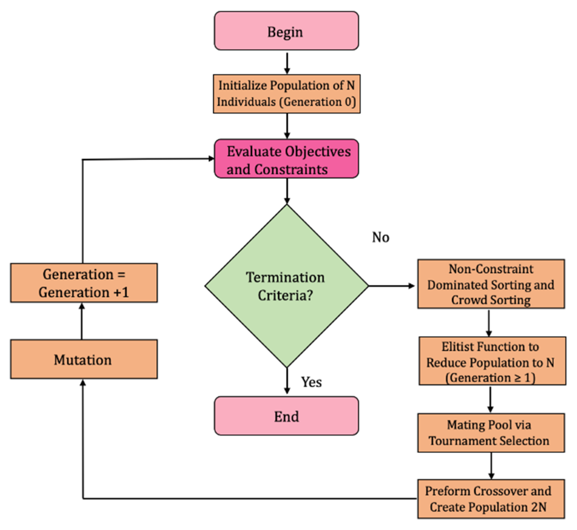
The algorithm starts by initializing a random population of individuals which represent potential solutions. These individuals have several genes which represent the various design variables. The random population is then evaluated to determine values for the multiple objectives, and if there are any constraint violations. First designs are evaluated based on the constraint violation. A member of the population with a smaller constraint value is said to be constraint dominated which encourages the optimizer to select parents that have small or zero constraint values. Next, the optimizer will prioritize designs that are non-dominated meaning the other solutions only have one objective value that is better than it while being worse in the other values. Finally, the NSGA II algorithm aims to encourage formation of the Pareto front by first favoring the non-dominated individuals and secondly favoring individuals which have a larger distance between the solutions.
After the individuals have been ranked and sorted, they are placed into a mating pool. Members of the population that have zero constraint values, are non-dominated and possess larger crowding distances are more likely to make it into the mating pool. From this pool individuals will be selected, and reproduction will occur to create new solutions called children. Reproduction consists of crossover between the individual genes, or design variables, along with occasional gene mutations. The children created then have their objective values determined, and the constraints are evaluated. This process is repeated for a set number of generations specified by the user until a Pareto-optimal front is reached. An overview of the NSGA II is shown in Figure 1.
In general, an optimization problem is expressed as finding a solution which will minimize various objective functions, while simultaneously passing constraints. Mathematically this is represented in Equation (1):
Find   x i ,   i = 1 , 2 , , V
Minimize   [ f n ( x ) ] ; n = 1 , 2 , , N
Subject   to   g p ( x ) 0 ; p = 1 , 2 , , P
where:
x is the vector of design variables;
V is the number of design variables;
f n ( x ) are the objective functions to be minimized;
N is the number of objective functions;
g p ( x ) are the constraint violations;
P is the number of inequality constraints the optimization problem is subject to.
For this problem the solution vector of design variables will include important characteristics of a mooring system for a FOWT from which other properties will be derived. The vector of design variables of interest for this problem is provided in Equation (2):
x = [ R , L s y n , d s y n , d c h a i n ]
where:
R is the mooring system radius as measured from the platform centerline;
L s y n is the length of the synthetic line (expressed as a fraction of R );
d s y n is the diameter of the synthetic line;
d c h a i n is the chain diameter.
This optimization problem will feature two objective functions that are of importance for a FOWT mooring system, cost and mooring radius. Reducing cost for any renewable energy application is of utmost importance to ensure that the technology is economically feasible. In addition, it is crucial to try and minimize the radius, and by extension footprint, of the FOWT to minimize environmental impacts and impacts on other ocean uses such as fishing. For a multi-objective optimization routine to work successfully it is important to ensure that the two objectives are competing. At first glance it would seem as though these objectives are not competing as smaller mooring radii have smaller corresponding line lengths which will be less expensive. However, there are two trends that cause larger mooring radii to ultimately be cheaper for taut systems based on initial designs that were generated [14]. First, for a taut mooring system as the mooring radius increases the line length will also increase effectively reducing the stiffness of the mooring system for the same line stiffness (EA). This softer system will lead to the mooring system attracting less loads which will ultimately require a smaller diameter line. Second, as the mooring system radius increases the line becomes more horizontal which makes it better able to resist platform motions. Mathematically, the multi-objective minimization problem is stated in Equation (3):
Minimize   [ f 1 ( x ) , f 2 ( x ) ]
Subject   to :   g i ( x ) 0 ,   i = 1 , 2 , , 6
210   m R 290   m
0.68 L s y n 0.80
100   mm d s y n 192   mm
100   mm d c h a i n 177   mm
where:
f 1 ( x ) is the mooring system radius;
f 2 ( x ) is the mooring system component cost;
g 1 ( x ) is the mooring system geometric constraint violation;
g 2 ( x ) is the platform heave natural period constraint;
g 3 ( x ) is the platform pitch natural period constraint;
g 4 ( x ) is the maximum chain tension constraint;
g 5 ( x ) is the maximum synthetic tension constraint;
g 6 ( x ) is the minimum synthetic tension constraint.
The constraints for this optimization problem ensure that the mooring system being analyzed is a valid solution. Many of these constraints are based on the ABS/IEC guidelines for designing and simulating floating offshore wind turbines, but time-domain simulations are very computationally expensive. To avoid running time-domain simulations, if possible, a tiered constraint system has been implemented where simpler and more computationally efficient constraints are used to screen potential designs. If the simple constraints are not met this indicates that the design would not be worth analyzing in the time domain. At a high level the constraints and their order from simple to complex are as follows:
(1)
A geometric feasibility constraint is implemented to avoid analyzing designs where the line lengths for a certain mooring radius yield nonsensical designs (i.e., g 1 ( x ) ).
(2)
Next, the FOWT platform periods are estimated so that designs which do meet minimum natural period requirements and would likely have resonance issues due to the wave loading are not analyzed (i.e., g 2 ( x )   and   g 3 ( x ) ).
(3)
Designs which pass the aforementioned constraints are subjected to DLC 6.1 simulations to determine the maximum and minimum loads in the mooring system and assess constraints requiring these values (i.e., g 4 ( x ) g 6 ( x ) ).
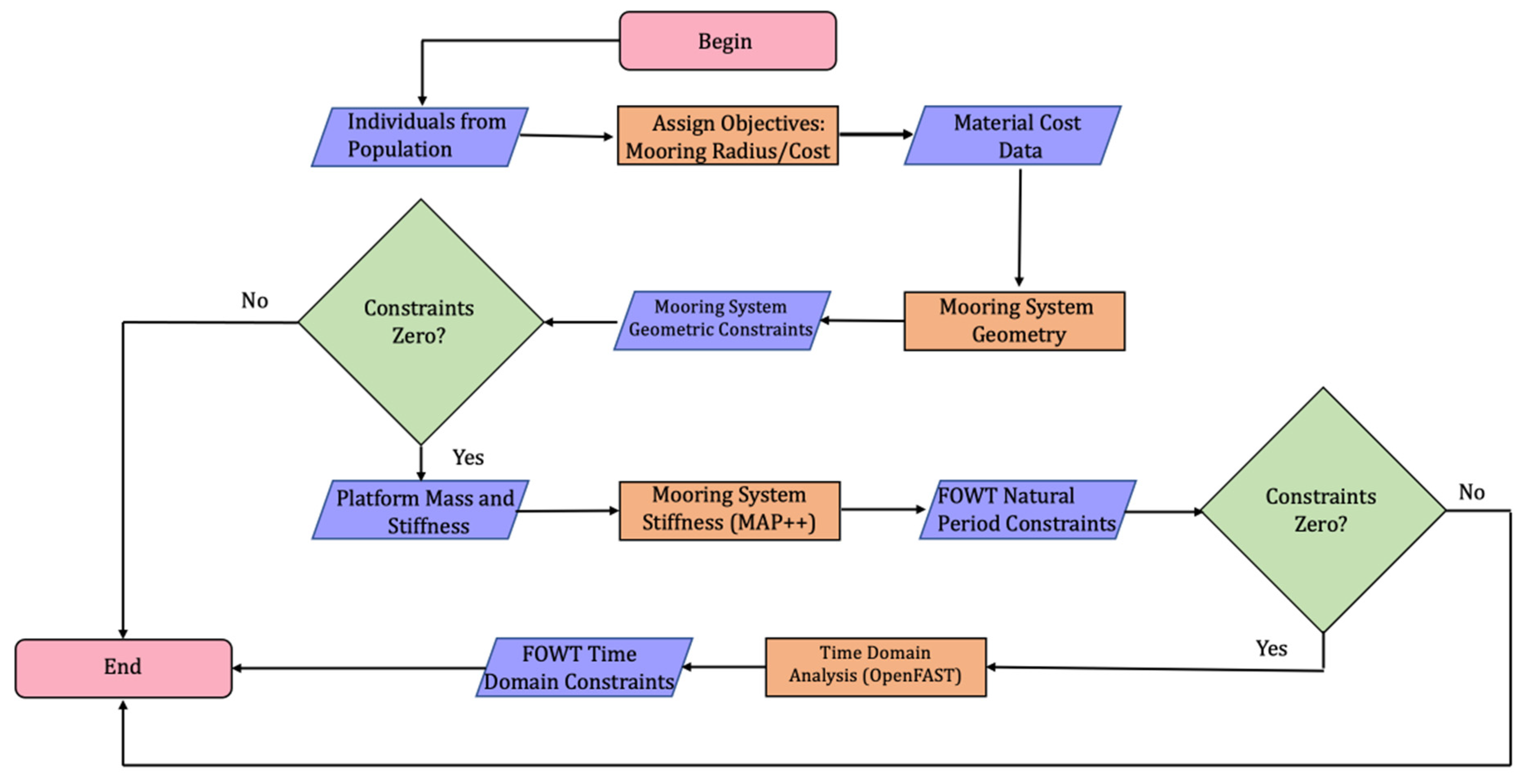
The various constraints are posed in such a way that failing earlier on in the screening process leads to larger constraint violations, thus encouraging the optimizer to favor designs that make it further into the screening process. A flow chart illustrating how the objective functions and constraints are calculated is provided in Figure 2. The mathematical specifics of the constraints are discussed in the subsequent text.
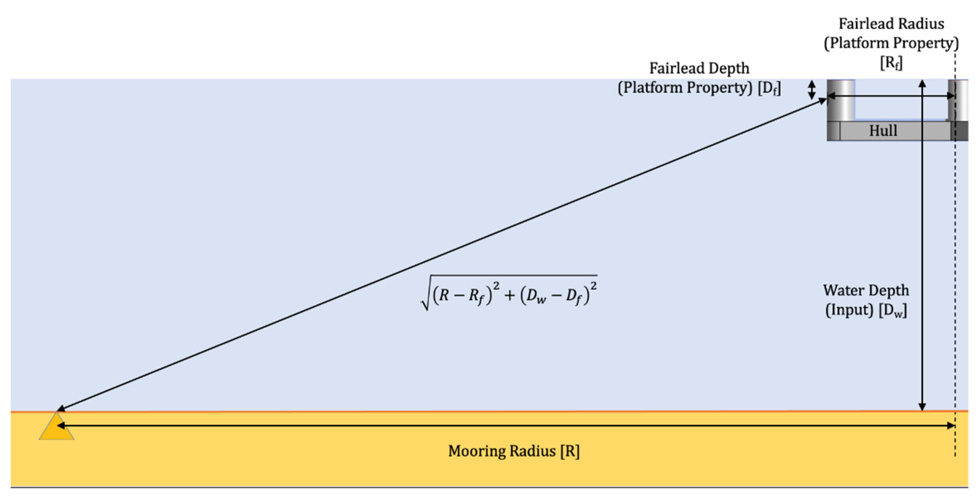
The first constraint considered in Figure 2 is whether the mooring system is geometrically feasible. There are two obvious scenarios where the mooring system would be geometrically infeasible and lead to constraint violations. The first is the situation where there is no horizontal component to the reaction in the line. A line that goes directly from the fairlead connection point vertically to the seafloor will not provide a restoring force so any line length that is greater than the sum of the distance from the fairlead depth to the seafloor and the fairlead radius to the anchor radius will be considered an invalid solution and penalized accordingly. Similarly, there is a maximum level of prestrain in a synthetic line for which the dynamics of the turbine will not be handled. Generally, it would not be feasible to have a line which has a prestrain more than roughly 10%. As such, line length less than approximately 90% of the straight-line distance between the fairlead and anchor connections are also subject to a large constraint violation. Depending on the synthetic materials used for analysis this percentage could change. For example, an extremely stiff synthetic material such as Dyneema would only be feasible for a much lower prestrain. The mooring system schematic illustrating the mooring system and platform geometry needed to determine if a design meets this geometric feasibility constraint is illustrated in Figure 3.
For the constraints to guide the optimizer towards feasible solutions they must be carefully constructed. The minimum line length geometric constraint is provided in Equations (4) and (5). The constraint violation is crafted in such a way that a line that is just barely infeasible, such as a line prestrain of 11%, will have a smaller constraint violation than more egregious designs which will yield larger constraint violations. In this way the design variable vector will be guided towards feasible solutions. The maximum line length geometric constraint is constructed in a very similar way to ensure that the optimizer is guided towards good designs. If the mooring system fails these initial constraints, it will not be worth evaluating the more computationally expensive constraints, and these poor designs will be screened out immediately.
If :   L T 0.9 ( R R f ) 2 + ( D w D f ) 2
Then :   g 1 = 100 0.9 ( R R f ) 2 + ( D w D f ) 2 L T 0.9 ( R R f ) 2 + ( D w D f ) 2 + 100
Else :   g 1 = 0
If :   ( R R f ) + ( D w D f ) L T
Then :   g 1 = 100 L T [ ( R R f ) + ( D w D f ) ] [ ( R R f ) + ( D w D f ) ] + 100
Else :   g 1 = 0
where:
R f is the distance from the center of the platform to the fairlead connection point;
D w is water depth;
D f is the depth from the mean water line (MWL) to the fairlead connection point;
L T is the total line length.
The next constraints to check are the rigid-body natural periods of the platform. If the heave and pitch natural periods of the platform are too close to typical periods of ocean waves it is more likely that the platform motion will experience resonance increasing loads throughout the FOWT, and thus, the mooring system design would be unsatisfactory. To calculate the natural periods for heave and pitch as shown in Equations (6) and (7), the stiffnesses due to the hydrostatic restoring force and mooring system stiffness as well as the mass/inertia and added mass/inertia properties of the platform are needed. All the quantities except the mooring system stiffness are from the turbine and tower masses and locations as well as the platform mass and dimensions. The mooring system stiffness is determined using Mooring Analysis Program (MAP++).
MAP++ [15] is a quasi-static catenary line solver which is more computationally efficient then a lumped mass model such as MoorDyn [16] which will be used for the time domain simulations. It can be used within OpenFAST [
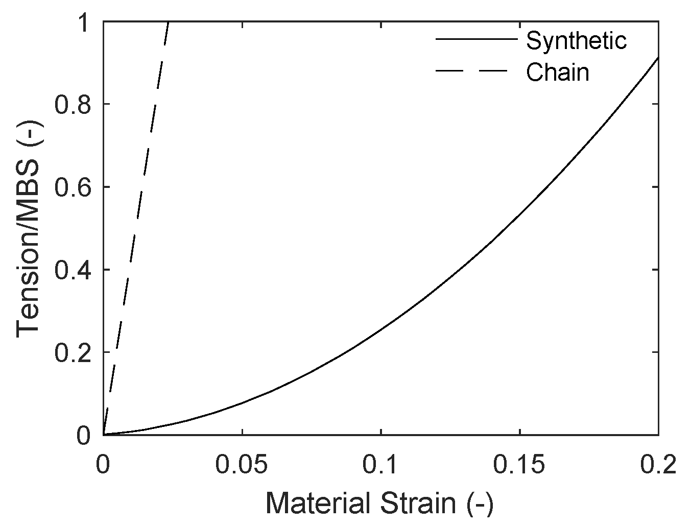
17] to model a mooring system or can be called on its own to determine properties like the 6 × 6 mooring system stiffness matrix. The one downside to MAP++ is that it only allows linear elastic materials in the mooring system. As a result, it is important to estimate the stiffness of the synthetic segment of the mooring line at the corresponding installed strain. This approach will lead to a mooring system that has the right stiffness characteristics about the undisplaced position of the FOWT which is sufficient for computing natural frequencies.
As with the geometric constraints the constraint values have been carefully crafted to return smaller values for natural periods that are closer to the specified values in order to drive the vector of design variables towards a feasible solution. The total constraint violation for the natural periods will be the sum of the constraint violations calculated in Equations (6) and (7).
T n _ heave = 2 π k 33 + k 33 Mooring m platform + a 33
If :   T n _ heave 18
Then :   g 2 = 30 18 T n _ heave 18 + 50
Else :   g 2 = 0
where:
k 33 is the platform heave stiffness;
k 33 Mooring is the mooring system heave stiffness;
m platform is the mass of the platform;
a 33 is the infinite period added mass of the platform in heave;
T n _ heave is the platform heave natural period.
T n _ pitch = 2 π k 55 + k 55 Mooring I platform + a 55
If :   T n _ pitch 25
Then :   g 3 = 30 25 T n _ pitch 25 + 50
Else :   g 3 = 0
where:
k 55 is the platform pitch stiffness;
k 55 Mooring is the mooring system pitch stiffness;
I platform is the platform pitch inertia;
a 55 is the infinite period added inertia of the platform in pitch;
T n _ pitch is the platform pitch natural period.
If the previous constraints are not violated by the mooring system a time-domain simulation is run in OpenFAST to check the tensions in the lines due to ultimate loading. This includes checking the tension both at the chain fairlead and in the synthetic section to ensure that the line tension is below the line MBS with the appropriate ABS/IEC factors of safety, as well as ensuring that the tension in the synthetic section does not go slack. The constraint violations for the tension in the chain leader are given by Equation (8) and the constraint violation for the maximum tension in the synthetic segment is given by Equation (9). The last of the constraints to be checked is the minimum synthetic tension requirement given in Equation (10).
If :   F f _ chain   T fairlead _ max MBS chain
Then : g 4 = F f _ chain   T fairlead _ max MBS chain MBS chain
Else : g 4 = 0
where:
T fairlead _ max is the maximum tension at the fairlead;
F f _ chain is chain fatigue factor;
MBS chain is the minimum breaking strength of the chain.
If :   F s _ syn T syn _ max MBS syn
Then : g 5 =   F s _ syn T syn _ max MBS syn MBS syn
Else : g 5 = 0
where:
T syn _ max is the maximum tension at the fairlead;
F s _ syn is the ABS synthetic factor of safety for a synthetic;
MBS syn is the minimum breaking strength of the synthetic.
If :   T syn _ min F min _ syn · MBS syn
Then : g 6 = F min _ syn   MBS syn T syn _ min F min _ syn · MBS syn
Else : g 6 = 0
where:
T syn _ min is the minimum tension at the fairlead;
F min _ syn is the minimum allowable line tension to avoid slack lines as a percentage of MBS.
The last part of the constraint violations that is worth discussing is the constant added to the geometric and natural period constraint violations. These are crafted to guide the optimizer toward more suitable solutions. In this case a design which fails the geometric constraint will automatically be larger than any designs that fail the natural period constraint or the time-domain constraints. As designs that fail the geometric constraints will be especially poor designs this will guide the optimizer towards solutions that are at least evaluated for the natural periods and/or in the time domain. Similarly, a design which fails one of the natural period constraints will always be larger than a design which makes it through to the time domain simulations. This ensured that the optimizer always favors designs that made it further in the process which helps the optimizer find feasible solutions while also avoiding computationally taxing time domain simulations of poor designs.

3. Optimization Inputs

To perform an optimization for a FOWT mooring system a few key inputs are necessary. First, mooring line property and cost data for both the chain and the synthetic materials are provided. In the case of synthetics, the nonlinear tension-strain response of the line are key inputs and crucial to obtaining the correct mooring line responses. The second key input is the FOWT properties including the location of the center of gravity and mass of various components such as the tower, turbine, and platform. In addition, the hydrodynamic properties of the floater are needed. Lastly, the design criteria such as factors of safety, and the environmental loading on the turbine including the wind, wave and current loading necessary for performing the optimization are provided.
For this case study a taut synthetic mooring system for a 6-MW turbine based on the University of Maine’s VolturnUS floating platform will be optimized to minimize the mooring footprint and component cost. This turbine will be subject to the ABS/IEC DLC 6.1 conditions associated with the University of Maine Monhegan test site.

3.1. Mooring System

The mooring system to be optimized is a taut synthetic system. This system includes a chain leader at the fairlead as well as chain at the anchor as required by ABS to mitigate Ultra-Violet (UV) and sediment damage respectively. A design schematic for the mooring configuration described is provided in Figure 4.
For this optimization case study, the chain leaders at the top and bottom of the mooring line were fixed at 10 m each and both were required to have the same chain diameter which could range from 100 mm to 177 mm. The synthetic diameter could range from 100 mm to 192 mm as long as the design constraints were met. The mooring system properties for this configuration including the fairlead connection points on the platform and orientation of the mooring lines are provided in Table 1.
Synthetic lines exhibit a nonlinear tension-strain response that is important to account for when designing a system. A modified version of OpenFAST that has been validated against experimental data is used to incorporate the nonlinear behavior [18]. In this modified version of OpenFAST a general line tension strain response can be input into the model via a lookup table. For this problem the synthetic and chain tension-strain curves are provided in Figure 5. Note that both the synthetic and chain tension-strain responses provided are non-dimensionalized based on the line MBS.
The chain and synthetic load capacity and mass properties are provided in Figure 6. The mass properties provided are the line dry mass per unit length. The specific gravity of the synthetic mooring lines is 1.15.
The last piece of data needed to optimize the mooring system is the cost data for each of the line components which is provided in Table 2. For this optimization only the mooring line component cost will be minimized so connections, installation and anchor costs will not be included. In future work the optimizer will be expanded to account for these other costs, but where the designs are similar it will be assumed that these costs not accounted for will be similar across the various designs.

3.2. Description of the Turbine

For this study a 6-MW turbine based on the University of Maine VolturnUS technology is used. The VolturnUS platform is a concrete semi-submersible design with three radial columns providing stability and a center column which the turbine is mounted to. Three pontoons connecting the columns also serve as ballast tanks which can be filled with seawater to ensure that the draft of the platform is 20 m. The dimensions of the VolturnUS 6-MW floating platform are provided in Figure 7.
OpenFAST uses hydrodynamic information from a potential flow solver, WAMIT [19], to solve for the forcing on the hull as well as the frequency-dependent added mass and damping coefficients. WAMIT solves the frequency-domain potential flow wave-structure interaction problem using a panel-based method with the appropriate boundary conditions. The hydrostatic stiffness matrix as well as the infinite-period added mass matrix are needed to estimate the natural periods of the structure and are obtained from the potential flow analysis using the submerged geometry of the 6-MW VolturnUS platform. WAMIT provides the stiffness contribution due to both the waterplane area and the center of buoyancy, but the center of gravity contribution is handled separately in OpenFAST by finding the component masses and locations, some of which are deformable, and using those to compute the FOWT weight and center of gravity at any instant in time. The FOWT mass properties are provided in Table 3.

3.3. Design Criteria

The design criteria for FOWT installations are provided by the American Bureau of Shipping (ABS) classing agency and International Electrotechnical Commission (IEC) standards organization. Certain extreme design load cases (DLCs), such as DLC 6.1 the 50-year extreme storm environment, are commonly found to dictate the size of the mooring system [20,21]. For this DLC, ABS/IEC require that six simulations of at least one-hour duration be analyzed with different random conditions representing the turbulent wind field and irregular wave field, and the mooring line design value is based on mean of the maximum mooring line response from these six simulations.
In addition to the DLCs of importance, the classing agencies also give guidance on the material factors of safety to be used and other requirements of the mooring system. For a taut synthetic mooring system with non-redundant mooring lines the material factor of safety is 2.184. This value is derived from a synthetic material factor of safety of 1.82 which is increased by 20% for a non-redundant mooring system [21,22,23]. Fatigue damage for synthetic ropes is not a concern because the steel connections are far more susceptible to fatigue failure. The guidelines also require that the synthetic section be submerged to mitigate UV damage [24] and kept off the seafloor to prevent coarse sand and dirt from becoming embedded in the rope and damaging it. This requires chain leaders to be installed at both the anchor side and fairlead side of the mooring system.
In addition to the maximum tension requirements, the classing agencies also prohibit slack line events for certain synthetic materials. With this requirement there is some flexibility, and it is not explicitly stated what that would entail for synthetics such as nylon and polyester. Guidance, however, is given for aramid fiber ropes which have failed on oil and gas platforms due to the phenomenon of axial compressive fatigue [22,25]. To prevent that from occurring in those types of synthetic fiber ropes it is required that the minimum load in the line stay above 2% of the minimum breaking strength (MBS) of the line. Although this value is likely conservative for materials such as nylon and polyester which do not risk failure due to the axial fatigue phenomenon, it is applied here to ensure a robust design. The design requirements in this work are summarized in Table 4.
The second value from Table 1, the minimum chain factor of safety used, does not follow directly from design standards. This value was derived from a fully designed and ABS-approved [26] chain catenary mooring system for the same platform and environmental conditions. To obtain this value the 100% ABS approved catenary system was simulated according to DLCs 1.2 (operational wind turbine with associated wave conditions), which makes up most of the fatigue damage conditions for the mooring system, and DLC 6.1 which is assumed to control ultimate limit state design. The minimum breaking strength required for a given chain size to satisfy the DLC 1.2 conditions was divided by the minimum breaking strength required to satisfy the DLC 6.1 conditions, resulting in a fatigue factor. Such a factor is used to estimate chain sizes that would satisfy fatigue requirements after only running DLC 6.1.
The last values presented in the table are the minimum platform periods. If the mooring system has a surge period less than 40 s it is extremely likely that the mooring system will be overly stiff and attract large loads to the mooring system requiring larger mooring components. The minimum heave and pitch periods are dictated by the wave loading on the platform. If the mooring system adds too much stiffness to heave and pitch responses the platform responses could get too close to wave energy periods leading to resonance issues with the FOWT and excessive wind turbine loads and accelerations.

3.4. Environmental Loading

The environmental loading applied to the model is due to wind, wave, and current loading for the ABS DLC 6.1 50-year event. The wave loading applied to the structure is based on the University of Maine Monhegan test site [27]. For the VolturnUS system at this location the ABS/IEC DLC 6.1 is the driving load case for ultimate loads. Although the Survival Load Case (SLC) has a larger associated significant wave height of 12.0 m vs. 10.2 m [28] the partial safety factors for normal and abnormal loading are specified by ABS/IEC by 1.35 and 1.1, respectively. This leads to the DLC 6.1 factored loads being larger than the SLC loads [29].
The environmental loading is applied at both 0 degrees and 180 degrees to produce the largest and smallest loads in the front line parallel to the environmental loading directions, respectively. The DLC 6.1 environment including the parameters that describe the JONSWAP wave spectrum (significant wave height, peak period and a shape parameter) as well as the mean loads due to wind, second order wave and current is provided in Table 5.
Generally, DLC 6.1 requires applying a turbulent wind field to the FOWT which requires that the simulations use small timesteps (~10 ms) to resolve high frequency responses in the structure. To avoid unnecessary computational expense, tower and blade degree of freedoms in OpenFAST were disabled, and the aerodynamic loading was applied as a mean load. These responses likely will only marginally influence mooring line tensions, which ultimately dictate the design of the mooring system components. The mooring system tensions are driven largely by the motion of the platform, which has low rigid-body natural frequencies and whose motions are well predicted even with large timesteps.
Similarly, the low-frequency and second order wave response is approximated by applying a mean load onto the FOWT. It is possible to model these responses in OpenFAST using second-order sum and difference frequency quadratic-transfer functions (QTFs) but during initialization it takes OpenFAST ~40 s to read in the QTFs which will quickly make the problem computationally infeasible on the average desktop computer with four cores. Ideally, with sufficient computational resources the time domain simulations would be performed with both a turbulent wind field and the full second-order QTFs, but for computational efficiency the mean load due to the second order-wave effects was determined by using only the diagonal terms of the difference QTF and the wave heights from the JONSWAP spectrum as outlined in DNV’s Global Performance of Deepwater Floating Structures [30].

4. Accelerating the Simulation Process for Obtaining Design Constraint Values

With enough computational resources designs generated with the optimization process outlined in this paper could follow the guidance provided by the ABS/IEC including running all the required DLCs. Unfortunately, this is computationally infeasible with the computational resources used in this study and instead one of the design-driving load conditions, DLC 6.1 the 50-year wind and wave loading, is chosen as the controlling design scenario. Even running only one DLC requires many seeds and wind/wave headings and for this design that would include six one-hour simulations as required by ABS. To induce both the maximum and minimum responses in the lead line this would require two DLC 6.1 runs, 0 and 180 degrees, and would bring the total number of one-hour simulations to 12. Unfortunately, even with the simplifications made to the environmental loading by modeling the current, second-order wave loading and wind loading as a mean load the problem is still too computationally expensive with normal computational resources. To make the problem posed more computationally tractable on an average desktop computer with four cores, several approaches were applied that reduced computational time during the optimization process.

4.1. Extrapolating the Maximum DLC 6.1 Line Response Based on a Shorter Simulation Time

Ideally all six one-hour simulations would be run for the 0- and 180-degree loading scenarios, and this could be done given the right computational resources. The maximum and minimum tension response in the line is estimated based on a generalized extreme value (GEV) fit of a shortened simulation, and second a seed is carefully selected such that the maximum tension response in the line closely matches the DLC 6.1 maximum design load obtained from the full complement of full-length simulations. In order to select this seed, the maximum line tension design load is found using the ABS/IEC design guidelines for a representative design that involves taking the mean of the maximum tensions from six one-hour simulations using randomly generated seeds to generate the JONSWAP wave spectra. The DLC 6.1 simulations were run on a representative design for a taut nylon moorings system deployed in a water depth of 55 m with a mooring radius of 205 m [20]. The results of these simulations including the randomly generated seeds and line tensions statistics used in this work are presented in Table 6.
The smallest and largest maximum line tension simulated by OpenFAST for the six one-hour simulations was 2362 kN and 3318 kN, respectively. The maximum line tension used for design is the average of these six runs or 2751 kN. The coefficient of variation of the mean load in the line is 0.2% which is expected since the mean environmental load is the same for all simulations. Lastly, the coefficient of variation for the line tension standard deviation is 5.4% which signals that each simulation contains a similar amount of energy from the environmental loads. This is also to be expected as a JONSWAP spectrum with different seeds should induce a similar statistical response to the platform with sufficient simulation time.
Before the simulation results could be fit to a statistical distribution the tension peaks from the mooring line tension time history had to be extracted. To ensure the selected data points are truly peaks the data was first smoothed using a Savitzky-Golay Filter by calling MATLABs built in function sgolay. This ensures that small numerical errors from OpenFAST are not selected as peaks and that peaks are not accounted for more than one time. It is also important that the method for searching for peaks is repeatable across different mooring designs. For this problem it was found that searching for peaks where the minimum peak prominence was two times the standard deviation of the line tension signal would return good results. In this context, minimum peak prominence was found by comparing the local maximum to the local minimums on either side, and the smaller of the differences between the local maxima and minima is defined as the prominence. The peaks in the signal were determined using MATLABs built in function findpeaks.
Once the peaks of the mooring line tension response were determined a GEV distribution was fit to the peaks as illustrated in Figure 8. The empirical cumulative density function matches the GEV distribution well and stays within the 95% confidence intervals providing evidence that the GEV is a good statistical fit for this data.
The maximum tension response in the mooring line was extrapolated using 1000 s worth of data. To extrapolate the maximum tension in the mooring line all the peaks in the signal during the 1000 s simulation were counted. The number of peaks were then used to estimate the number of peaks that would occur in a one-hour simulation, and the GEV distribution was fit to the tension peaks of 1000 s worth of data. Using the estimated peaks that would occur in the signal the probability of the maximum event was determined, and this probability was used with the GEV cumulative distribution function to estimate the maximum tension response in the line. The results of using this method of 1000 s used to estimate the tension response is presented in Table 7.
The DLC 6.1 design value for tension in the mooring line was 2751 kN based on the mean of the maximum line responses for the six–one-hour simulations, and the value extrapolated from the first 1000 s of seed A, 2810 kN, is close to the design value. One thousand seconds of Seed A in tandem with extrapolating the maximum tension response in the line returned a tension that was 2% larger than the ABS derived DLC 6.1 design value. This particular seed and the proposed extrapolation approach were used to evaluate mooring system design constraints requiring peak (or minimum) tensions. Its once again worth noting that more accurate peak values could be obtained by running the full suite of full-length simulations in the optimizer and would be recommended if the computational resources were available.

4.2. Selection of OpenFAST and MoorDyn Timesteps

Another important and non-trivial simulation setting is the selection of OpenFAST and MoorDyn timesteps as well as the discretization of the mooring line. Smaller timesteps will provide more accuracy in the solution at the expense of more computational resources. It was also found through testing that the OpenFAST and MoorDyn timesteps have a dependency on each other. For a given OpenFAST timestep and a taut-synthetic mooring configuration with 10 m of chain at the anchor and fairlead there is a limit on how small the MoorDyn timestep can become, and if it is too small, the model loses numerical stability. This may be due to the soft coupling that is used within OpenFAST where the physics of the mooring line and the platform motions are solved separately of one another, and information is passed between each solver through the OpenFAST glue code. Another plausible explanation for this observation could be due to high-frequency axial models of vibration in the line that can only be resolved with a sufficiently small timestep.
To determine the right level of mooring line discretization in tandem with the appropriate OpenFAST and MoorDyn timesteps a convergence study was undertaken. In this convergence study the line was discretized into 10, 40 and 160 lumped masses and the MoorDyn and OpenFAST timesteps were determined based on the highest estimated natural frequency of the line. The OpenFAST and MoorDyn timesteps used in this study are provided in Table 8.
With the discretization scheme provided a grid can be constructed in which quantities of interest such as line tension and platform displacements can be determined. For these convergence studies 1000 s of simulation with 250 s of dumped transients was used to determine the FOWT’s maximum response. One way to visualize these results is through a surface plot like the one for the line maximum tension presented in Figure 9.
As can be seen from the three surfaces plotted in Figure 9 mooring systems with a coarser discretization can be simulated with more aggressive OpenFAST and MoorDyn timesteps with reasonable accuracy saving on computational efficiency. For the taut synthetic systems being modeled, the internal line tension will be much larger than the inertial force of the line as well as the fluid loading on the line. This is due to the line having a small mass resulting from the use of synthetic materials and having relatively small motions relative to the fluid. If the system being optimized was a chain catenary system the mooring lines would likely need to be discretized more finely to capture the line inertia and the fluid loading, which are very substantial for that type of system. Table 9 compares the selected mooring discretization with 10 lumped masses and the selected OpenFAST and MoorDyn timesteps of 0.175 s and 2.5 ms respectively to the converged values for platform and mooring system properties of interest.
With the selected MoorDyn and OpenFAST settings it is possible to run the simulation quickly and still maintain a good amount of accuracy as all quantities investigated are within 5% of the converged values. The values that are most important to the design, the mooring line tensions, vary from 2.7% too large to 2.8% too low relative to the high node count, small timestep simulation which is very reasonable considering the coarse line discretization and the large OpenFAST timestep used.

5. MOGA Mooring Optimization Results

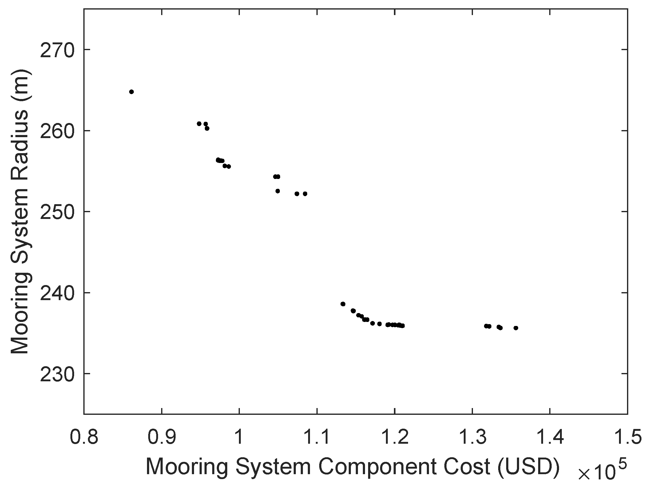
Using the optimization procedure outlined a mooring system was optimized for the VolturnUS 6-MW system provided. The aim of the optimization was to find feasible designs that passed the ABS 6.1 50-year wind and wave loading by using the constraint screening method and computational improvements outlined in this paper. The optimum designs in terms of mooring radius and mooring line component cost generated by the MOGA are shown in Figure 10. These designs were generated with a population of 180 individuals that were run for a total of 200 generations, and even with the performance enhancements implemented, the algorithm took ~7 days to run. The Pareto front shows that to have a FOWT with a smaller mooring radius a larger capital investment must be made in the mooring system. The cheapest design along this front has a component cost of approximately 86,000 USD and has a radius of about 265 m. As the radius of the mooring system is decreased the cost increases in a somewhat linear fashion to a design which has a cost of 108,000 USD and corresponding radius of about 252 m. At this point there is a jump in the Pareto front until a design which has a radius of 239 m and a cost of 113,000 dollars. After this jump in the Pareto front, mooring system radius can be reduced in radius slightly to about 235 m, but this 4 m reduction comes at a large increase in price.
The optimization performed started with 180 randomly generated individuals of which there were no restrictions on the initial seeding in the population. The constraint values were determined through the tiered-constraint method presented which was designed to both avoid running time domain simulations on infeasible designs, and to guide the optimizer towards feasible designs. This optimization was run several times with similar results observed including the jump in the Pareto front.
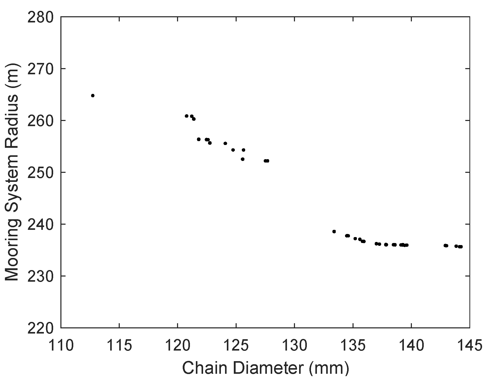
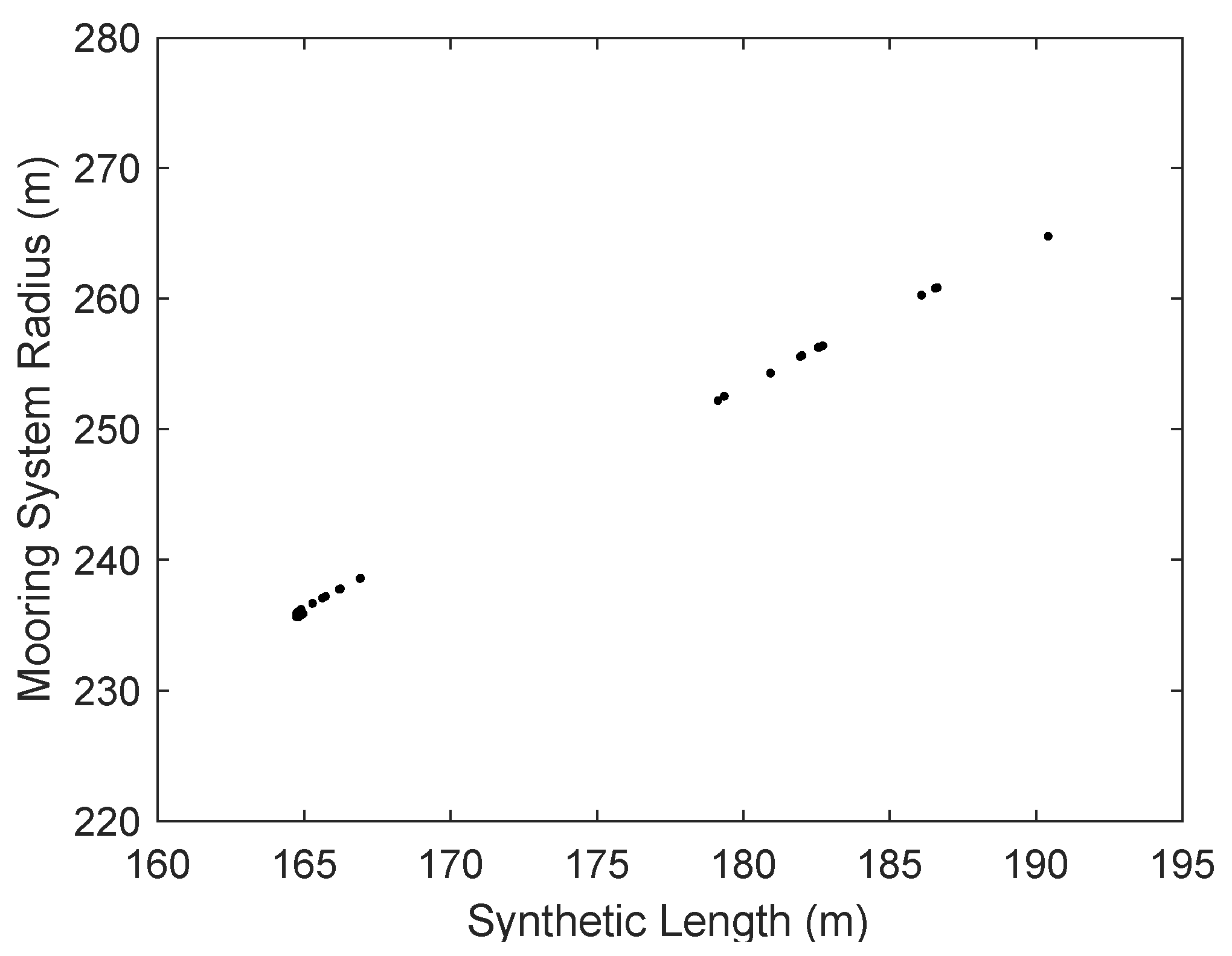
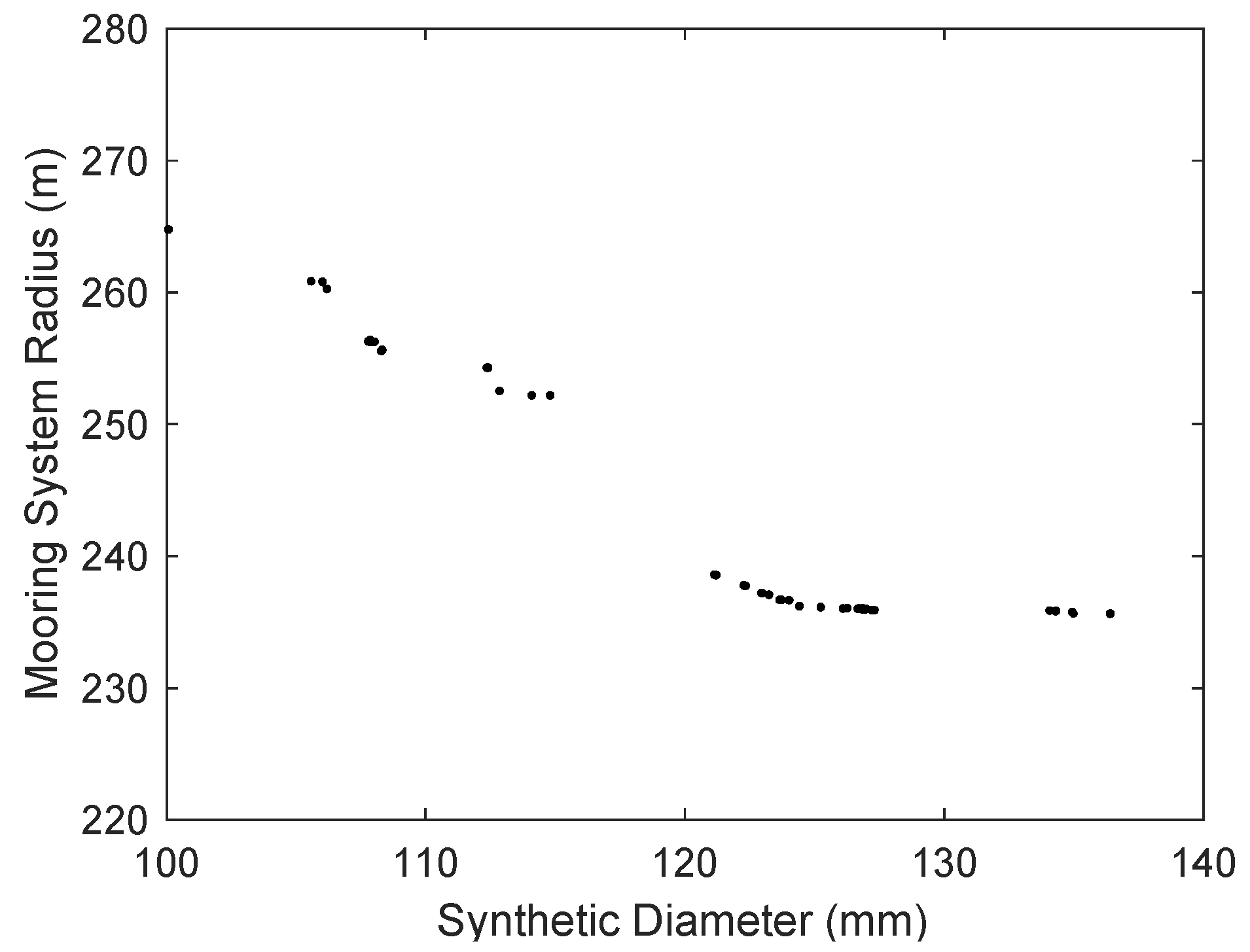
In this optimization problem one of the objectives, mooring system component cost, is a function of chain diameter, synthetic length and synthetic diameter. To gain a better understanding of the relationship between mooring system radius with respect to these variables plots are provided for mooring system radius vs. synthetic line length, chain diameter and synthetic diameter in Figure 11, Figure 12 and Figure 13, respectively.
Figure 11 shows that the synthetic segment length increases with the mooring radius in a nearly linear fashion. This makes sense as one of the constraints of the mooring system is to keep the line tensions below a certain maximum, but it is also important to keep the tensions above a certain threshold to prevent slack lines. To maintain this balance the optimizer will need to increase the synthetic line length as the mooring radius increases
The second phenomenon illustrated in both Figure 12 and Figure 13 is the decrease in line diameter as mooring radius increases. This is likely due to two different effects acting in concert. First as mooring system radius increases so does mooring line length. As a result, the effective stiffness of each mooring line as well as the whole mooring system stiffness will decrease which will attract less loads necessitating smaller lines. In addition, as the radius increases the mooring line becomes more horizontal leading to a larger portion of the line tension vector counteracting the applied mean environmental load, in turn, resulting in smaller lines.
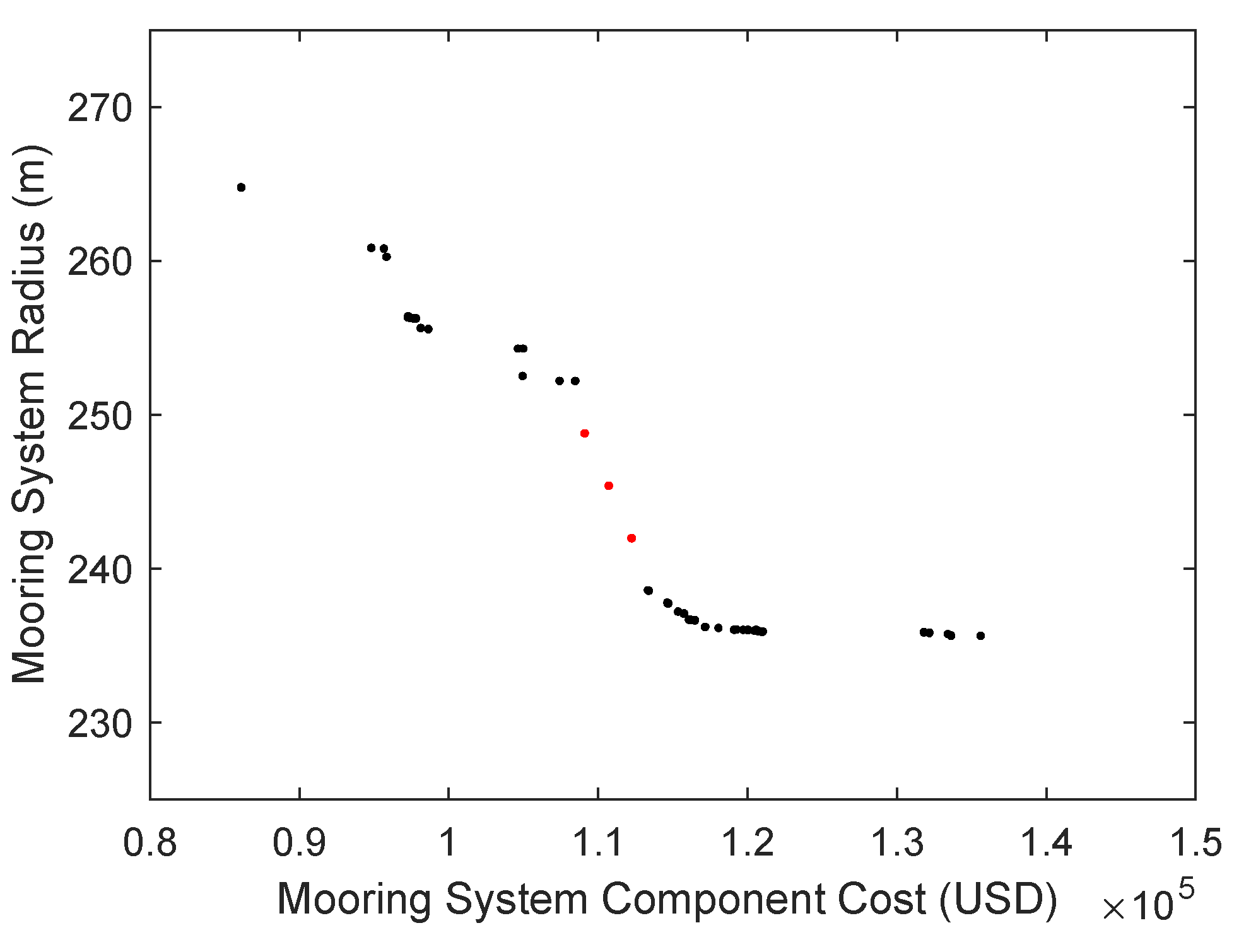
The most interesting aspect of the Pareto-optimal front presented in Figure 10 is the gap in the front from designs jumping from a radius of 252 m to 239 m. To investigate the phenomenon the 252 m radius and 239 m radius designs were used to generate three interpolated designs between them. These three designs where then evaluated for potential constraint violations, which all failed. This suggests that the region between these two feasible designs contains designs that if feasible are dominated by other designs along the Pareto front. The three failed interpolated designs are presented as red dots on the Pareto-optimal front in Figure 14.
To determine what it would take to make one of the interpolated designs feasible the design at a radius of 245 m was analyzed more closely. The synthetic line length varies in a very linear manner as shown in Figure 11 so it was kept the same. The chain and synthetic diameters were then changed from 90% of the interpolated values to 110% of the interpolated values to see how much larger the lines need to be for the mooring system to be a valid solution. The chain diameter and synthetic diameter are scaled by the same amount and the constraint values are recorded. Designs at this interpolated radius and line length become valid after increasing the diameter of the lines by just 3%. Unfortunately, that 3% increase in diameter increases the cost of the mooring system to 116,800 USD or 3% more than the 239 m radius which has a cost of 113,300 USD. As the valid design along the Pareto front has both a smaller mooring footprint and a lower cost when compared to the valid interpolated value the design along the Pareto front will dominate the potential design for a mooring radius of 245 m.

Verification of Candidate Design with Full Suite of DLC 6.1 Simulations

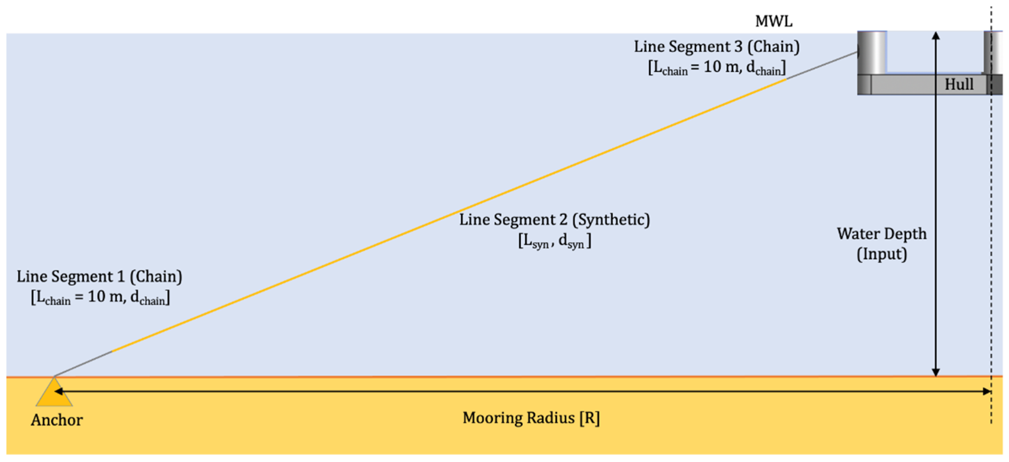
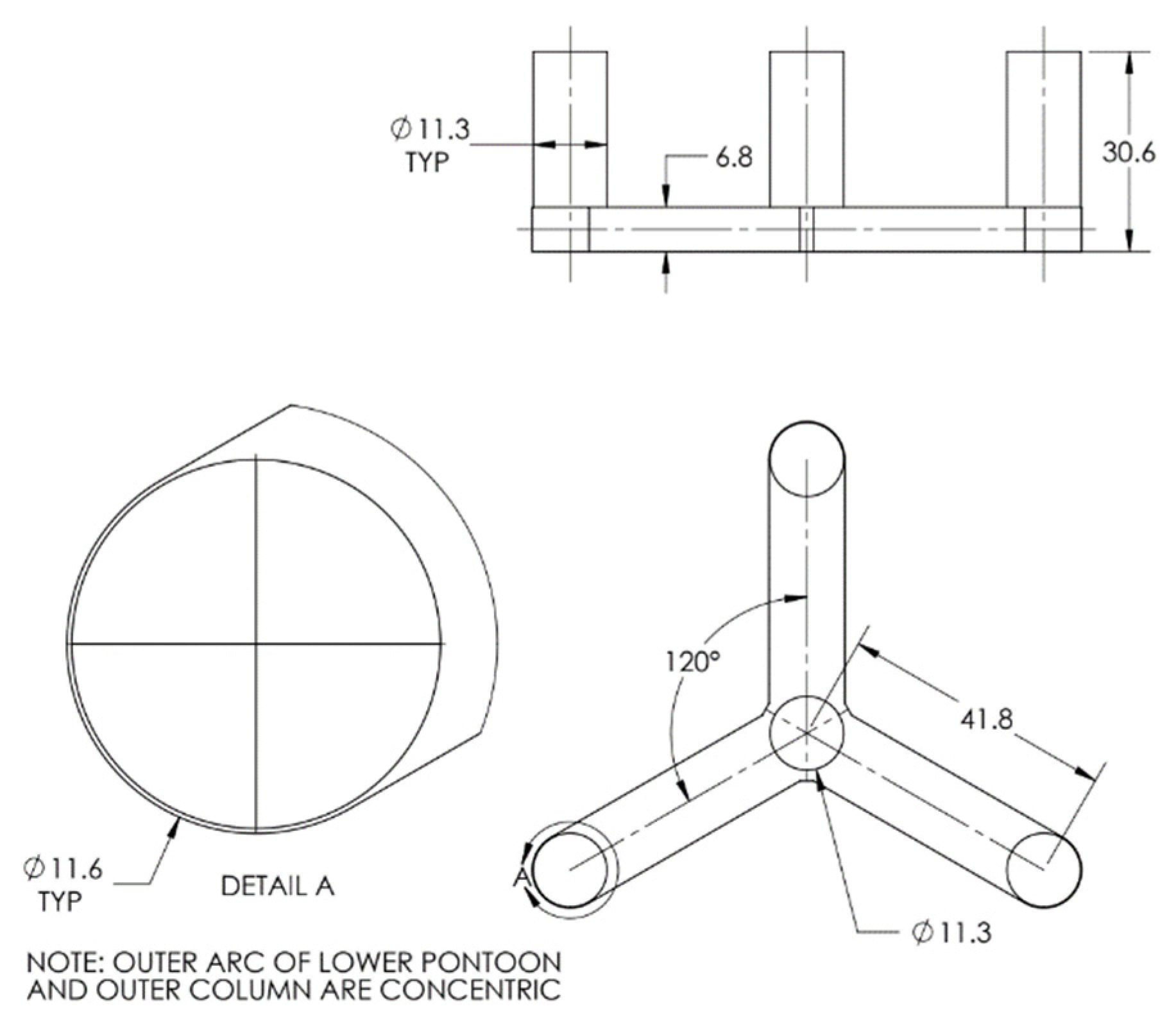
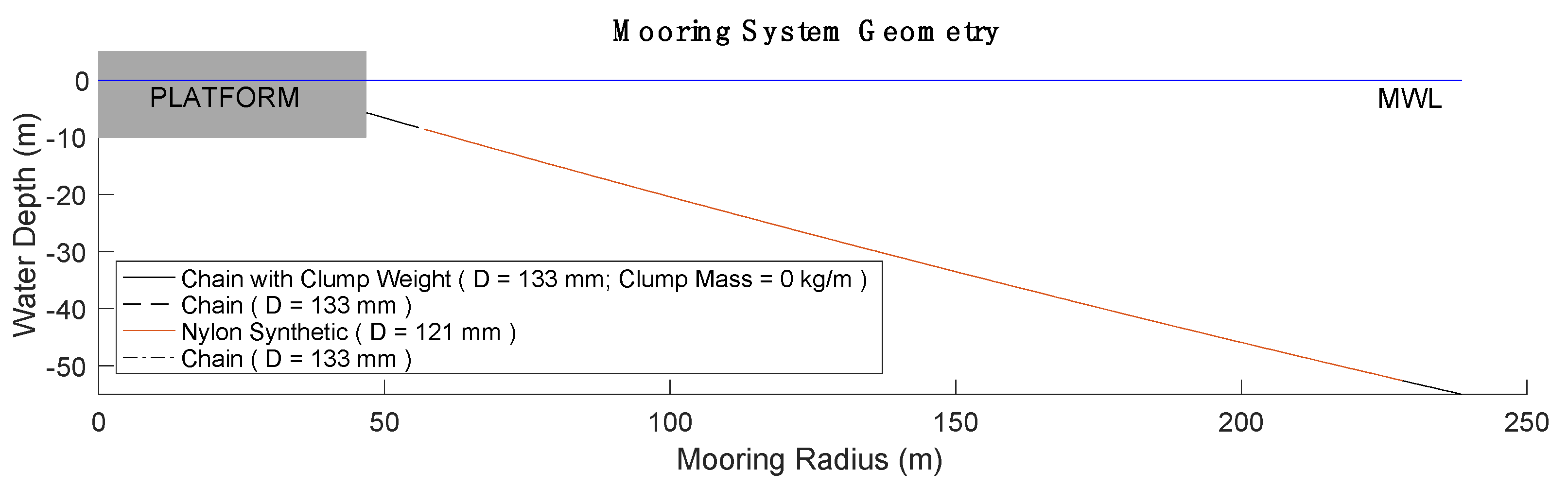
To make the optimization problem computationally feasible performance enhancements such as predicting the maximum design tension based on a shorter simulation time was used in addition to running fairly large timesteps for the simulations. In order to determine if this influenced the Pareto-optimal designs in any way, a full DLC 6.1 suite of simulations was run for one of the candidate designs and the tensions required for evaluating the constraints reexamined. The design picked to be analyzed was a design with a mooring radius of 239 m and a component cost of roughly 113,000 USD. This design was selected as it allowed for the smallest radius design before the mooring line costs begin to increase very drastically. This design has a mooring radius that is 10% smaller than the least expensive design and accomplishes this at a price that is 30% more than the least expensive design. A schematic of the mooring system shown to scale is provided in Figure 15.
The candidate design mooring system is described in Table 10. As outlined in the optimization problem description, this mooring system has three mooring lines spaced equally with each line fairlead connected to one of the outer columns on the VolturnUS 6-MW hull. This mooring system has 10 m of 133 mm diameter chain at the fairlead and anchor with a 167 m long length of 121 mm diameter synthetic spanning between the two chain segments. The fairlead attachments are situated 5.4 m below the water connected to the radius of the outer columns 45.7 m away from the center of the platform.
The results for the DLC 6.1 runs are presented in Table 11. The same seeds were used as presented in 
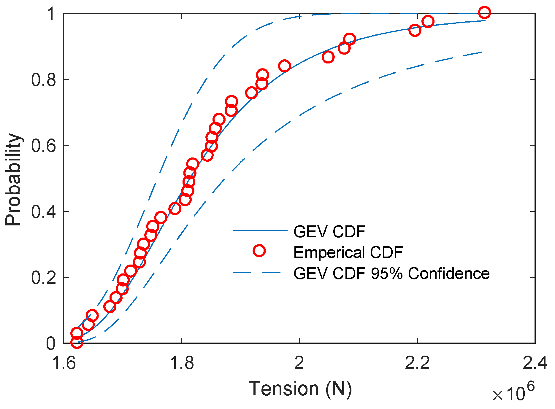
Figure 9 for determining the GEV parameters. The initial run and the statistics are similar when compared to the initial run with the coefficients of variation for the mean tension and the standard deviation of the line being 0.2% and 6.1% respectively. This compares well with the statistics from the trial run of 0.2% and 5.4% for mean tension and standard deviation. The 1000 s extrapolated value for the candidate design using the GEV distribution was 1815 kN which is 1% lower than the ABS design value based on the mean of the maximum tension response value of 1835 kN. Again, this compares very well with the trial run where the GEV extrapolated value was 2% higher than the ABS design value. If proper care is taken to carefully choose a seed and an appropriate statistical fit a shorter simulation can be run to obtain maximum line responses that are close to the ABS design values. It should be noted that this was for one wave orientation, and it is possible that this approach will not work in all cases. However, the results for this one optimization scenario were deemed very acceptable.

6. Conclusions

This paper outlines the effort to implement a MOGA, NSGA II, for design optimization of synthetic mooring systems for FOWTs. The objective functions for this problem are fairly trivial, but a significant time investment was made ensuring the constraints implemented would lead to mooring designs that were realistic and adhered to the ABS/IEC design guidelines. To adequately capture the physics of a mooring system which can experience both geometric and material non-linearities it is imperative that time-domain simulations are run. Time-domain simulations are computationally expensive so the constraints are posed in such a way that inadequate designs can be screened out which prevents running time domain simulations unnecessarily. To make the problem computationally feasible on a normal desktop computer some concessions needed to be made such as reducing the number of simulations done, using fairly large timesteps and carefully selecting seeds which will produce line tensions representative of the true design value.
This method was then used to develop a set of Pareto-optimal designs which balance the footprint of the mooring system and the mooring system component cost. The Pareto-optimal solutions found from this optimization contained a gap in the front which was found to be a result of the designs in that area having constraint violations due to the tensions in the line being slightly too large for the materials load capacity. The lines would handle the load in the lines if both the synthetic and chain segments were increased in diameter by 3% however the cost increase from this resulted in a design that would be dominated by designs having a smaller component cost and radius.
A design that resulted in a small footprint was analyzed more in depth to determine if the 1000 s of data used to extrapolate the maximum tension was adequate. The seed used was carefully chosen based on a DLC 6.1 run for another synthetic mooring system. The candidate design mooring system was then subjected to the same DLC 6.1 simulations with the same seed as the initial analysis of the synthetic mooring system. The value obtained from the 1000 s of extrapolated data was within 2% of the ABS design value found by taking the mean of the maximum values of the six one-hour simulations. Overall, this methodology provides designs that balance mooring line cost and mooring footprint and would be a good starting point for performing a full suite of ABS/IEC simulations.
Ideally, for future work this method would be used without the performance enhancements needed to make it computationally feasible on the hardware available. This would be fairly easy to implement given a computer with more cores available for parallel processing as the computer used in this study was an average desktop computer with four cores. With adequate computational resources the OpenFAST time domain simulations could be run with fully turbulent wind fields for the full 3600 s which at this point is not possible as it would require timesteps that are so small it would make the problem computationally infeasible.
Moving forward there are recommendations for improvements. Most importantly increasing the accuracy of the cost data for evaluating the cost objective function. Currently the only cost considered is the material cost for the chain and synthetic segments, but to deploy a FOWT there are many additional costs that need to be considered including engineering and project management, installation costs and connection costs. Lastly and most importantly from an engineering perspective is the anchoring costs which depend on both soil conditions and loads which would only be known after running the OpenFAST time domain simulations. Factoring in these additional costs would lead to much more realistic estimates moving forward.
It would be interesting to expand this approach to other types of mooring system configurations such as chain catenary or hybrid semi-taut systems. It is not clear if these configurations would be a good candidate for multi-objective optimization as it is unknown if cost and mooring footprint would be competing. These configurations could be good candidates for single objective optimization where the same tiered-constraint methodology proposed by the authors could be implemented to determine the feasibility by screening out designs and avoid running time-domain simulations on infeasible designs.

Author Contributions

Conceptualization, W.W., A.G. and A.V. methodology, W.W., A.G., S.H. and A.V.; software, W.W.; writing—original draft preparation, W.W.; writing—review and editing, A.G. and S.H.; supervision, A.G., S.H. and A.V.; project administration, S.H. and A.V.; funding acquisition, A.G. and A.V.; All authors have read and agreed to the published version of the manuscript.

Funding

This research was funded by the New York State Energy Research and Development Authority (NYSERDA).

Institutional Review Board Statement

Not applicable.

Informed Consent Statement

Not applicable.

Data Availability Statement

Not applicable.

Acknowledgments

Thanks to the Harold Alfond Foundation for Additional Funding.

Conflicts of Interest

The authors declare no conflict of interest.

Abbreviations

ABSAmerican Bureau of Shipping
CDFCumulative distribution function
CMCenter of mass
DLCDesign load case
FOSFactor of safety
FOWTFloating offshore wind turbine
GEVGeneralized extreme value fit
IECInternational Electrotechnical Commission
MAP++Mooring Analysis Program
MBSMinimum breaking strength
MWMegawatt
QTFQuadratic transfer function
SLCSurvival Load Case
SWL/MWLStill water line/Mean water line
UVUltraviolet
a 33 infinite period added mass of the platform in heave
a 55 infinite period added inertia of the platform in pitch
dtMMoorDyn timestep
dtFOpenFAST timestep
d c h a i n chain diameter
d s y n synthetic diameter
Dfdepth from the mean water line (MWL) to the fairlead connection point
D w water depth
F f _ chain chain fatigue factor
F s _ syn synthetic factor of safety for a synthetic
F min _ syn minimum allowable line tension to avoid slack lines as a percentage of MBS
HsSignificant wave height
I platform platform pitch inertia
k 33 platform heave stiffness
k 33 Mooring mooring system heave stiffness
k 55 platform pitch stiffness
k 55 Mooring mooring system pitch stiffness
LMlumped masses the mooring line is discretized into using MoorDyn
L s y n length of synthetic segment (expressed as a fraction of mooring radius)
Lrtotal line length
m platform mass of the platform
MBS chain minimum breaking strength of the chain
MBS syn minimum breaking strength of the synthetic
R mooring radius
R f distance from the center of the platform to the fairlead connection point
T fairlead _ max maximum tension at the fairlead
T n _ heave platform heave natural period
T n _ pitch platform pitch natural period
T syn _ max maximum tension at the fairlead
T syn _ min minimum tension at the fairlead
TpPeak period
γ Peak shape factor

References

  1. US Department of Energy. Offshore Wind Market Report: 2021 Edition; US Department of Energy: Washington, DC, USA, 2021.
  2. Xu, K.; Larsen, K.; Shao, Y.; Zhang, M.; Gao, Z.; Moan, T. Design and comparative analysis of alternative mooring systems for floating wind turbines in shallow water with emphasis on ultimate limit state design. Ocean Eng. 2021, 219, 108377. [Google Scholar] [CrossRef]
  3. Davies, P.; Weller, S.D.; Johanning, L.; Banfield, S.J. A review of synthetic fiber moorings for marine energy applications. In Proceedings of the 5th International Conference on Ocean Energy, Halifax, NS, Canada, 4–6 November 2014; pp. 1–6. [Google Scholar]
  4. Flory, J.F.; Banfield, S.J.; Ridge, I.M.; Yeats, B.; Mackay, T.; Wang, P.; Hunter, T.; Johanning, L.; Herduin, M.; Foxton, P. Mooring systems for marine energy converters. In Proceedings of the OCEANS 2016 MTS/IEEE Monterey, Monterey, CA, USA, 19–23 September 2016; pp. 1–13. [Google Scholar]
  5. Brommundt, M.; Krause, L.; Merz, K.; Muskulus, M. Mooring System Optimization for Floating Wind Turbines using Frequency Domain Analysis. Energy Procedia 2012, 24, 289–296. [Google Scholar] [CrossRef] [Green Version]
  6. Benassai, G.; Campanile, A.; Piscopo, V.; Scamardella, A. Optimization of Mooring Systems for Floating Offshore Wind Turbines. Coast. Eng. J. 2015, 57, 1550021. [Google Scholar] [CrossRef] [Green Version]
  7. Hall, M.; Goupee, A. Validation of a lumped-mass mooring line model with DeepCwind semisubmersible model test data. Ocean Eng. 2015, 104, 590–603. [Google Scholar] [CrossRef] [Green Version]
  8. Thomsen, J.B.; Ferri, F.; Kofoed, J.P.; Black, K. Cost Optimization of Mooring Solutions for Large Floating Wave Energy Converters. Energies 2018, 11, 159. [Google Scholar] [CrossRef] [Green Version]
  9. Pillai, A.C.; Thies, P.R.; Johanning, L. Mooring system design optimization using a surrogate assisted multi-objective genetic algorithm. Eng. Optim. 2019, 51, 1370–1392. [Google Scholar] [CrossRef] [Green Version]
  10. Li, L.; Jiang, Z.; Ong, M.C.; Hu, W. Design optimization of mooring system: An application to a vessel-shaped offshore fish farm. Eng. Struct. 2019, 197, 109363. [Google Scholar] [CrossRef]
  11. Ferreira, F.M.; Lages, E.; Afonso, S.M.B.; Lyra, P.R. Dynamic design optimization of an equivalent truncated mooring system. Ocean Eng. 2016, 122, 186–201. [Google Scholar] [CrossRef]
  12. Deb, K.; Pratap, A.; Agarwal, S.; Meyarivan, T. A Fast and Elitist Multiobjective Genetic Algorithm. IEEE Trans. Evol. Comput. 2002, 6, 182–197. [Google Scholar] [CrossRef] [Green Version]
  13. Goupee, A.J.; Vel, S.S. Multi-objective optimization of functionally graded materials with temperature-dependent material properties. Mater. Des. 2007, 28, 1861–1879. [Google Scholar] [CrossRef]
  14. West, W. Design and Modelling of Synthetic Mooring Systems for Floating Offshore Wind Turbines. Master’s Thesis, University of Maine, Orono, ME, USA, 2019. [Google Scholar]
  15. Masciola, M. MAP ++ Documentation. 2018. Available online: https://map-plus-plus.readthedocs.io/_/downloads/en/latest/pdf/ (accessed on 1 October 2021).
  16. Hall, M. MoorDyn User’s Guide; University of Maine: Orono, ME, USA, 2015. [Google Scholar]
  17. NREL. OpenFAST Documentation Release v2.3.0; National Renewable Energy Laboratory: Golden, CO, USA, 2020.
  18. West, W.M.; Goupee, A.J.; Allen, C.; Viselli, A.M. Floating Wind Turbine Model Test to Verify a MoorDyn Modification for Nonlinear Elastic Materials. J. Offshore Mech. Arct. Eng. 2021, 1–41. [Google Scholar] [CrossRef]
  19. WAMIT. WAMIT R User Manual. 2020. Available online: https://www.wamit.com/manualupdate/v74_manual.pdf (accessed on 1 October 2021).
  20. IEC. IEC 61400-3 Design Requirements for Offshore Wind Turbines; IEC: Geneve, Switzerland, 2019. [Google Scholar]
  21. ABS. Guide for Building and Classing Floating Offshore Wind Turbine Installations; ABS: Spring, TX, USA, 2015. [Google Scholar]
  22. ABS. Guidance Notes on the Application of Fiber Rope for Offshore Mooring; ABS: Spring, TX, USA, 2014. [Google Scholar]
  23. ABS. Guide for Position Mooring Systems; ABS: Spring, TX, USA, 2020. [Google Scholar]
  24. Weller, S.D.; Johanning, L.; Davies, P.; Banfield, S.J. Synthetic mooring ropes for marine renewable energy applications. Renew. Energy 2015, 83, 1268–1278. [Google Scholar] [CrossRef] [Green Version]
  25. API. API RP 2SM: Recommended Practice for Design, Manufacture, Installation, and Maintenance of Synthetic Fiber Ropes for Offshore Mooring; API: Washington, DC, USA, 2014. [Google Scholar]
  26. ABS. ABS Review Advances University of Maine’s Innovative Floating Offshore Wind Concept; ABS: Spring, TX, USA, 2017. [Google Scholar]
  27. Viselli, A.M.; Forristall, G.Z.; Pearce, B.R.; Dagher, H.J. Estimation of extreme wave and wind design parameters for offshore wind turbines in the Gulf of Maine using a POT method. Ocean Eng. 2015, 104, 649–658. [Google Scholar] [CrossRef] [Green Version]
  28. Dagher, H.; Viselli, A.; Goupee, A.; Kimball, R.; Allen, C. The VolturnUS 1:8 Floating Wind Turbine: Design, Construction, Deployment, Testing, Retrieval, and Inspection of the First Grid-Connected Offshore Wind Turbine in US; University of Maine: Orono, ME, USA, 2017. [Google Scholar]
  29. Allen, C.; Viselli, A.; Dagher, H.; Goupee, A.; Gaertner, A.; Abbas, N.; Hall, M.; Barter, G. Definition of the UMaine VolturnUS-S Reference Platform Developed for the IEA Wind 15-Megawatt Offshore Reference Wind Turbine; NREL/TP-5000-76773; National Renewable Energy Laboratory: Golden, CO, USA, 2020. Available online: https://www.nrel.gov/docs/fy20osti/76773.pdf (accessed on 23 November 2021).
  30. DNV. Global Perfomance Analysis of Deepwater Floating Structures; DNV: Bærum, Norway, 2004. [Google Scholar]
Figure 1. NSGA II Flowchart.
Modelling 02 00039 g001
Figure 2. Constraint and Objective Calculation Flow Chart.
Modelling 02 00039 g002
Figure 3. Geometric Feasibility Design Constraint.
Modelling 02 00039 g003
Figure 4. Mooring System Schematic for Optimization.
Modelling 02 00039 g004
Figure 5. Material Tension-Strain Relationships.
Modelling 02 00039 g005
Figure 6. Dry Chain Mass and Chain Load Capacity (left) and Dry Synthetic Mass and Synthetic Load Capacity (right).
Modelling 02 00039 g006
Figure 7. VolturnUS 6-MW Platform Dimensions in Meters.
Modelling 02 00039 g007
Figure 8. Example Fairlead Tension Cumulative Distribution Function.
Modelling 02 00039 g008
Figure 9. OpenFAST and MoorDyn Time Step Convergence Study.
Modelling 02 00039 g009
Figure 10. Designs along the Pareto-Optimal Front.
Modelling 02 00039 g010
Figure 11. Mooring System Radius vs. Synthetic Line Length.
Modelling 02 00039 g011
Figure 12. Mooring Radius vs. Chain Diameter for Designs on the Pareto-optimal Front.
Modelling 02 00039 g012
Figure 13. Mooring Radius vs. Synthetic Diameter for Designs along the Pareto-optimal Front.
Modelling 02 00039 g013
Figure 14. Designs along the Pareto-Optimal Front (black) with Interpolated Designs with Constraint Violations (red).
Modelling 02 00039 g014
Figure 15. Illustration of the Optimized Candidate Design for the VolturnUS 6-MW Turbine.
Modelling 02 00039 g015
Table 1. Mooring System Properties.
Number of mooring lines3
Angle of mooring lines (0° aligned with positive surge axis; positive defined as counter-clockwise)60°, 180°, 300°
Depth to anchors below SWL (water depth)55 m
Depth to fairleads below SWL5.4 m
Radius to anchors from platform centerlineDesign Variable
Radius to fairleads from platform centerline45.7 m
Unstretched chain length (Leader)10 m
Unstretched chain length (Anchor)10 m
Unstretched synthetic lengthDesign Variable
Synthetic line diameterDesign Variable
Chain diameterDesign Variable
Table 2. Mooring System Material Costs.
MaterialCost (USD/kg)
Steel1.50
Synthetic17.00
Table 3. FOWT Component Mass and Locations.
Total Draft20.0 m
Platform Mass, Including Ballast1.09 × 107 kg
Displacement1.17 × 104 m3
Center of Mass (CM) Location Below SWL Along Platform Centerline11.85 m
Platform Roll Inertia About CM5.23 × 109 kg-m2
Platform Pitch Inertia About CM5.23 × 109 kg-m2
Platform Yaw Inertia About CM8.33 × 109 kg-m2
Hub Height Above SWL100 m
Total Tower Top Mass557,000 kg
Tower Mass246,000 kg
Tower CM above SWL72.9 m
Table 4. Mooring System Design Requirements.
Synthetic Minimum Breaking Factor of Safety2.18
Chain Minimum Breaking Factor of Safety6.78
Partial safety factor for DLC 6.1 Loads1.35
Minimum Line Tension2% of Synthetic MBS
Minimum Platform Surge Period40 s
Minimum Platform Heave Period18 s
Minimum Platform Pitch Period25 s
Table 5. FOWT Environmental Loading.
Wave Loading
JONSWAP SpectrumHs (m)Tp (s)γ
10.714.22.75
Mean Load due to Second-order Wave EffectsMean Load (kN)
19.9
Current Loading
Mean Load due to CurrentCurrent Velocity (m/s)Mean Load (kN)
0.2849
Wind Loading
Mean Load due to WindWind Velocity (m/s)Mean load (kN)
23.8290
Table 6. DLC 6.1 Results for VolturnUS 6-MW Moored with a Basin Tested 6-MW System (0 Degree Loading; Front Line).
HydroDyn SEED 1HydroDyn SEED 2Max Tension (N)Min Tension (N)Mean Tension (N)STD Tension (N)
674,802,239−228,621,0852.36 × 1062.78 × 1051.13 × 1063.44 × 105
−2,090,187,7751,455,391,3022.92 × 1062.27 × 1051.13 × 1063.63 × 105
−1,973,081,278−629,542,9152.59 × 1062.59 × 1051.13 × 1063.67 × 105
301,302,578−328,425,0232.82 × 1061.33 × 1051.13 × 1063.88 × 105
81,611,327265,255,7962.48 × 1062.52 × 1051.13 × 1063.38 × 105
133,186,3421,154,134,0953.31 × 1061.75 × 1051.13 × 1063.82 × 105
Table 7. Extrapolating the Maximum 1-Hour DLC 6.1 Line Tensions using 1000 s of Simulation Data.
RunNumber of Peaks in 1000 sNumber of Peaks Extrapolated to 3600 sProbability of Maximum Tension in 3600 sPredicted Tension (N)
A4616599.39%2.81 × 10⁶
B4516299.38%3.97 × 10⁶
C4616599.39%3.18 × 10⁶
D4415899.36%3.67 × 10⁶
E4516299.38%2.44 × 10⁶
F5118399.45%2.17 × 10⁶
Table 8. OpenFAST and MoorDyn Convergence Study.
10 Lumped Masses40 Lumped Masses160 Lumped Masses
OpenFAST Timesteps (s)MoorDyn Timesteps (ms)OpenFAST Timesteps (s)MoorDyn Timesteps (ms)OpenFAST Timesteps (s)MoorDyn Timesteps (ms)
0.252.50.252.50.11.0
0.1750.1750.075
0.1251.250.1251.250.050.5
0.0750.0750.025
0.0250.250.0250.250.010.1
0.00250.00250.001
Table 9. OpenFAST and MoorDyn Convergence Study.
Converged ValueValue for dtM = 2.5 ms; dtF = 0.175 s; LM = 10Percent Difference (%)
Max Fair Tension1273 kN1308 kN2.7
Max Syn Tension1274 kN1263 kN−0.9
Min Syn Tension353 kN343 kN−2.8
Max Anch Tension1271 kN1253 kN−1.4
Max Surge Displacement9.89 m9.79 m−1.0
Max Pitch Displacement
(From Resting Position) *
0.52 deg0.46 deg−1.9
* Mean Pitch displacement is −2.54 degrees.
Table 10. VolturnUS 6-MW Optimized Candidate Design.
Number of mooring lines3
Angle of mooring lines (0° aligned with positive surge axis)60°, 180°, 300°
Depth to anchors below SWL (water depth)55 m
Depth to fairleads below SWL5.4 m
Radius to anchors from platform centerline239 m
Radius to fairleads from platform centerline45.7 m
Unstretched chain length (Leader)10 m
Unstretched chain length (Anchor)10 m
Unstretched synthetic length167 m
Synthetic line diameter121 mm
Chain diameter133 mm
Component Cost113,310 USD
Table 11. DLC 6.1 Results for VolturnUS 6-MW Moored with the Optimized Candidate Design.
SEED 1SEED 2Max Tension (N)Min Tension (N)Mean Tension (N)STD Tension (N)
674,802,239−228,621,0851.63 × 1063.32 × 1059.46 × 1051.86 × 105
−2,090,187,7751,455,391,3021.97 × 1063.29 × 1059.47 × 1051.98 × 105
−1,973,081,278−629,542,9151.74 × 1063.50 × 1059.45 × 1052.01 × 105
301,302,578−328,425,0231.79 × 1062.30 × 1059.45 × 1052.14 × 105
81,611,327265,255,7961.69 × 1063.30 × 1059.43 × 1051.85 × 105
133,186,3421,154,134,0952.16 × 1062.80 × 1059.47 × 1052.11 × 105
Publisher’s Note: MDPI stays neutral with regard to jurisdictional claims in published maps and institutional affiliations.

