
Characterizing Prediction Uncertainty in Agricultural Modeling via a Coupled Statistical–Physical Framework


Abstract
:1. Introduction
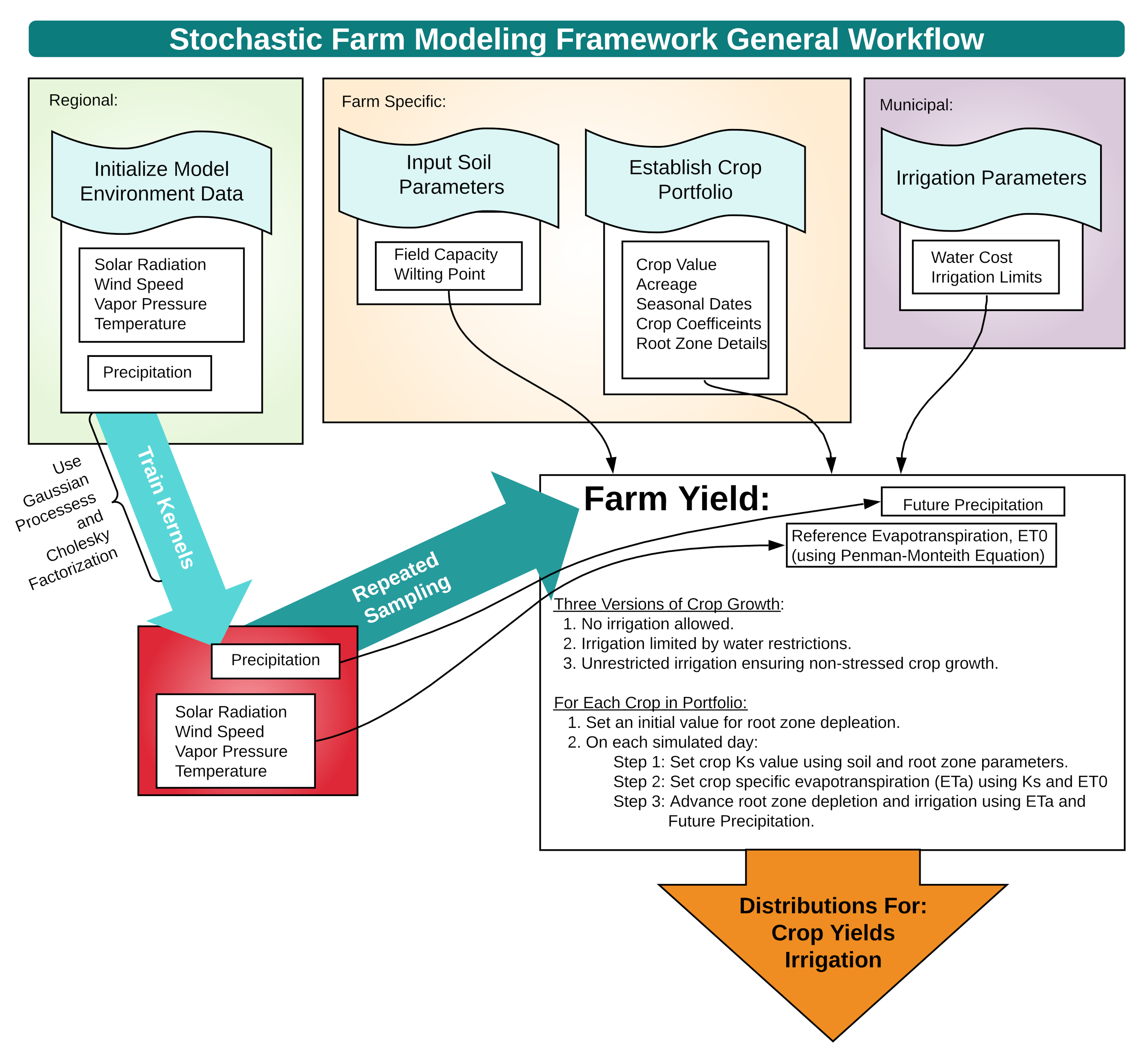
2. Physical Model
2.1. Modeling Evapotranspiration
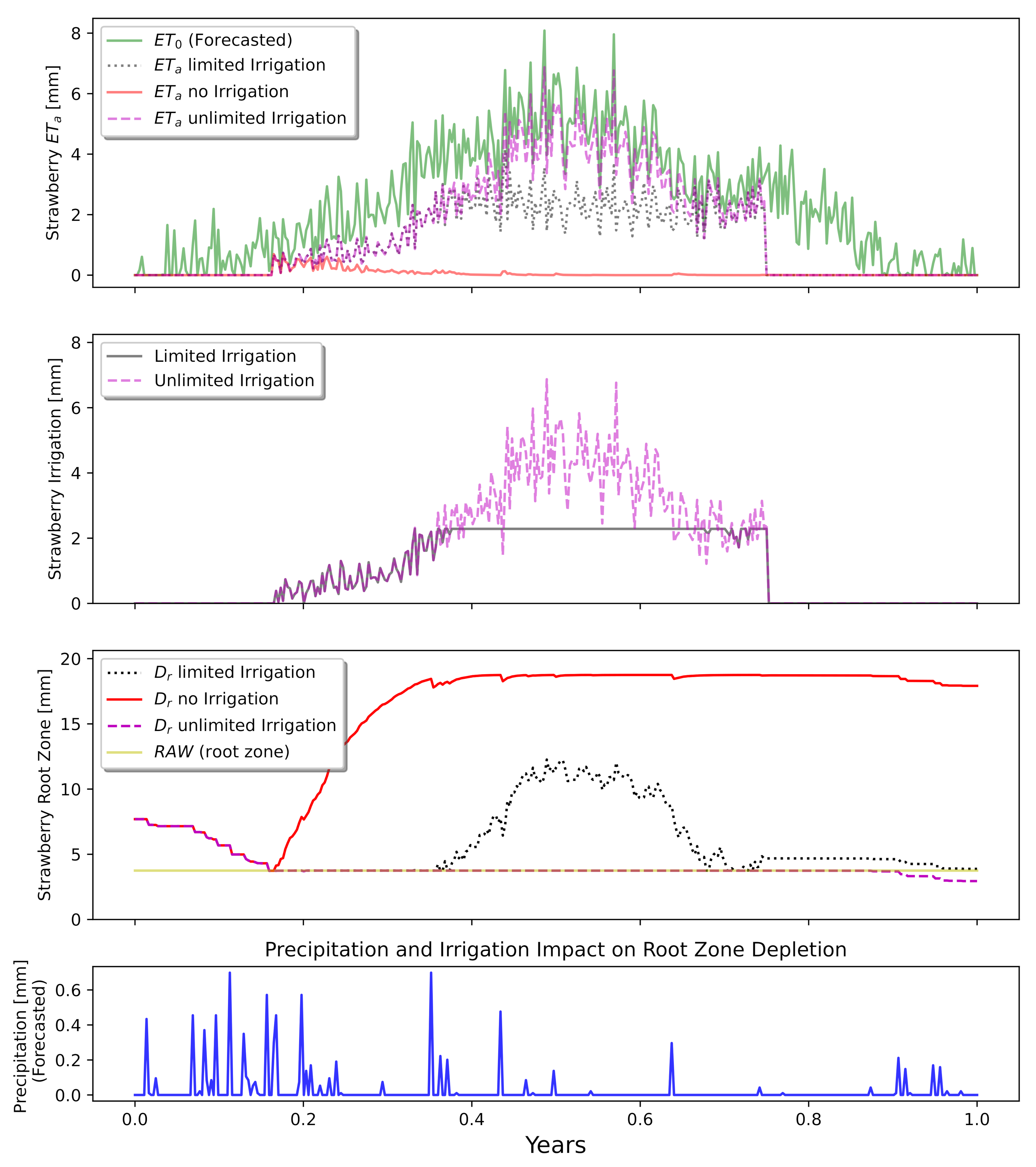
2.2. Modeling Soil Water Availability
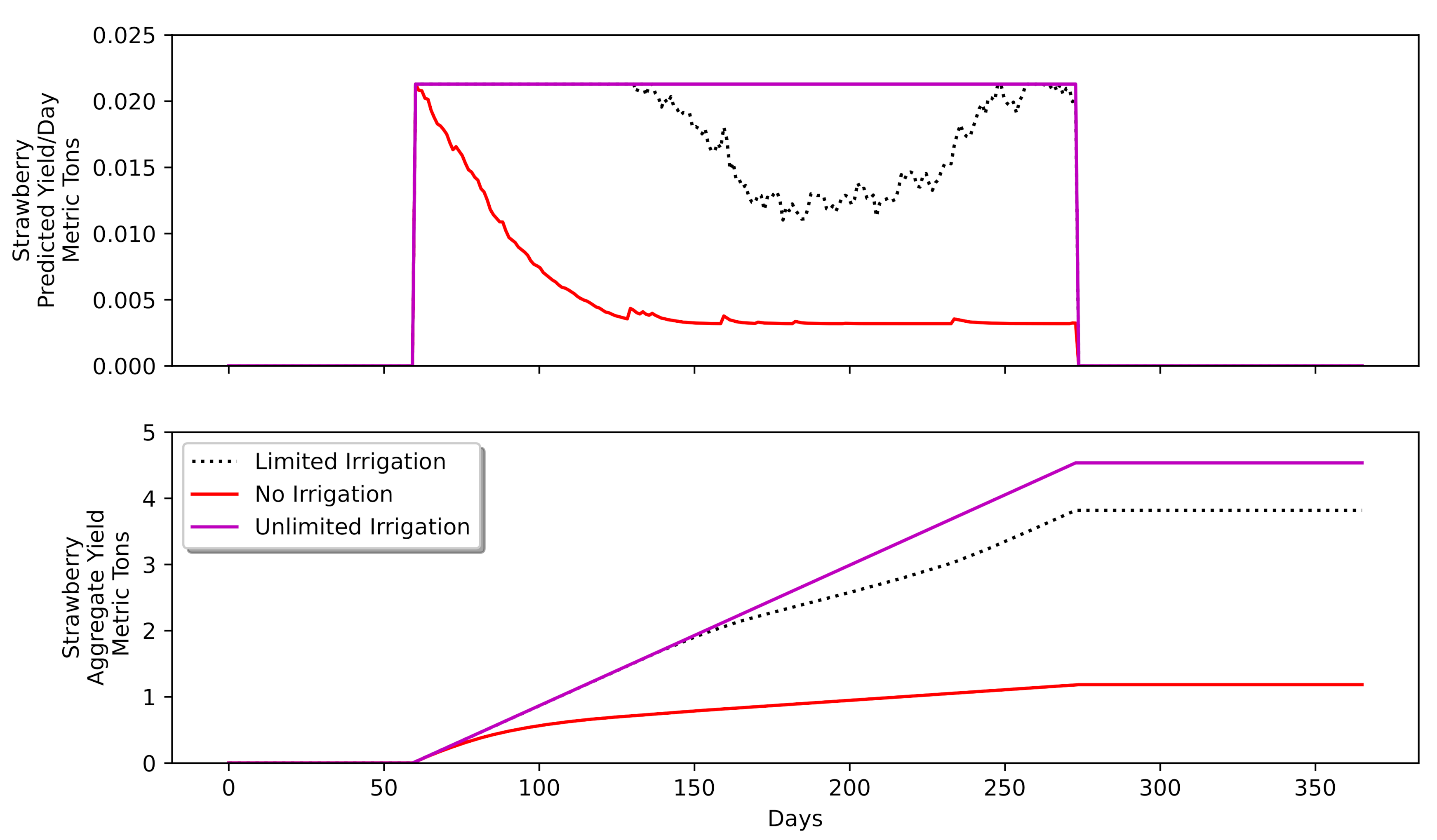
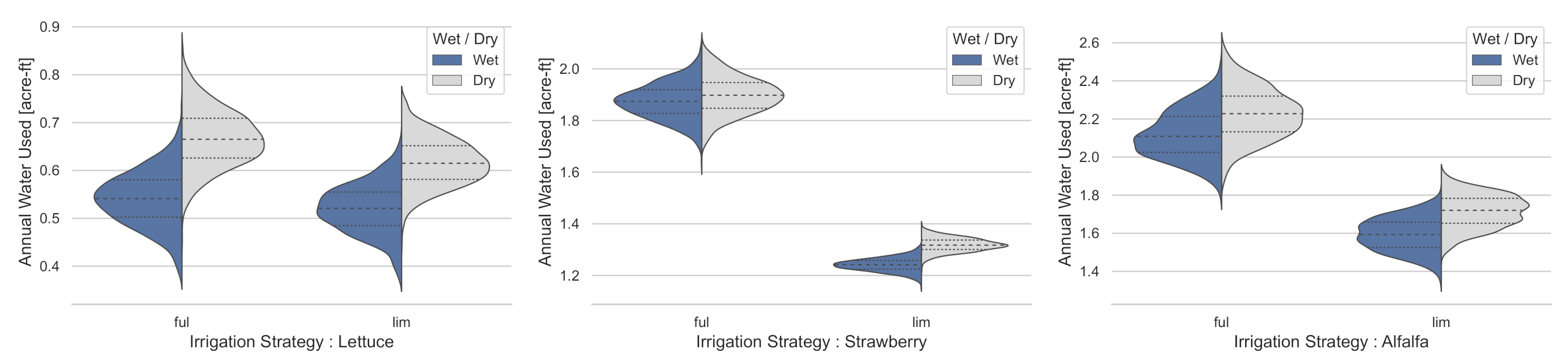
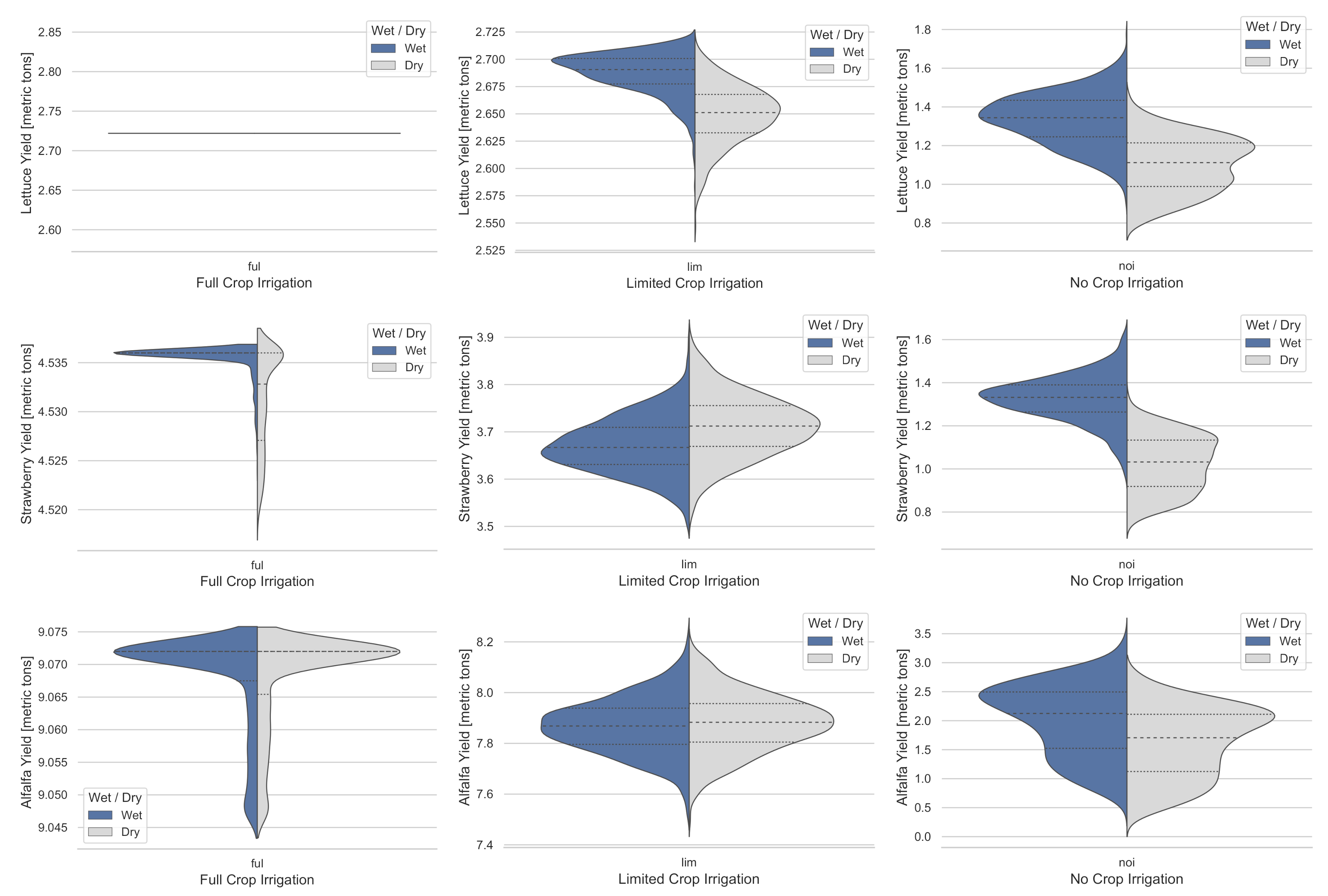
2.3. Strategies for Irrigation
3. Statistical Characterization of the Environment
3.1. Gaussian Process Background
3.1.1. RBF Kernel
3.1.2. Matern Kernel
3.1.3. Periodic Matern Kernel
3.1.4. Constant Kernel
3.1.5. White Noise Kernel
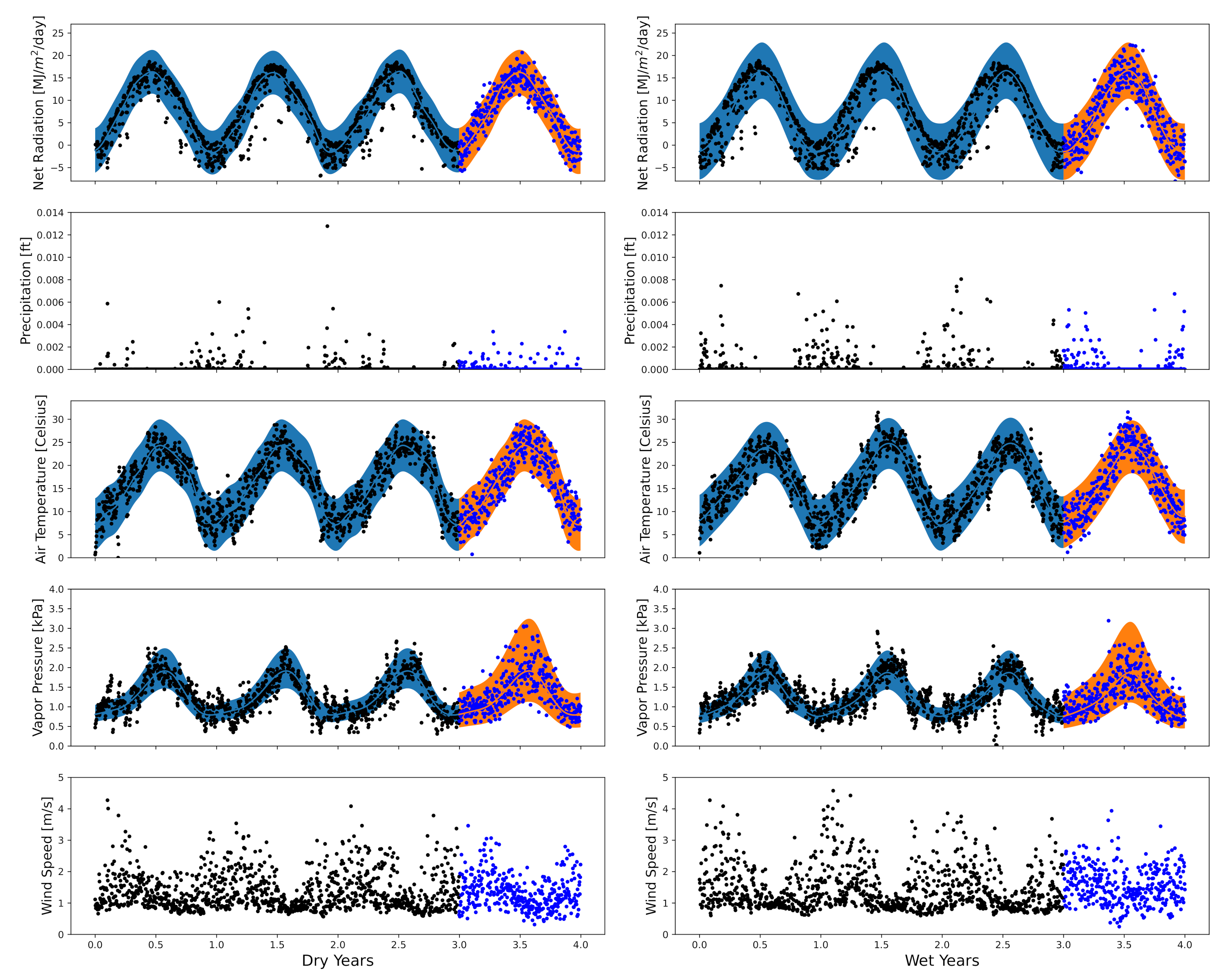
3.2. Stochastic Process Models for Environmental Parameters
3.2.1. Temperature
3.2.2. Net Radiation
3.2.3. Atmospheric Pressure

3.2.4. Modeling Precipitation
3.2.5. Modeling Wind Speed
4. Numerical Results


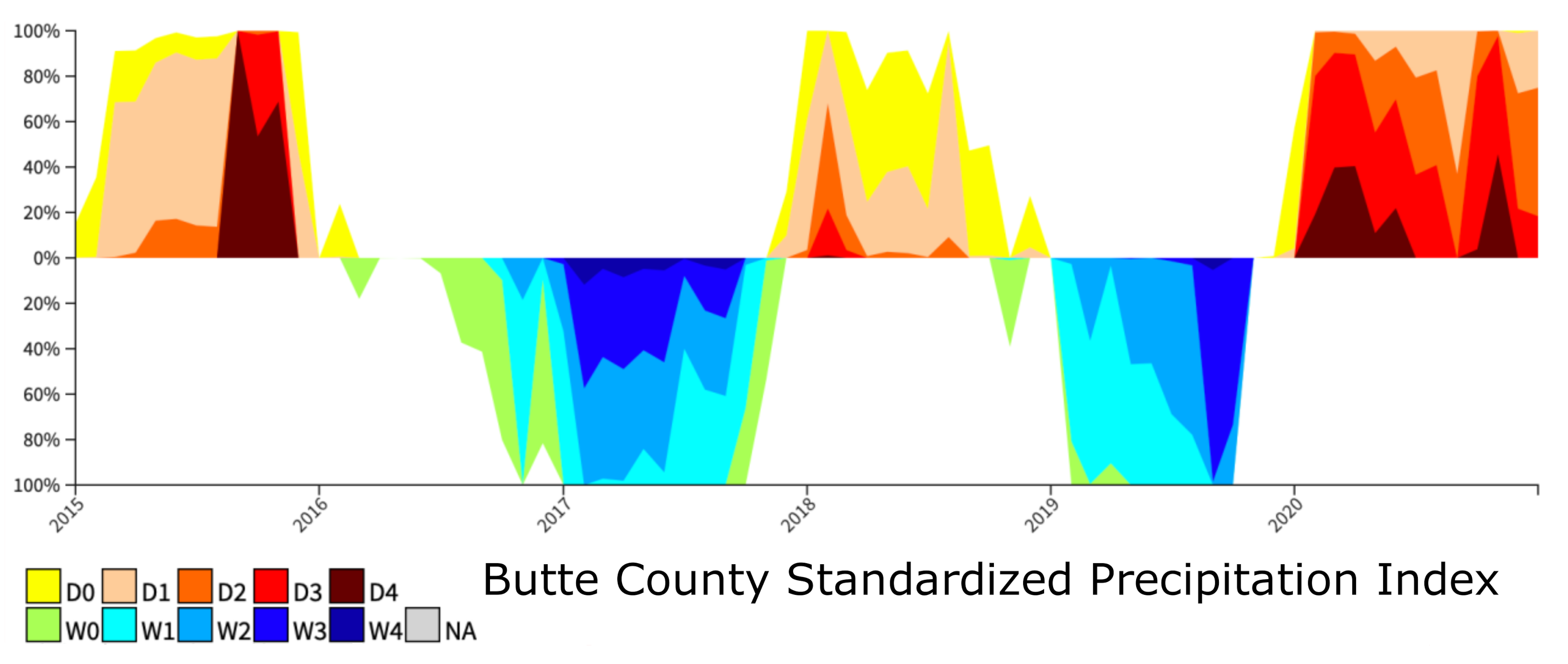
4.1. Classification of Forecasting Data
4.2. Example Farming Environment
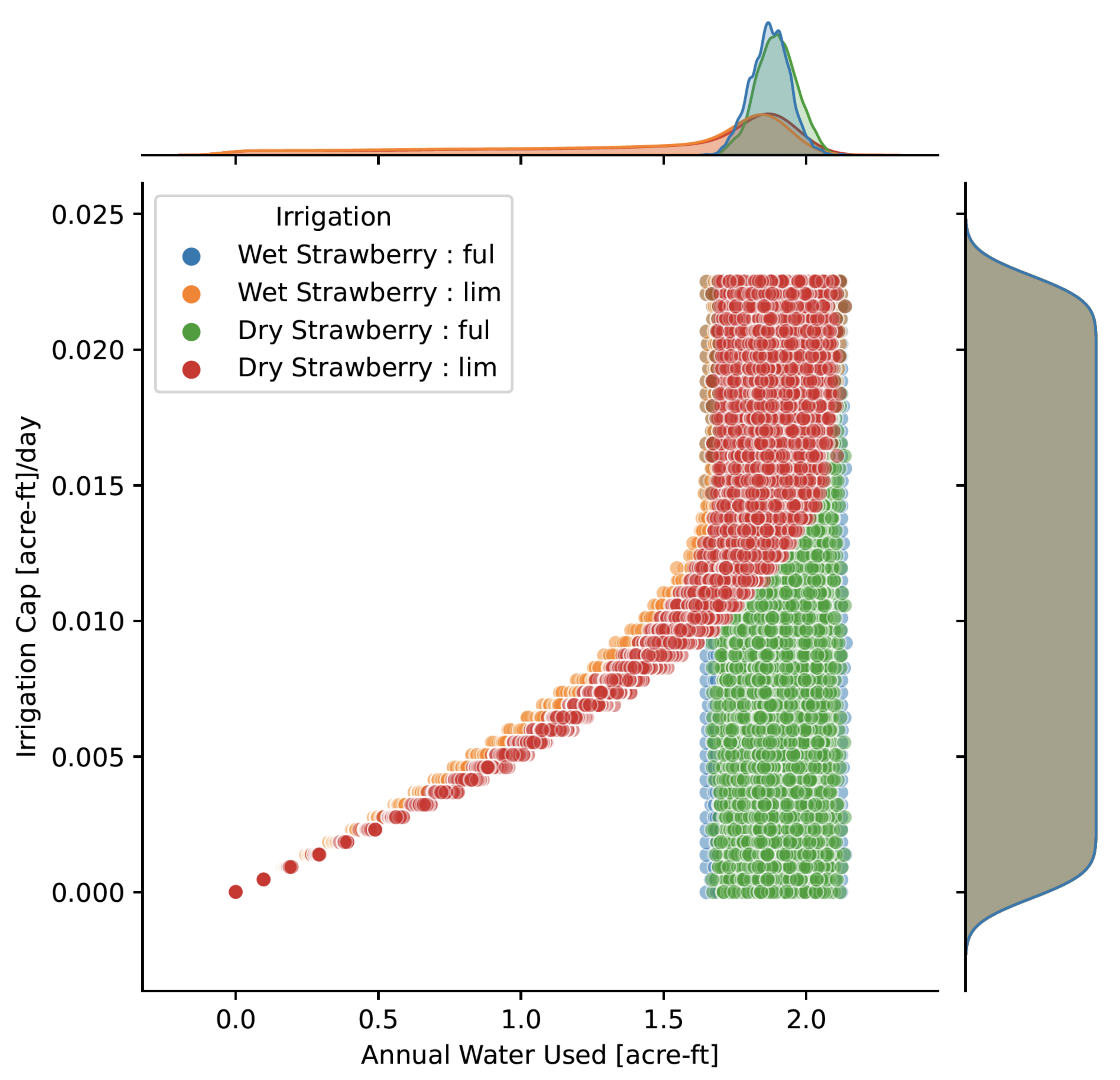
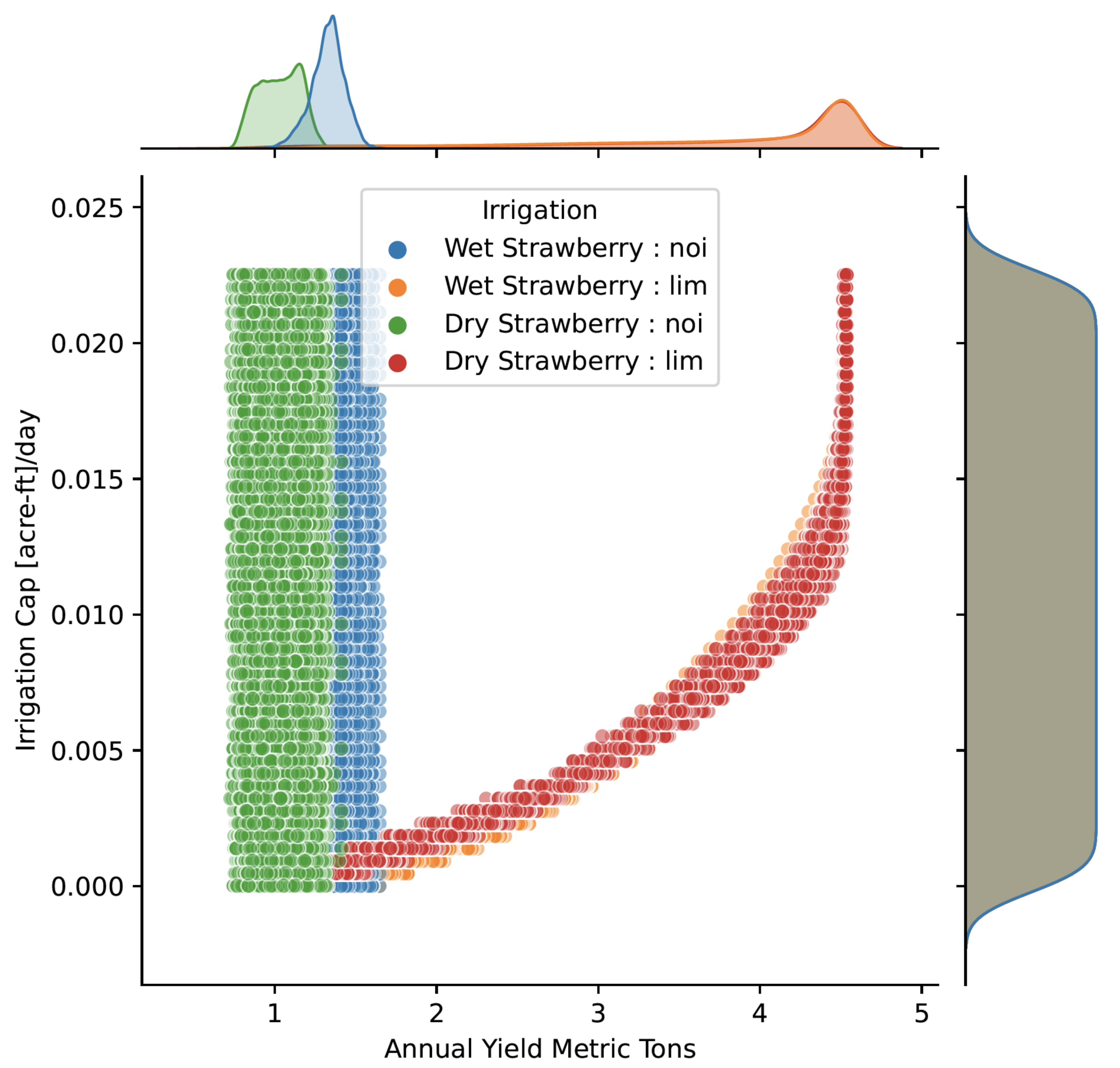
4.3. Varying Limits on Water Use
5. Global Sensitivity Analysis
5.1. Background
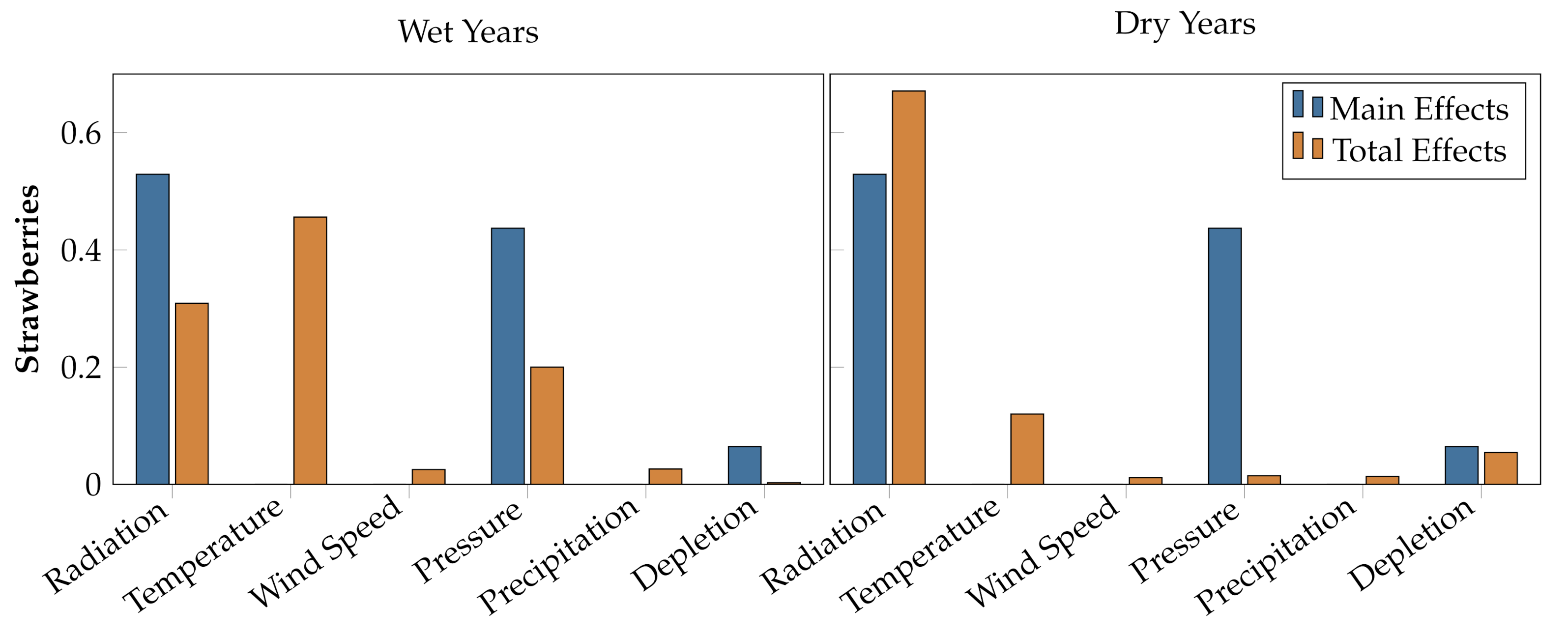
5.2. Sensitivity Results
6. Conclusions and Future Directions
Author Contributions
Funding
Conflicts of Interest
References
- De Clercq, M.; Vats, A.; Biel, A. Agriculture 4.0: The future of farming technology. In Proceedings of the World Government Summit, Dubai, United Arab Emirates, 11–13 February 2018. [Google Scholar]
- NOAA. Global Climate Indicators. Available online: https://www.climate.gov/news-features/understanding-climate/global-climate-indicators (accessed on 9 December 2021).
- Gray, E. NASA at Your Table: Climate Change and Its Environmental Impacts on Crop Growth. NASA Earth Science News, 1 September 2021. Available online: https://www.nasa.gov/feature/goddard/esnt/2021/nasa-at-your-table-climate-change-and-its-environmental-impacts-on-crop-growth(accessed on 8 December 2021).
- Tropp, D.; Moraghan, M. Local food demand in the U.S.: Evolution of the marketplace and future potential. In Harvesting Opportunity: The Power of Regional Food System Investments to Transform Communities; Dumont, A., Davis, D., Wascalus, J., Wilson, T., Barham, J., Tropp, D., Eds.; Federal Reserve Bank of St. Louis, the Board of Governors of the Federal Reserve System: St. Louis, MO, USA, 2017; pp. 15–42. [Google Scholar]
- Tropp, D. From anecdote to formal evaluation: Reflections from more than two decades on the local food research trail at USDA. J. Agric. Food Syst. Community Dev. 2019, 9, 13–30. [Google Scholar] [CrossRef] [Green Version]
- Robinson, J.; Farmer, J. Selling Local: Why Local Food Movements Matter; Indiana University Press: Bloomington, IN, USA, 2017. [Google Scholar]
- Shelef, O.; Fernández-Bayoand, J.; Sher, Y.; Ancona, V.; Slinn, H.; Achmon, Y. Elucidating local food production to identify the principles and challenges of sustainable agriculture. In Sustainable Food Systems from Agriculture to Industry; Elsevier: London, UK, 2018; pp. 47–81. [Google Scholar]
- Kriewald, S.; Pradhan, P.; Costa, L.; Ros, A.G.C.; Kropp, J.P. Hungry cities: How local food self-sufficiency relates to climate change, diets, and urbanisation. Environ. Res. Lett. 2019, 14, 094007. [Google Scholar] [CrossRef]
- Thilmany, D.; Canales, E.; Low, S.; Boys, K. Local Food Supply Chain Dynamics and Resilience during COVID-19. Appl. Econ. Perspect. Policy 2021, 43, 86–104. [Google Scholar] [CrossRef]
- Udias, A.; Pastori, M.; Dondeynaz, C.; Carmona Moreno, C.; Abdou, A.; Cattaneo, L.; Cano, J. A decision support tool to enhance agricultural growth in the Mékrou river basin (West Africa). Comput. Electron. Agric. 2018, 154, 467–481. [Google Scholar] [CrossRef]
- Zhai, Z.; Martínez, J.F.; Beltran, V.; Martínez, N. Decision support systems for agriculture 4.0: Survey and challenges. Comput. Electron. Agric. 2020, 170, 105256. [Google Scholar] [CrossRef]
- Bronson, K. The Digital Divide and How it Matters for Canadian Food System Equity. Can. J. Commun. 2019, 44, 63–68. [Google Scholar] [CrossRef] [Green Version]
- Chrispell, J.; Fowler, K.; Howington, S.; Jenkins, E.; Minik, M.; Sendova, T. Mathematical modeling, simulation, and optimal design for agricultural water management. In Proceedings of the 2012 SC Water Resources Conference, Columbia, SC, USA, 10–11 October 2012. [Google Scholar]
- Bokhiria, J.; Fowler, K.; Jenkins, E. Modelling and optimization for crop portfolio management under limited irrigation strategies. J. Agric. Environ. Sci. 2014, 3, 209–237. [Google Scholar]
- Fowler, K.; Jenkins, E.; Ostrove, C.; Chrispell, J.; Farthing, M.; Parno, M. A decision making framework with MODFLOW-FMP2 via optimization: Determining trade-offs in crop selection. Environ. Model. Softw. 2015, 69, 280–291. [Google Scholar] [CrossRef] [Green Version]
- Fowler, K.; Jenkins, E.; Parno, M.; Chrispell, J.; Colón, A.; Hanson, R. Development and use of mathematical models and software frameworks for integrated analysis of agricultural systems and associated water use impact. AIMS Agric. Food 2016, 1, 208–226. [Google Scholar] [CrossRef]
- Steduto, P.; Hsiao, T.; Fereres, E.; Raes, D. Crop Yield Response to Water. FAO Irrigation and Drainage; Technical Report 66; Food and Agriculture Organization of the United Nations: Rome, Italy, 2012. [Google Scholar]
- Allen, R.; Pereira, L.; Raes, D.; Smith, M. Crop Evapotranspiration Guidelines for Computing Crop Water Requirements FAO 56; Technical Report 56; Food and Agriculture Organization of the United Nations: Rome, Italy, 1998. [Google Scholar]
- Cornell University Cooperative Extension. (Fact Sheet 29) Agronomy Fact Sheet Series: Soil Texture. Available online: http://nmsp.cals.cornell.edu/publications/factsheets/factsheet29.pdf (accessed on 9 December 2021).
- California Department of Water Resources. California Irrigation Management Information Systems. Available online: https://cimis.water.ca.gov/ (accessed on 9 December 2021).
- GPy. GPy: A Gaussian Process Framework in Python. 2012. Available online: http://github.com/SheffieldML/GPy (accessed on 9 December 2021).
- Durrande, N.; Hensman, J.; Rattray, M.; Lawrence, N.D. Gaussian process models for periodicity detection. PeerJ Comput. Sci. 2016, 2, 1–18. [Google Scholar] [CrossRef] [Green Version]
- Williams, C.K.; Rasmussen, C.E. Gaussian Processes for Machine Learning; MIT Press: Cambridge, MA, USA, 2006. [Google Scholar]
- Kleiber, W.; Katz, R.W.; Rajagopalan, B. Daily spatiotemporal precipitation simulation using latent and transformed Gaussian processes. Water Resour. Res. 2012, 48, W01523. [Google Scholar] [CrossRef] [Green Version]
- U.S. Government. National Integrated Drought Information System. Available online: https://www.drought.gov/states/california/county/butte (accessed on 9 December 2021).
- Saltelli, A.; Annoni, P.; Azzini, I.; Campolongo, F.; Ratto, M.; Tarantola, S. Variance based sensitivity analysis of model output. Design and estimator for the total sensitivity index. Comput. Phys. Commun. 2010, 181, 259–270. [Google Scholar] [CrossRef]
- Hanson, R.T.; Boyce, S.E.; Schmid, W.; Hughes, J.D.; Mehl, S.W.; Leake, S.A.; Maddock, T., III; Niswonger, R.G. One-Water Hydrologic Flow Model (MODFLOW-OWHM); Technical Report; US Geological Survey: San Diego, CA, USA, 2014.


| Variable | Definition |
|---|---|
| Reference evapotranspiration [mm day] | |
| Net radiation at the crop surface [MJ m d] | |
| atmospheric pressure [kPa] | |
| G | Soil heat flux density [MJ m d] |
| T | Mean daily air temperature at 2 m height [C] |
| Wind speed at 2 m height [m s] | |
| Saturation vapor pressure [kPa] | |
| Actual vapor pressure [kPa] | |
| Slope vapor pressure curve [kPa C] | |
| Psychrometric constant [kPa C] |
| Crop | [m] | p | ||||||
|---|---|---|---|---|---|---|---|---|
| Alfalfa | 1.1 | 9.072 | 0.4 | 0.95 | 0.9 | 1.0 | 0.55 | (0, 365) |
| Lettuce | 1.0 | 2.722 | 0.0 | 1.0 | 0.95 | 0.4 | 0.3 | (15, 120), (258, 349) |
| Strawberry | 0.85 | 4.536 | 0.4 | 0.85 | 0.75 | 0.25 | 0.2 | (60, 273) |
| Crop | Net Radiation | Temperature | Wind Speed | Pressure | Precipitation | Depletion | |
|---|---|---|---|---|---|---|---|
| Wet | Alfalfa | 5.32 | 4.73 | 0.00 | 3.44 | 4.81 | 3.44 |
| Lettuce | 0.00 | 4.08 | 2.94 | 0.00 | 4.14 | 6.62 | |
| Strawberries | 5.29 | 0.00 | 0.00 | 4.37 | 0.00 | 6.45 | |
| Dry | Alfalfa | 0.00 | 7.24 | 0.00 | 9.17 | 0.00 | 1.36 |
| Lettuce | 0.00 | 0.00 | 0.00 | 1.47 | 0.00 | 0.00 | |
| Strawberries | 4.22 | 2.02 | 0.00 | 3.86 | 0.00 | 6.42 |
| Crop | Net Radiation | Temperature | Wind Speed | Pressure | Precipitation | Depletion | |
|---|---|---|---|---|---|---|---|
| Wet | Alfalfa | 2.81 | 3.86 | 2.31 | 1.90 | 2.63 | 1.18 |
| Lettuce | 3.60 | 4.30 | 3.19 | 2.60 | 6.14 | 1.94 | |
| Strawberries | 3.09 | 4.56 | 2.53 | 2.00 | 2.63 | 2.79 | |
| Dry | Alfalfa | 6.10 | 1.27 | 1.37 | 1.62 | 1.10 | 1.16 |
| Lettuce | 5.55 | 2.28 | 3.16 | 2.38 | 1.40 | 7.26 | |
| Strawberries | 6.71 | 1.20 | 1.16 | 1.48 | 1.35 | 5.43 |
Publisher’s Note: MDPI stays neutral with regard to jurisdictional claims in published maps and institutional affiliations. |
© 2021 by the authors. Licensee MDPI, Basel, Switzerland. This article is an open access article distributed under the terms and conditions of the Creative Commons Attribution (CC BY) license (https://creativecommons.org/licenses/by/4.0/).
Share and Cite
Chrispell, J.C.; Jenkins, E.W.; Kavanagh, K.R.; Parno, M.D. Characterizing Prediction Uncertainty in Agricultural Modeling via a Coupled Statistical–Physical Framework. Modelling 2021, 2, 753-775. https://doi.org/10.3390/modelling2040040
Chrispell JC, Jenkins EW, Kavanagh KR, Parno MD. Characterizing Prediction Uncertainty in Agricultural Modeling via a Coupled Statistical–Physical Framework. Modelling. 2021; 2(4):753-775. https://doi.org/10.3390/modelling2040040
Chicago/Turabian StyleChrispell, John C., Eleanor W. Jenkins, Kathleen R. Kavanagh, and Matthew D. Parno. 2021. "Characterizing Prediction Uncertainty in Agricultural Modeling via a Coupled Statistical–Physical Framework" Modelling 2, no. 4: 753-775. https://doi.org/10.3390/modelling2040040
APA StyleChrispell, J. C., Jenkins, E. W., Kavanagh, K. R., & Parno, M. D. (2021). Characterizing Prediction Uncertainty in Agricultural Modeling via a Coupled Statistical–Physical Framework. Modelling, 2(4), 753-775. https://doi.org/10.3390/modelling2040040