1. Introduction
Conventional thermal food processing methods have been described as the simplest and most effective way of preventing food spoilage [
1]. These conventional methods deliver safe food products and extend shelf-life [
2]. The most common conventional heating methods for food processing require heat energy to be generated externally and then transferred to food samples. Typically, this is delivered through convection, radiation, or conduction heating, and these conventional methods often use excessive heat processing that leads to the degradation of the outer portion of food substance, especially when the food substance is of a large size ratio [
3]. Furthermore, the efficiency of the heat transfer mechanisms is limited by the rate of heat transfer from an external medium to the food and by the thermal conductivity of the food itself, which often results in over-processing due to the lengthy processing time required to reach the target temperature, thus creating unwanted temperature peaks and producing poor product quality [
4].
Ohmic heating (OH) is a moderate electric field (MEF) processing technique in which the applied electric field is ≤1 k V/cm, considerably lower than the field strength used in the high voltage pulsed electric fields technology (PEF) [
5]. OH involves the passing of electric current through food products. Heat is generated within the food substance and directly dissipated in the medium with a high efficiency (>90%) via the Joule effect, eliminating the heat-transfer step from the surroundings to the medium by means of temperature gradients or hot surfaces [
6]. Singh and Heldman [
7] explained that the collision of ions within the food substance creates resistance to their movement and increases their kinetic energy, thereby producing heat. As a result, heat is instantly and volumetrically generated within the food substance, due to the ionic motion [
8].
Gavahian and Farahnaky [
9] described the conventional heat treatment methods of radiation, convection, and conduction as the most common but time-consuming and energy-wasting food processing techniques. These inefficiencies in conventional heating methods may present cold spots within food, leading to non-uniform heating or overheated food samples and consequential burning. It was highlighted in [
10] that these inefficiencies are significant in foods containing particulates and in highly viscous foods. In contrast, Ohmic heating volumetrically heats up food samples, so rapid heating is achieved with high efficiency [
5]. Cappato explained in [
11] that food material acts as a resistor in an Ohmic process and directly and quickly converts electrical energy into thermal energy, shortening the heating time.
Other heating methods, apart from conventional heating methods, include microwave heating (MH) and inductive heating (IH). For MH, the heat within the food molecule is generated by the agitation of water molecules within the food [
12]. Therefore, for MH heating, the food substance must contain water molecules. IH in food processing is non-contact, so the heat generated from the ferromagnetic containing vessel is transferred to the food substance by conduction. The heat generated from IH is achieved when current is generated as a result of magnetic field across a ferromagnetic conductor, resulting in a Joule effect [
13].
Other authors modelled the MEF process using different techniques. For example, in [
14], it was shown that the rate of Ohmic heating was directly proportional to the square of the electric field strength and electrical conductivity; therefore, the electrical conductivity could be modelled as a linear function of temperature. In [
15], series and parallel impedance and resistance components were applied to predict the electrical conductivities of foods. The electrical conductivity was estimated from the geometry of the electrodes and the resistance. The gap in the current literature is identified as the lack of instant model validation using experimental data.
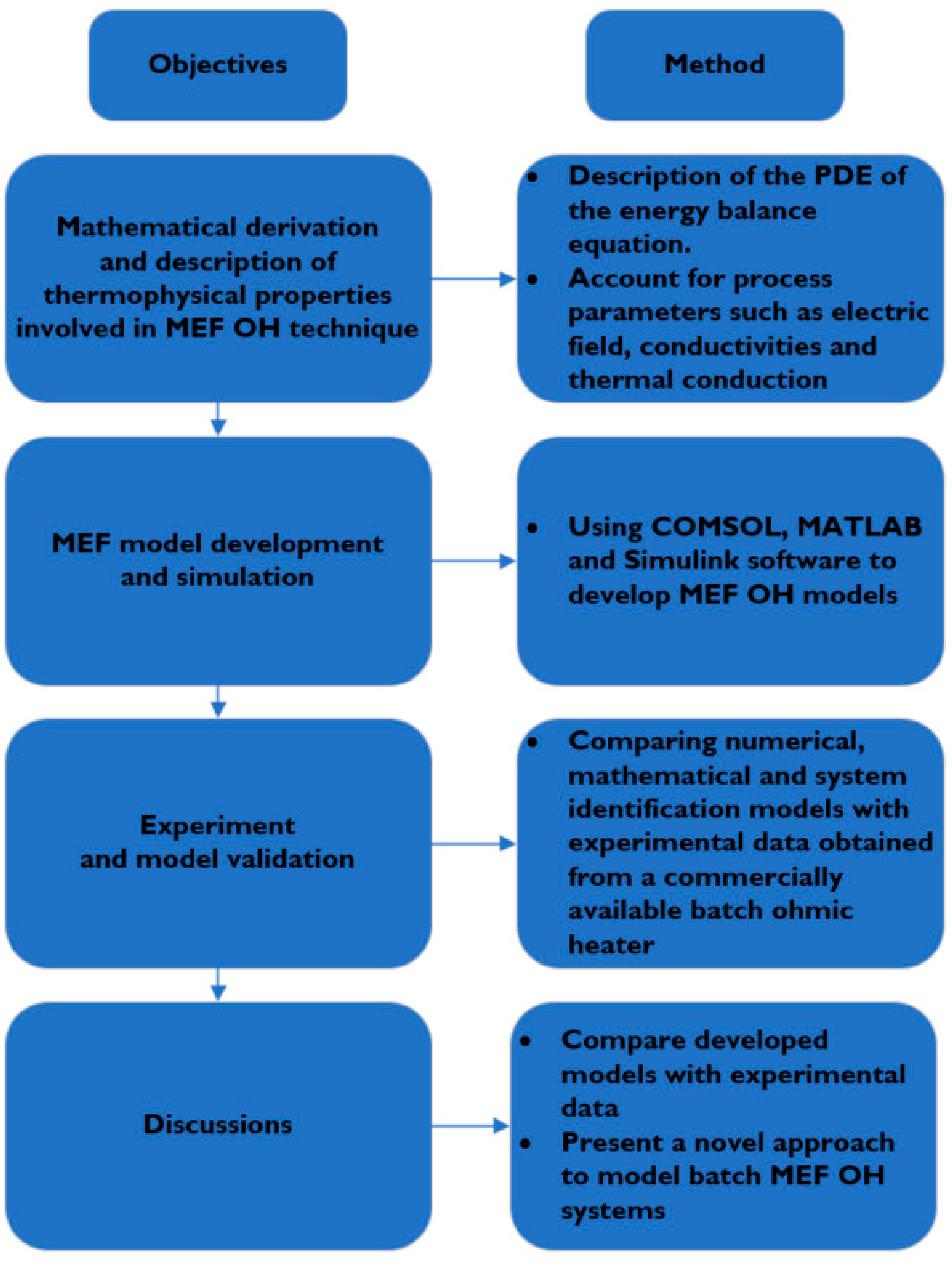
This paper is therefore focused on the dynamic modelling and validation of MEF in food processing and was aimed to address the gap in the literature as follows:
Model the predicted temperature output of different foods under the MEF heating process with variable process parameters.
Present a range of modelling techniques, illustrate their advantages and disadvantages, and validate the simulated models using experimental data.
Compare MEF processes with other alternative emerging processing methods.
3. Ohmic Heating Modelling
3.1. Modelling of the Ohmic Heating Process
During modelling, the temperature of the food substance must be known to ascertain the efficiency of the OH process. Considering a continuous flow OH system, a wide range of thermo–physical properties including fluid flow dynamics, viscosity, density, and mass flow rate interact, thus making it difficult to accurately predict temperature. Therefore, a suitable OH model requires simultaneous solutions of the thermal differential equation, the electrical equation, and fluid flow in the spatial geometry of the OH cell. If a batch OH system is considered, the developed model represents a static thermal system. Therefore, the solution for fluid flow dynamics is ignored, thereby reducing the complexity to only the coupled electrical and thermal partial differential equations (PDE) to enable the determination of the temperature distribution in the OH cell.
3.2. Modelling the General Energy Transfer
The temperature was our primary objective, so the energy transfer equation needed to be solved. The governing equations of the OH system consist of the thermal and electrical equations. Marcotte [
16] presented the thermal conduction and internal energy generation equations as:
where
is the volumetric heat (W/
) generated by the applied electric field (E); T is the temperature term in K;
is the initial temperature; and k, ρ, c, and
are the temperature-dependent thermophysical properties of the food—the thermal conductivity (W/mK), the density (kg/
), the specific heat capacity (J/kg K), and the electrical conductivity (S/m), respectively.
In Equation (1), ∇·(k·∇T) represents the heat transferred by conduction through the fluid, and
represents the volumetric heat generation, which is important in Ohmic heating but negligible in conventional heating processes. The predicted temperature is described by Equation (3) as a function of the conductivity (
), where
is the temperature coefficient (1/K). The fourth term (ρ∇·v) in Equation (1) is the work done by the fluid on its surrounding, which is 0 for an incompressible fluid. The fifth term (
) represents the radiative heat transfer [
16].
The simultaneous solution of the general heat transfer yields:
- -
The equation describing the electrical potential within the food product.
- -
The heat balance equation relating to the electric potential within the food.
- -
The electrical conductivity relating to the temperature.
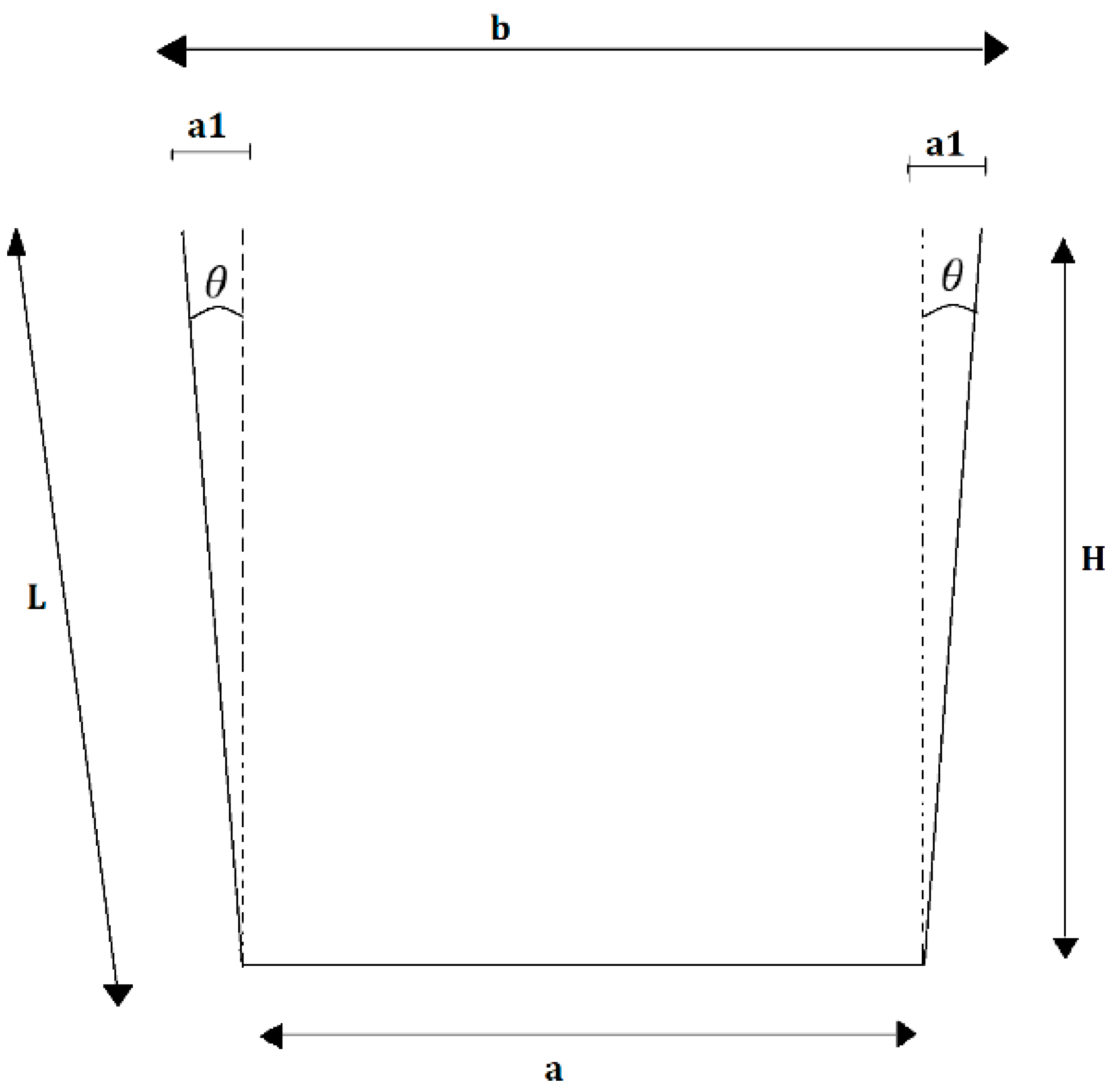
In
Figure 2, the electric field
is modelled as follows:
Assume the electric field is given as:
where
a1 = Lsin
for 0 ≤
.
When = 0, = .
3.3. Model Simulation
General model simulations can be based on three levels of spatial details upon which models of materials can be organized. The microscopic level is concerned to the properties and arrangement of large numbers of atoms and molecules as a crystal structure. The macroscopic level deals with the overall structure averages and is the domain of mechanics and thermodynamics. The mesoscopic level is intermediate to the other two. The macroscopic level requires that the materials’ properties are generally represented by a set of partial differential equations that express energy, mass, and momentum conservation and are formulated to represent the symmetry of the material to which they are applied [
17].
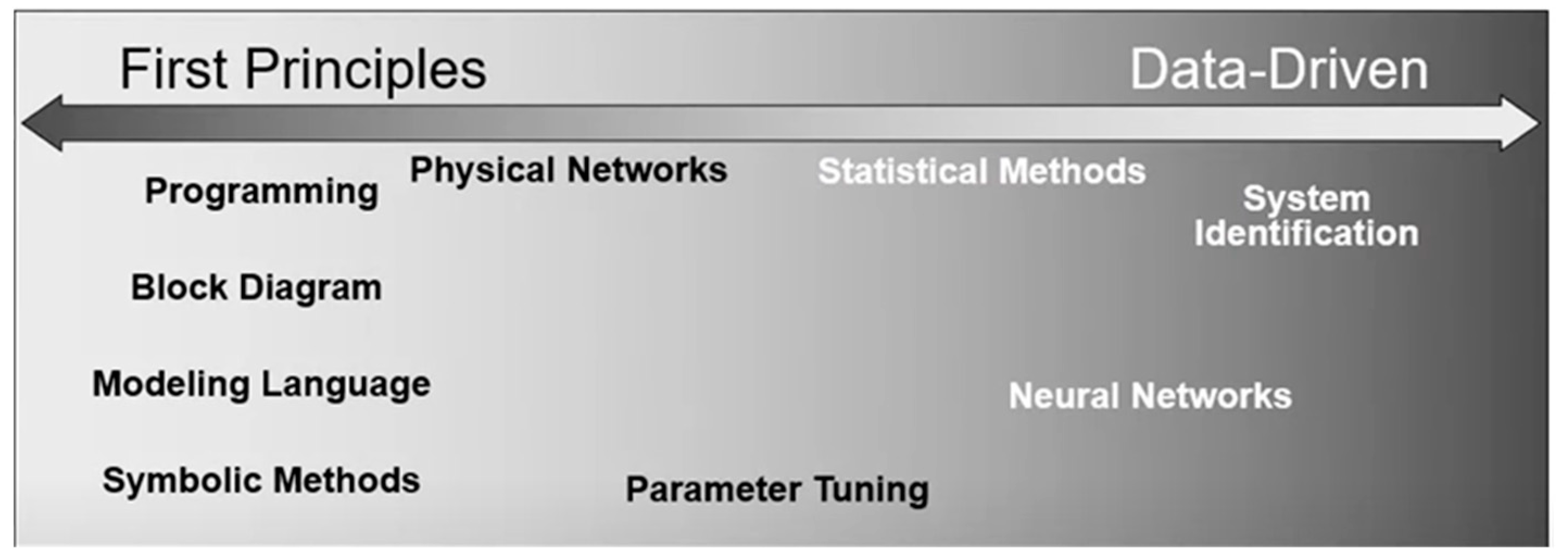
Regarding MEF as an Ohmic heating technique, there is no sharp boundary between the macroscopic and mesoscopic levels. Different food types have varying process parameters (conductivities, viscosity, density, heat capacity, etc.), and these process parameters nonlinearly respond to factors such as applied electric field or initial temperature. Therefore, the modelling approach applied the first principle to the data-driven model techniques as shown in
Figure 3 below Ghosh et al. [
18] described the first-principles or mechanistic modelling as the type of modelling where explicit knowledge of the process mechanism is present and utilized. In this type of modelling, the developed models invoke fundamental physical and chemical laws that describe the system being considered or use partial differential equations. In comparison, the data-driven modelling approach involves mathematical equations that are derived not from physical processes in the catchment but from analyses of time series data [
19].
The Ohmic heating system model is developed using three techniques. These techniques are:
- -
Numerical modelling (Using COMSOL).
- -
Mathematical modelling (block diagram using SIMULINK).
- -
Modelling using system identification technique (Using MATLAB).
The energy balance heat equation of the MEF process is the same for both the numerical and mathematical models. However, the mathematical model provides an analytic method to its solution. The mathematical model uses Simulink blocks that do not follow any defined algorithm but solve the balance equation in a closed form described by the individual blocks; this provides a fast and exact solution [
20], unlike the numerical model, where a robust solution using the backward differential formula (BDF) algorithm is used. However numerical modelling increases computation requirements.
3.3.1. Numerical Modelling
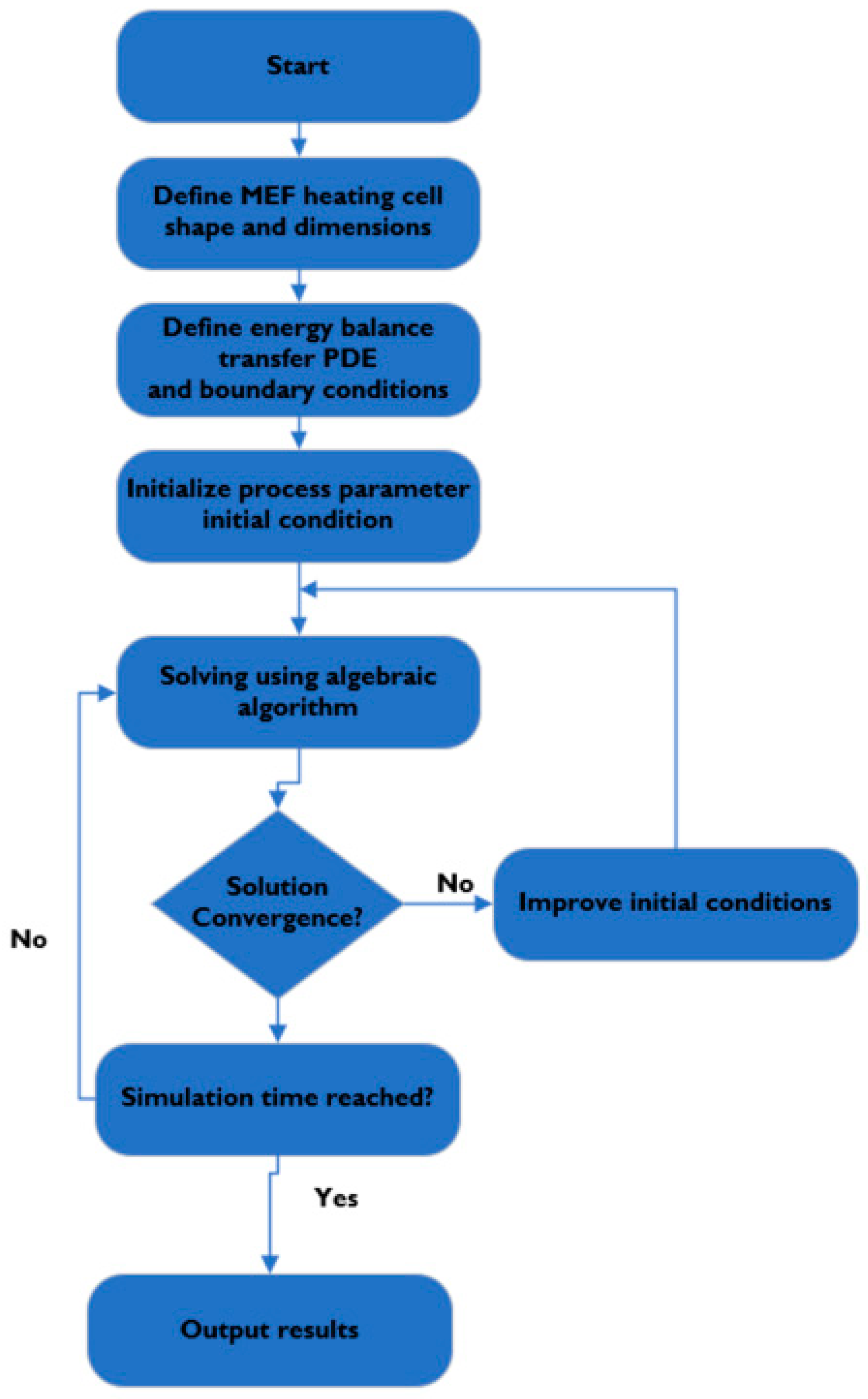
The governing equation, Ohmic heater dimensions, and initial conditions were solved using COMSOL Multiphysics version 5.6 and the electromagnetic heating module (emh). The analysis ran on a PC with Intel core i5 8th Gen CPU at 2.3 GHz with 4 Gb RAM, 8 processors, and the Windows 10 operating system. The electromagnetic heating coupled the electric current (ec) system and the heat transfer (ht) in a solid system into one equation describing the time-dependent equation problem, given in Equation (1). A BDF solver using a time-stepping scheme was used to solve the time-dependent problem for 5108 degrees of freedom (including 2560 internal DOFs). The maximum time constraint was set to automatic such that at each time step, the software could need to solve a set of nonlinear equations. Where a nonlinear system was encountered, the BDF method event tolerance was set to 0.001. An arbitrary linear system solver was then used for the final solution. A flowchart showing the general procedure for the numerical modelling and solving of PDEs is presented in
Figure 4.
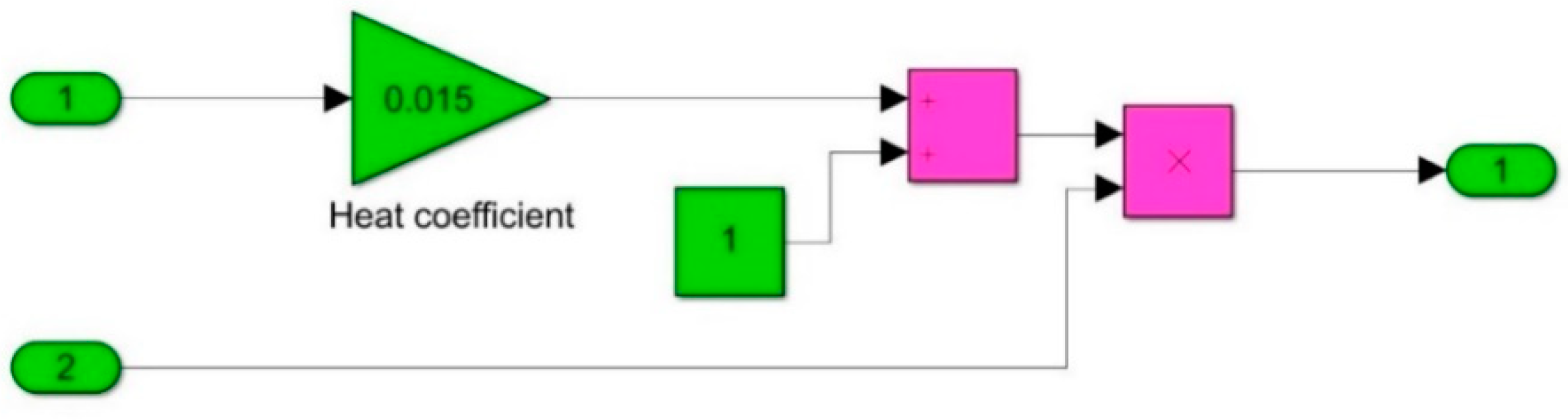
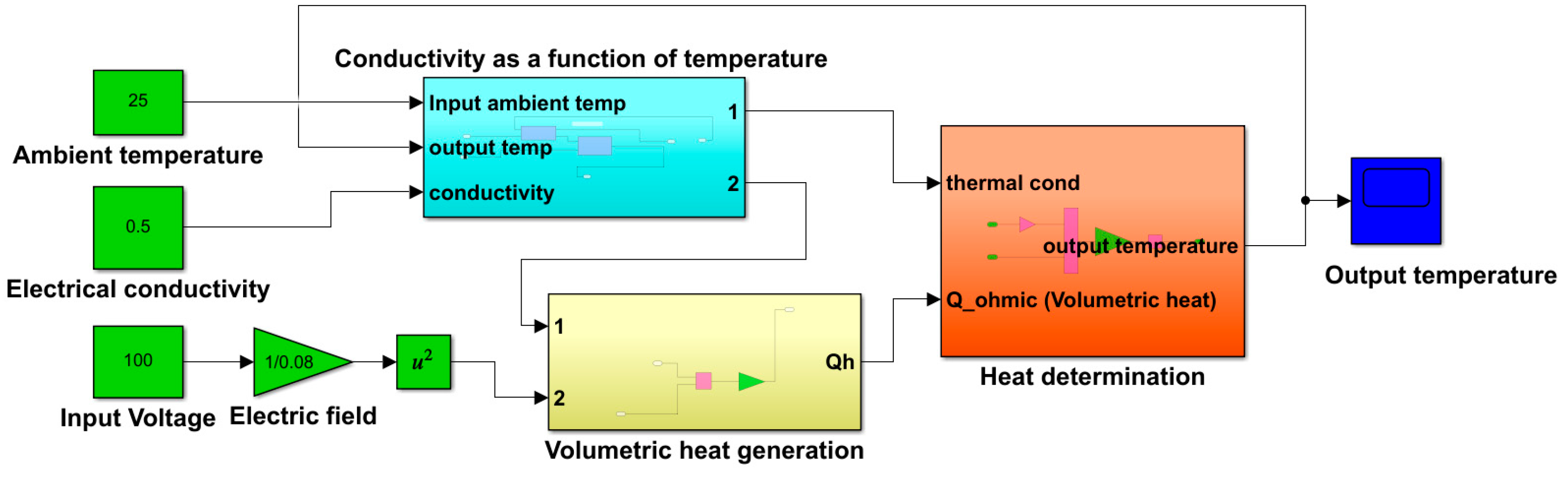
3.3.2. Mathematical Modelling
The mathematical model was developed using SIMULINK, and the governing equations were defined using Simulink blocks. The model defines the Ohmic heater geometry, specifies the thermophysical properties of the food substance, calculates the electrical conductivity as a function of temperature, calculates the volumetric heat within the food as a function of the electric field, and evaluates the final temperature. The Simulink structure and the corresponding subsystems are presented in
Figure 5,
Figure 6 and
Figure 7.
The resulting term gives the rate of change of the food temperature, which can be represented by = ∇·(k·∇T) + . The output temperature is the integral of the signal .
3.3.3. System Identification Technique Overview
The MATLAB system identification toolbox was used to determine a nonlinear model of the Ohmic heating system. Three system identification models were developed:
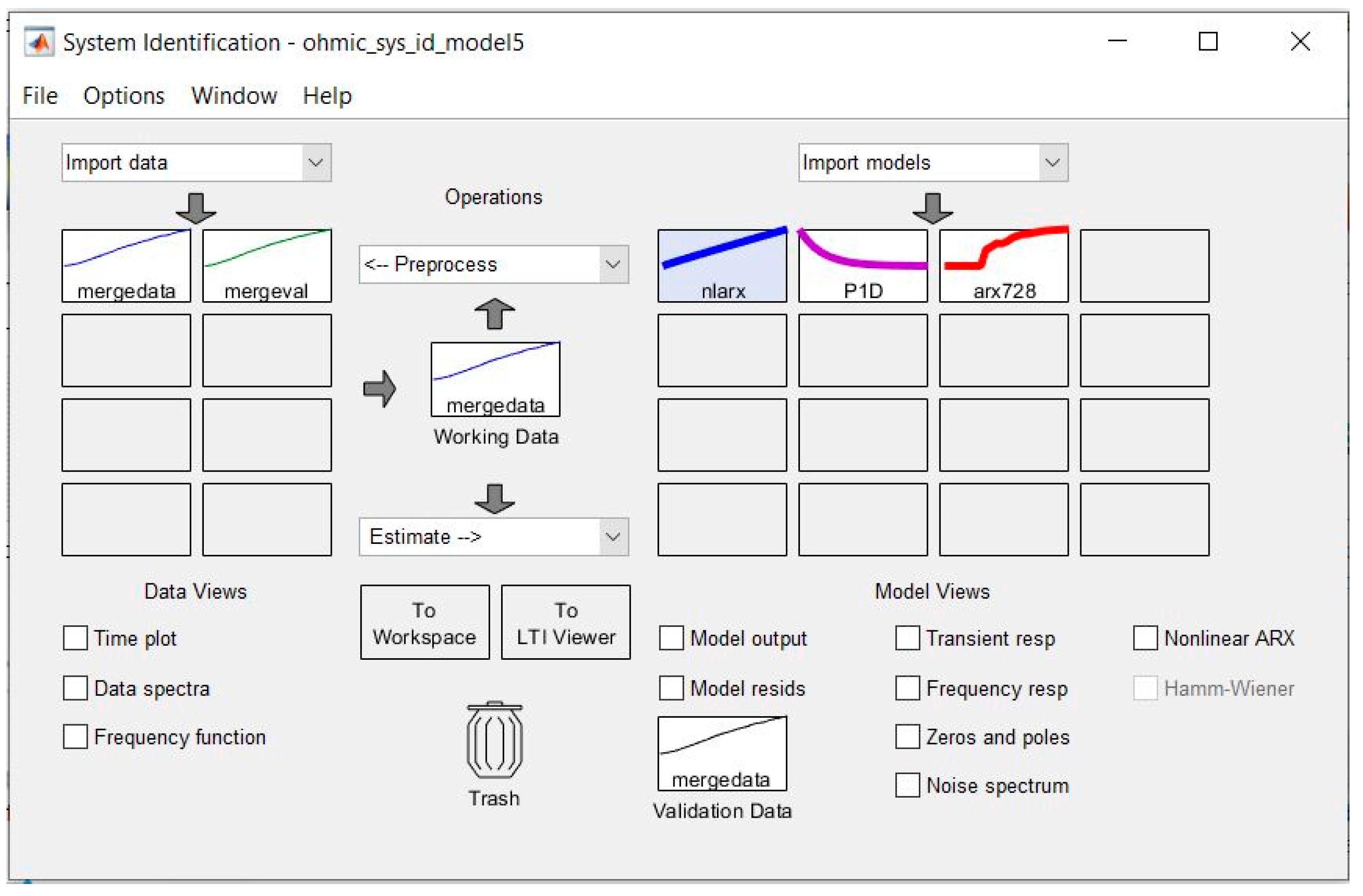
The system identification toolbox of MATLAB was used to develop the models listed above based on the input–output experimental data. This approach does not require mathematical formulae of process dynamics from the user. It is based on empirical data only, and the user is not required to have a complete understanding of the process dynamics. A snapshot of the system identification toolbox interface is shown in
Figure 8 below
- A.
Nonlinear ARX model (nlarx)
The nonlinear ARX model consists of model regressors and a nonlinearity estimator. The nonlinearity estimator comprises both linear and nonlinear functions that act on the model regressors to give the model output.
Given a single input (voltage)/single output (temperature) system, the maximum delay in the input is set to 2 samples, the maximum delay in output is set to 2 samples, and the wavenet is set to 1 unit. Therefore, this model has a total of 4 states given as:
The process model (P1D) is a simple continuous time model that is described in terms of the main time constants, the static gain, a possible dead-time, and a possible process zero (non-constant numerator).
A typical such model is a 1st order transfer function
where K = 4.1975, Tp1 = 805.14, and Td = 0
- C.
Discrete ARX model (arx728)
The ARX model is a linear difference equation that relates the input u(t) to the output y(t) (where t represents the time step), as follows:
The structure is thus entirely defined by the three integers na, nb, and nk. na is the number of poles, nb + 1 is the number of zeros, and nk is the pure time delay (the dead time) in the system. The parameters used here were na = 7, nb = 2, and nk = 8, and the number of free coefficients was set to 9.
3.3.4. System Identification Model Results
The performance of the developed system identification models was based on the best fit estimation and the performance of the residual analysis. Best fit estimation describes the closeness of a predicted output to experimental data. Residual analysis determines the error between a model’s predicted output and validation data from an experiment. If the autocorrelation function falls between the two straight lines, this indicates a very good model.
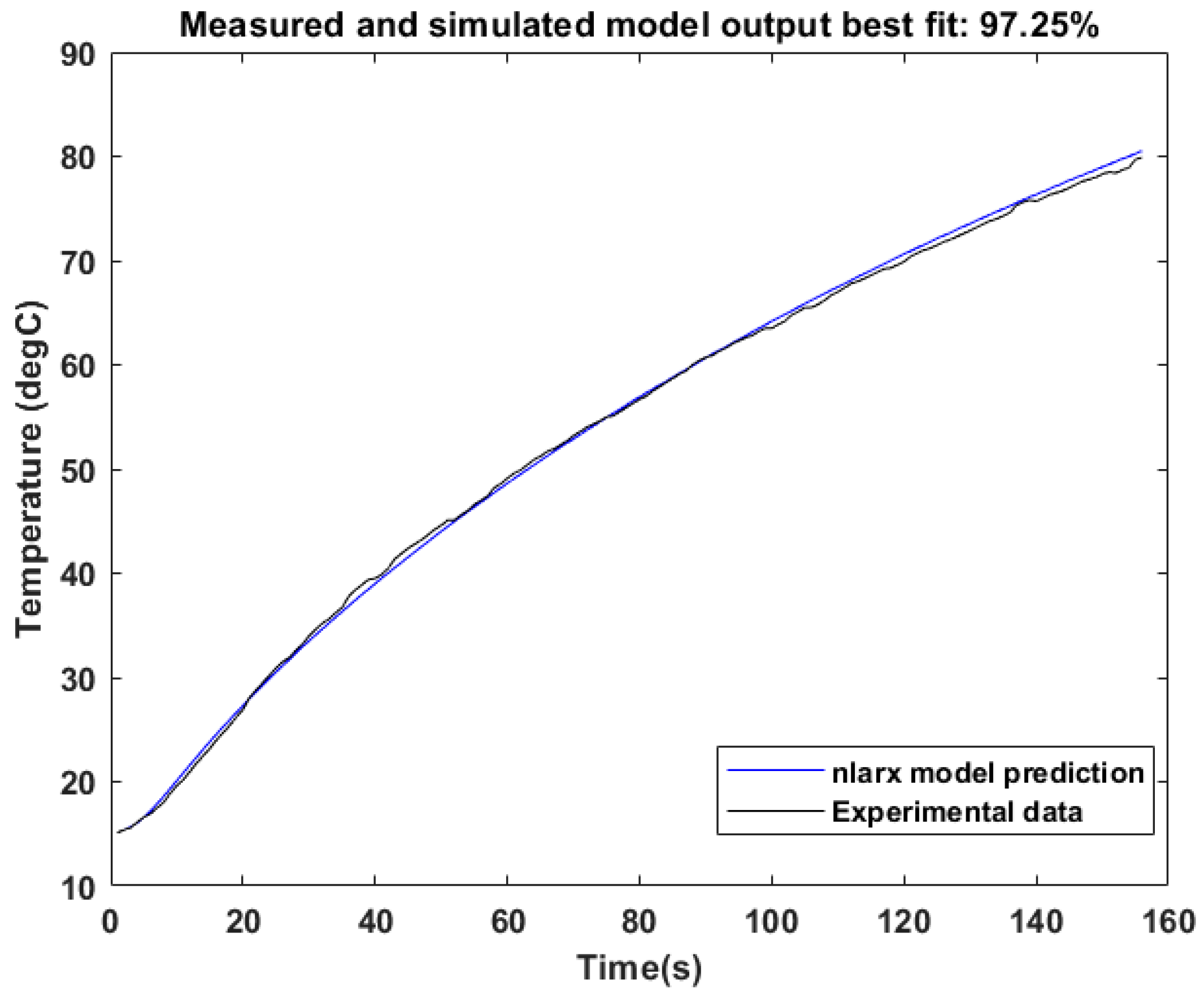
Figure 9 shows that the percent best fit of the simulated output to the measured validation data was 97.25 when heating from 17 °C to a set point of 80 °C. This shows that the model predicted the MEF process with a very high accuracy. Additionally,
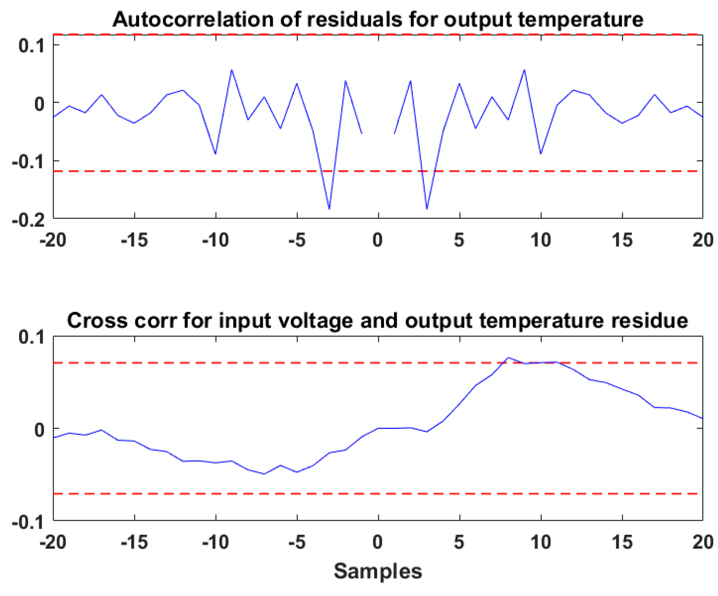
Figure 10 shows that the residual lay mostly within a very confident region (from 0.12 to −0.12), with a tolerance of +−2%, and the cross-correlation function lay between −0.9 and 0.9. Hence, this model was able to represent the MEF process at a high level of confidence.
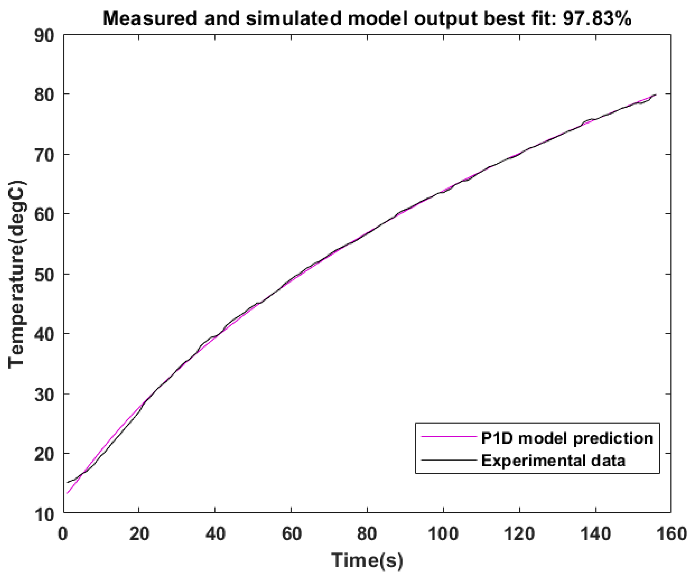
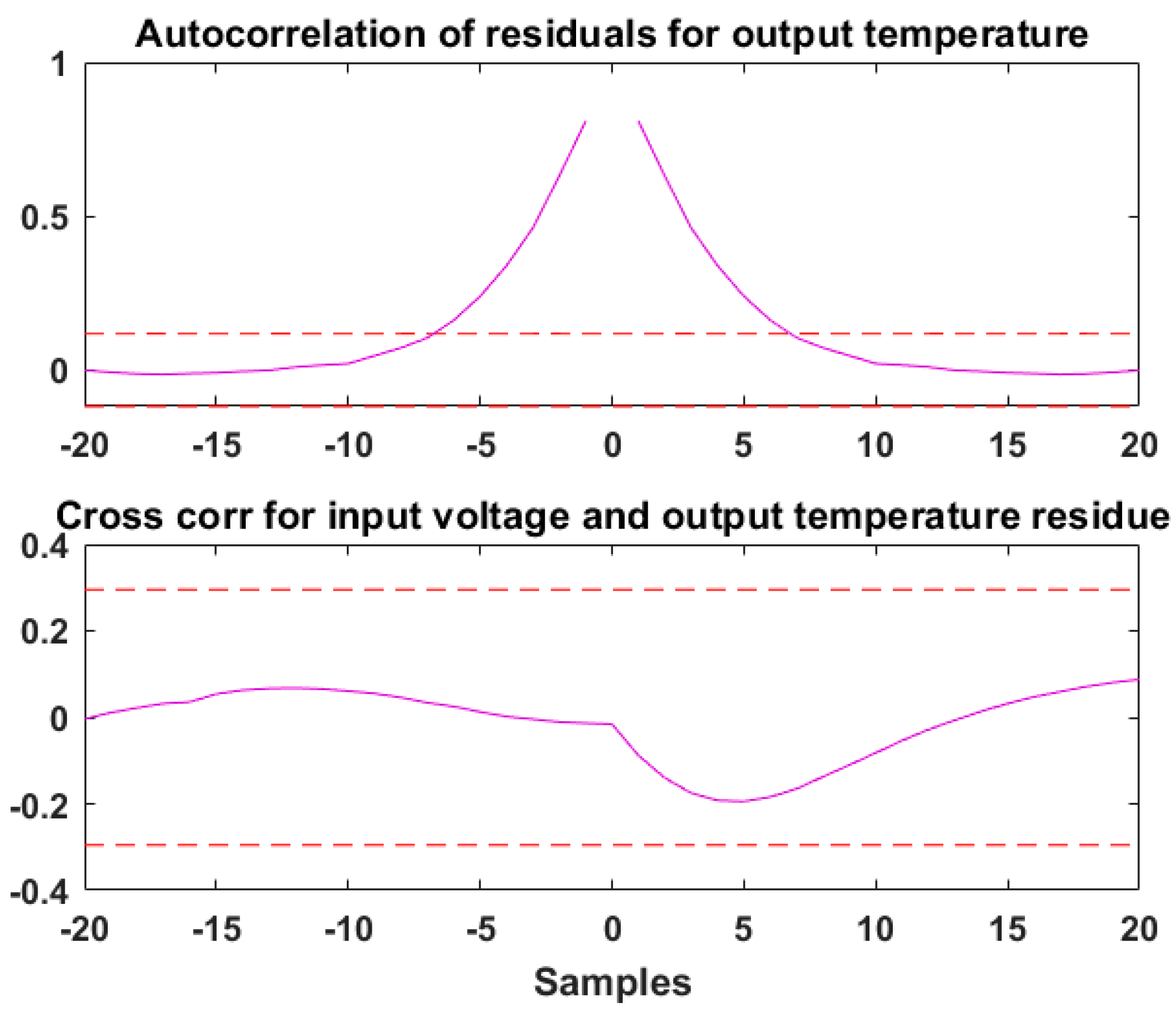
Figure 11 shows that the percent best fit of the simulated output to the validation data was 97.83 when heating from 17 °C to a set point of 80 °C. This shows that the model predicted the MEF process with a very high accuracy.
Figure 12 shows that the residual lay outside the confident region (from 0.12 to −0.12), and the cross-correlation function lay between −1.9 and 0.9. This indicates that the residuals were not correlated and the confidence of the model’s capability of validating actual data was low.
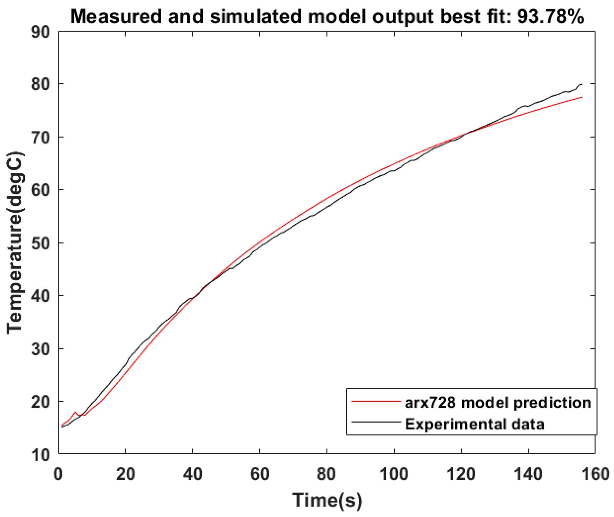
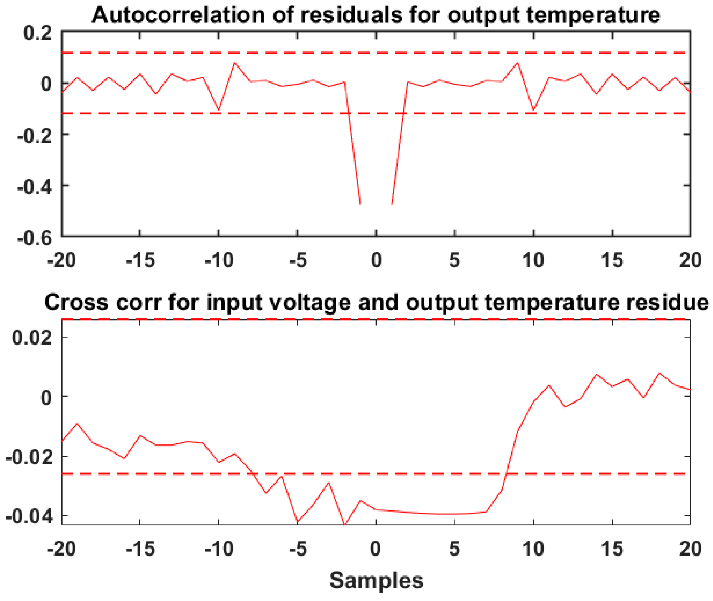
Figure 13 shows that the percent best fit of the simulated output to the validation data of the arx728 model was 93.78 when heating from 17 °C to a set point of 80 °C. This shows that the model predicted the MEF process with a very high accuracy. The residual of the arx728 model lay outside the confidence region (from 0.12 to −0.12), and the cross-correlation function lay outside the range from −0.9 and 0.9, as shown in
Figure 14. This indicates the residuals were not correlated and the confidence of the model’s capability of validating actual data was low.
Based on the performance criteria of the percent best fit plot and the confidence given by the residual and correlation analysis, the nonlinear ARX (nlarx) model was adopted due to its high performance. The autocorrelation plot of the nlarx model stayed within the confidence region during validation.
3.4. Experiment
3.4.1. Food Sample Preparation
The food product used was ‘British fresh whole milk’ purchased at a local supermarket. The initial temperature of the refrigerated milk was between 15 and 17 °C. The initial electrical conductivity of the milk at start-up and initial product temperature was measured using a PC60 Aprea conductivity meter. The volume of milk used for each experiment batch was 500 mL.
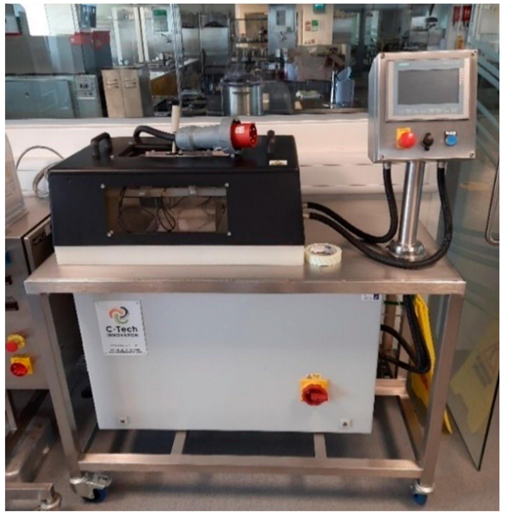
3.4.2. Batch Ohmic Heater
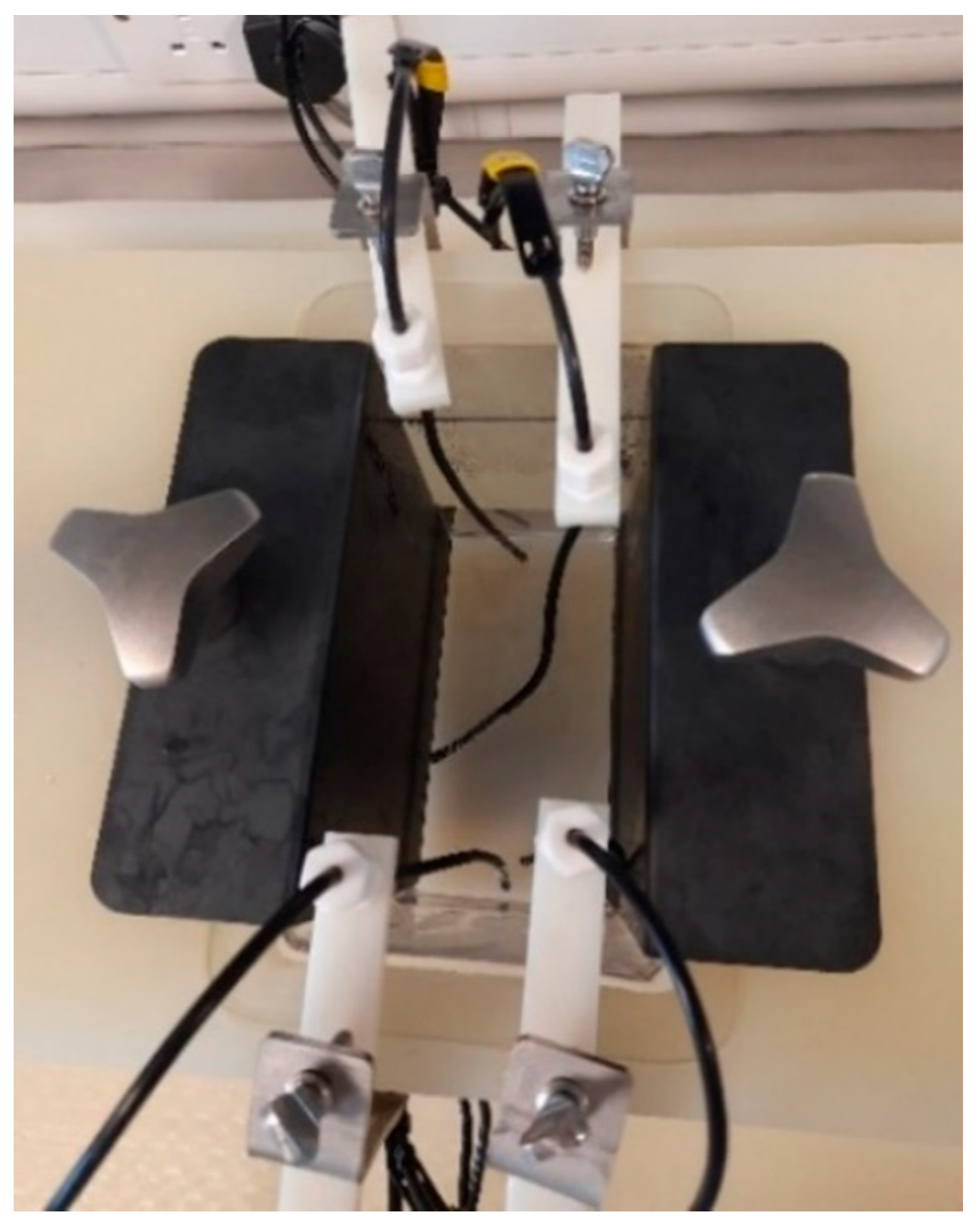
The system was fitted with a control panel and a heating cell with removable titanium (Ti) electrodes. Four thermocouples with variable positions were used to read the temperature. An emergency stop, start/stop/reset switch, and data port for removable flash drives were on the control panel. The set-up and operation of the unit were accessible via the touch screen. The Ti electrode was made of trapezium with a total size 17 × 14.5 × 15.3 × 15 × 0.1 cm (length × length × slant height × height × thickness).
Figure 16 shows the arrangement of the Ti electrodes in the heating cell.
The total size of the heating cell was 17 × 15 × 8 × 9 cm (length × height × width × width). Therefore, the gap between the electrodes was 8 cm at the shortest point and 9 cm at the longest point. During the experiment, given the fixed volume of 500 mL (which corresponded to a height of 4 cm in the heating cell), the shortest gap between the electrodes was 8 cm and the largest gap due to the slant profile was 8.3 cm. The control panel of the Ohmic heater consisted of a voltmeter, an ammeter, a timer, a main switch, and functions for manual/automatic operation. The AC power supply was a 3-phase supply at 50 Hz and 415 V.
4. Model Validation and Results
Experiments using the batch Ohmic heater follow the plan described in
Table 1. For every batch of product heated, the actions in
Table 1 were followed.
To validate the models, temperature data collected from the experiment were compared to the simulated model results. The voltage inputs were also the real-life data measured from the C-Tech Innovation batch Ohmic heater. In the model comparison figures, ‘Ohmic ’ represents the Ohmic heater temperature from experimental data and ‘comsol’, ‘sysid’, and ‘simulink’ represent the COMSOL model, the system identification model, and the Simulink model, respectively. The applied voltage was controlled by a simple PID controller in the C-Tech Innovation batch Ohmic heater. In the following comparison table, ‘Ohmic heater’ represents the experimental data and heating time that were validated against the developed models.
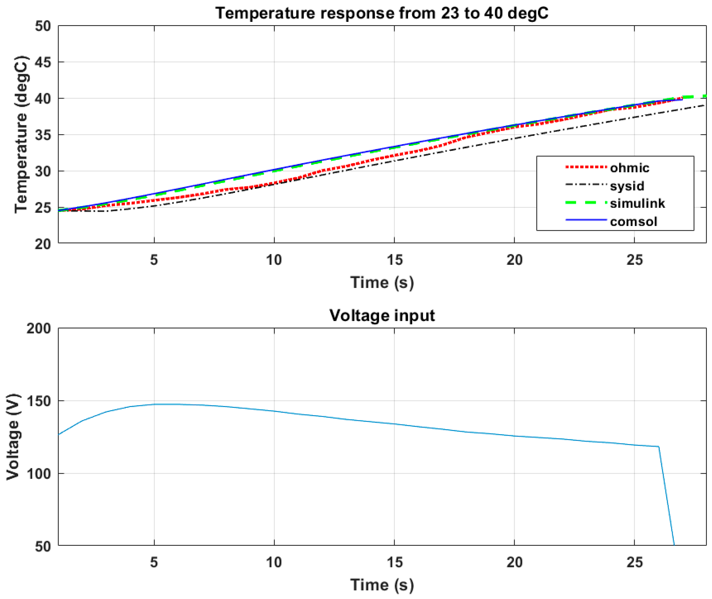
4.1. Validating from 23 to 40 °C
The results presented below show the developed model being validated with experimental data and voltage input. The set point was 40 °C from an initial temperature of 23 °C.
Table 2 shows the steady state error from the set point within a total time of 26 s.
Figure 17 shows that the peak voltage was close to 150 V. This agreed with the equation describing the electrical conductivity as a function of temperature in Equation (3) and the volumetric heat produced in Equation (2). The electrical conductivity was modelled as a function of temperature, so at a lower temperature higher, an electric field was required to produce proportional volumetric heat.
Table 2 shows the prediction performance of the different models in representing the MEF process, which was determined using the set point error as a benchmark. The COMSOL model prediction performance was 98%, the SIMULINK model prediction performance was 99%, and the system identification model prediction performance was 90%.
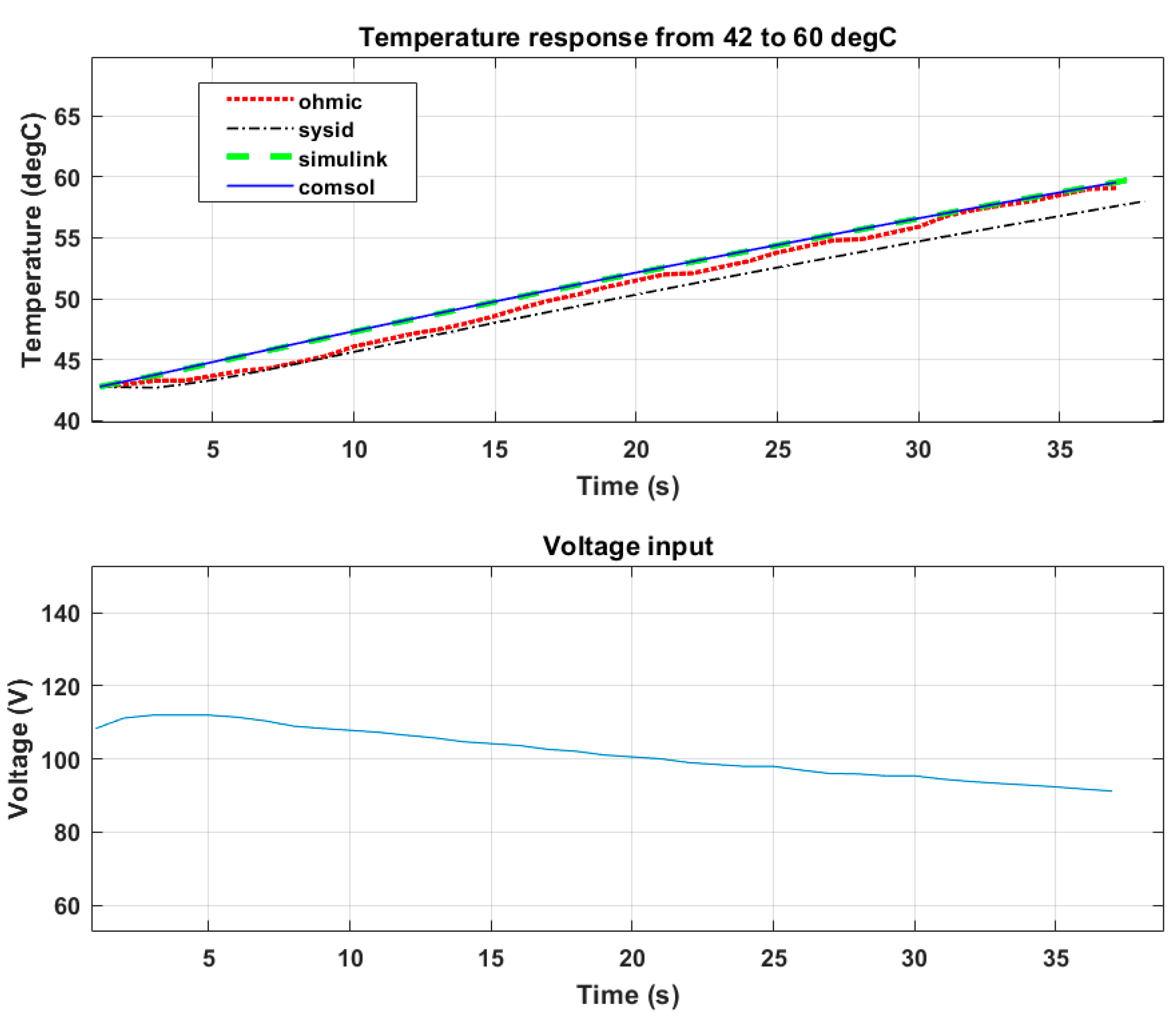
4.2. Validating from 42 to 60 °C
The results presented below show the developed model being validated with experimental data and voltage input. The set point was 60 °C from an initial temperature of 42 °C.
Table 3 shows the steady state error from the set point within a total time of 37 s.
Figure 18 shows that the peak voltage was about 125 V. This shows that with the increased food temperature, a proportional increase in the food conductance was achieved. Therefore, the magnitude of the electric field to raise the food temperature was reduced compared to the results presented
Figure 17. The heating time shown in
Figure 18 was longer than that in
Figure 17 because of the reduced electric field.
Table 3 shows an increase in the set point error in comparison to
Table 2. The increase in set point error could be attributed to an increase in the temperature range of validation. The prediction performance of the COMSOL and SIMULINK models was 97%, while the prediction performance of the system identification model was 86%.
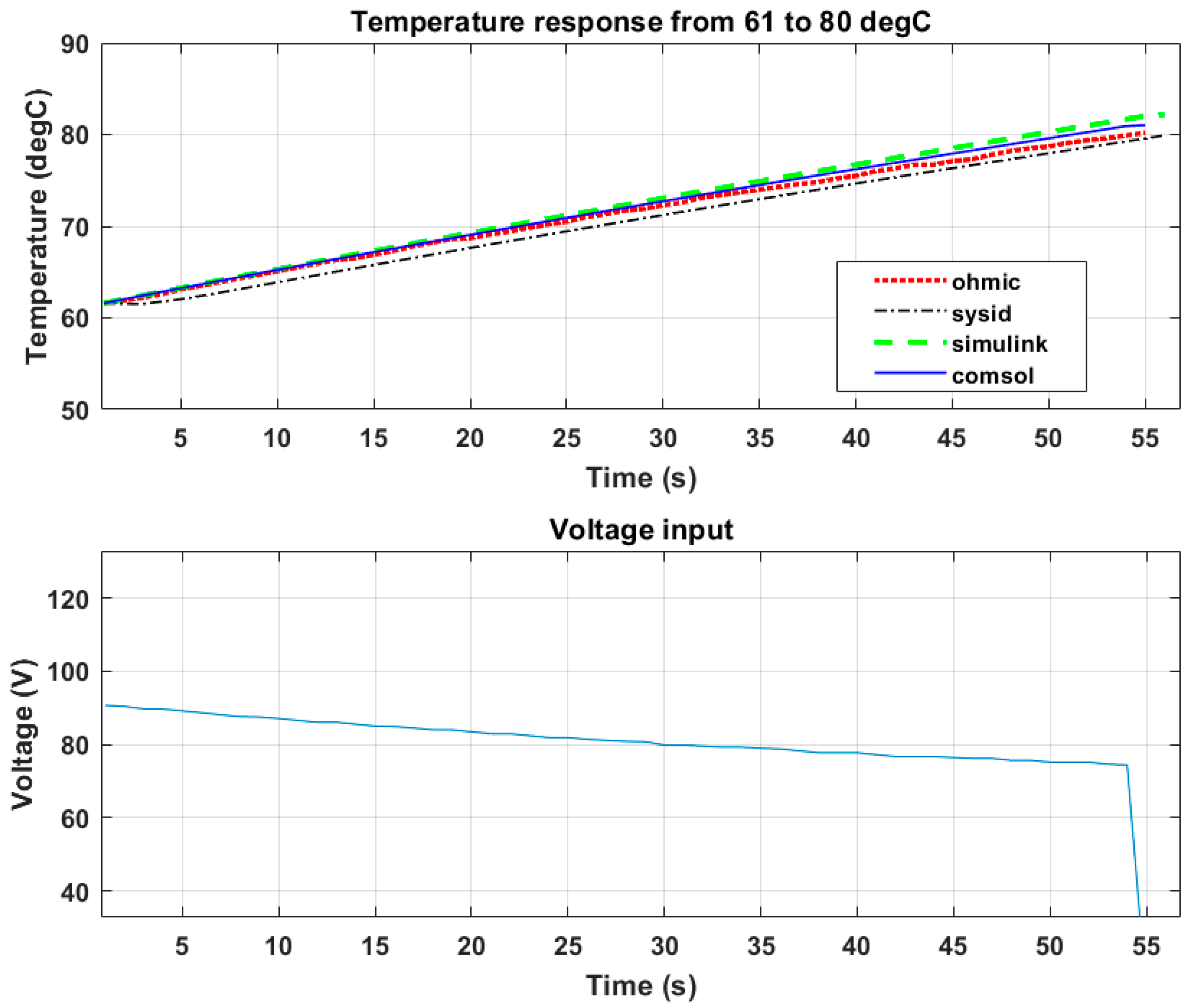
4.3. Validating from 61 to 80 °C
The results presented below show the developed model being validated with experimental data and voltage input. The set point was 80 °C from an initial temperature of 61 °C.
Table 4 shows the steady state error from the set point within a total time of 55 s
Figure 19 shows that the peak voltage from the Ohmic heater was 87 V. The heating time seen in
Figure 19 was longer than that of
Figure 17 and
Figure 18. This shows that the heating time was proportional to the magnitude of the electric field.
Table 4 shows that the COMSOL model had a prediction performance of 94%, the SIMULINK model had a prediction performance of 89%, and the system identification model had a prediction performance of 97%.
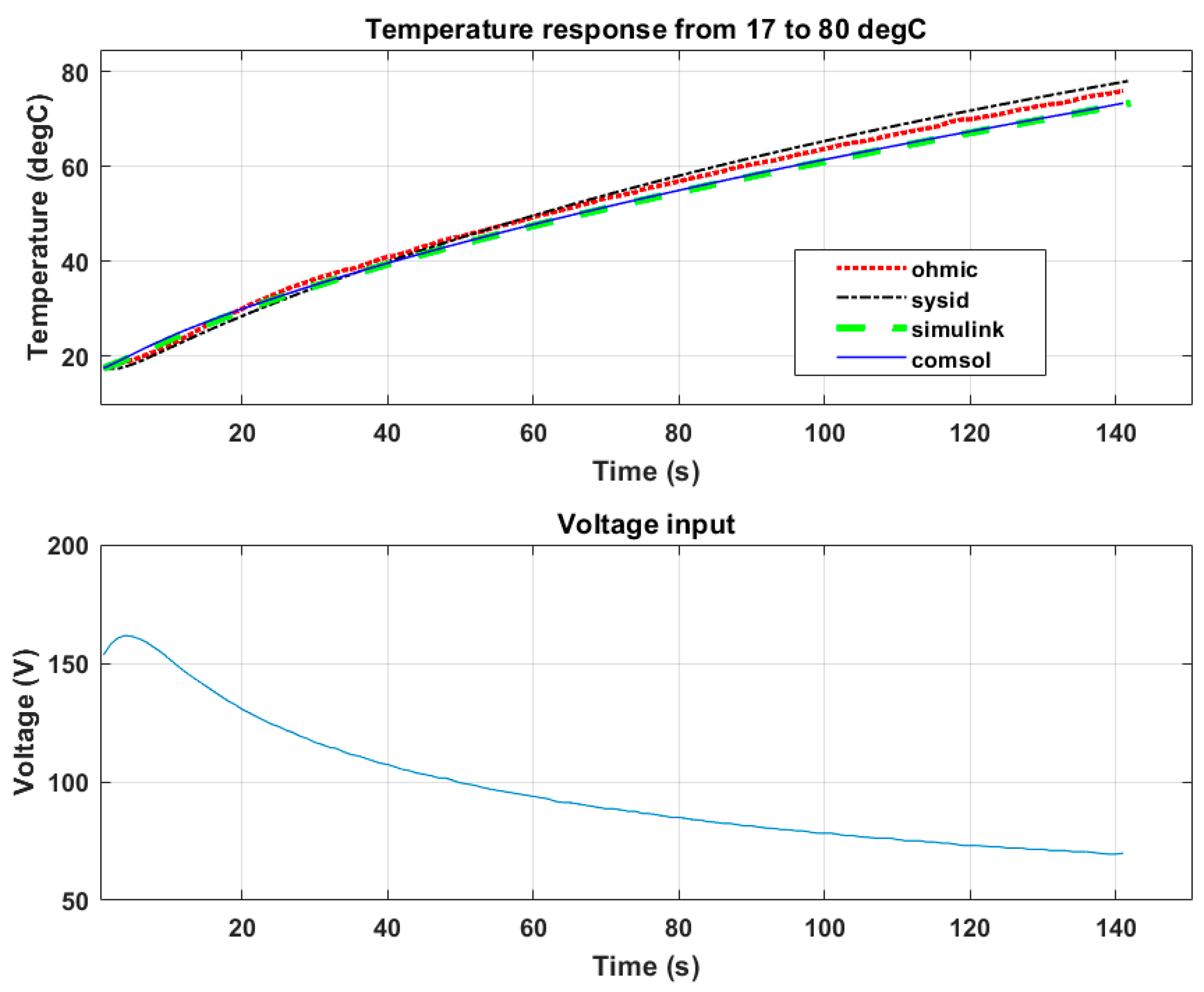
4.4. Validating from 17 to 80 °C
The results presented below show the developed model being validated with experimental data and voltage input. The set point was 80 °C from an initial temperature of 17 °C.
Table 5 shows the steady state error from the set point within a total time of 141 s.
Figure 20 shows that due to the low electrical conductivity at 17 °C, very high electric field was needed to volumetrically raise the temperature of the food. After about 60 s of heating to prevent uncontrolled temperature, the in-built PID controller in the batch Ohmic heater regulated the applied voltage with regard to the set point temperature.
Table 5 shows an increase in the set point error value for a large temperature set point value for both the COMSOL and SIMULINK models. The COMSOL model had a prediction performance of 89%, the SIMULINK block model had a prediction performance of 88%, and the system identification model had a prediction performance of 96%.
5. Conclusions
The authors of this work have presented a novel approach for the modelling and validation of the MEF and OH processes using a range of techniques. Comparisons between a numerical model, a mathematical analytic method, and system identification model were made. The SIMULINK block model illustrated a simpler and ‘close to the real thing’ representation for software requiring lower computational power. The analytical solution obtained from the SIMULINK block model offered a clear view into how the food process variables interacted and affected the result.
The error seen from these models could also be attributed to the errors from the real life PID-produced voltage profile. Given that the PID controller of the batch Ohmic heater was tuned according to the user, errors were transferred to the models being validated by the voltage inputs. These models showed robustness and tolerable error values given that they were validated by a simple PID voltage input from a real-life machine.
The numerical model using COMSOL shows that any OH operation using MEF could be designed and validated using an iterative solution based on the BDF algorithm. The system identification model is a data-driven model based on experimental data. The system identification technique is useful when modelling a highly complex system that cannot be easily represented mathematically. However, the system identification technique can also add intrinsic system experimental errors into the model, so the experimental data must be accurate and post-processed to remove noise.
Future work will model a continuous MEF system that accounts for flow dynamics, including the viscosity and laminar flows of different foods, and relationships with temperature change.


