Theory for Electrochemical Heat Sources and Exothermic Explosions: The Akbari–Ganji Method

Abstract

A device that transforms chemical energy into electrical energy is an electrochemical cell. The reaction type inside the cell determines whether it is exothermic or endothermic. This paper discusses the mathematical modelling of exothermic explosions in a slab. This model is based on a nonlinear equation containing a nonlinear term related to Arrhenius, bimolecular, and sensitised laws of reaction kinetics. The absolute temperature can be derived by solving the nonlinear equation using the Akbari–Ganji technique. The mathematical model also numerically solved and simulated in the MATLAB^® v2016b software. The new simple theoretical result is validated with previously identified analytical and numerical findings. The influence of the parameters of Frank-Kamenetskii number, activation energy and the numerical exponent on temperature is discussed. The Frank-Kamenetskii number is observed to drop as the temperature is found to decrease, while the activation energy parameter is shown to increase. The numerical exponent has little or no effect on the temperature. An extension of this model to cylinder and sphere geometry is also provided.

1. Introduction

Numerous industries, such as heavy oil recovery, the storage of cellulosic compounds, coal gasification, waste burning, biomass and coal combustion, and lithium-ion batteries, have researched the thermal breakdown of reactive materials due to exothermic chemical reactions. Thus, it is highly desirable to model the situation mathematically. Many researchers have provided models to explain abusive behaviour and thermal runaway. Hatchard et al. [1] took the initial steps to explain the exothermic reaction kinetics in prismatic and cylindrical lithium-ion cells. Furthermore, they accurately predicted the variation in cell temperature during and after nail penetration using a numerical simulation. A modified reaction–diffusion theory was provided in the works of Kim et al. [2] and Peng et al. [3,4]. An electrochemical model of lithium-ion battery nail penetration, which involved a dramatic temperature change, was also discussed in [5]. A catastrophe theory approach based on a simplified ordinary differential equation has also been reported [6]. This model was extended in [7,8].

Ziebert et al. [9] discussed electrochemical–thermal characterization and thermal modelling for batteries. Guo et al. [10] developed the three-dimensional thermal finite element modelling of lithium-ion batteries in thermal abuse applications. In 1930, Semonov, Zeldovith, and Frank-Kamenetskii described this behaviour first, and their pioneering contributions were presented in [11]. Frank-Kamenetskii also proposed the steady-state theory of thermal explosions. This idea has been applied to various combustible material geometries in the literature. For an infinite slab, Boddington et al. [12,13,14] and Wake et al. [15] reviewed a case of two-step parallel exothermic processes, and they extended the investigations to two other geometries of an infinite circular cylinder and a sphere. Balakrishnan et al. [16] obtained critical values for some geometries, such as infinite squares, rods, and cubes, using the finite difference method.

Makinde et al. [17] obtained analytical solutions for the governing nonlinear boundary value problem using the perturbation technique and Hermite–Pade approximants. Also, they discussed the essential properties of a temperature field, including bifurcations and thermal criticality. Ananthasamy et al. [18] used the homotopy analysis method to solve a nonlinear equation to obtain an analytical expression of the temperature in an exothermic explosion in a slab. This is time-consuming since it contains an infinite number of convergence control parameters. Er-Riani and Chetehouna [19] applied the homotopy perturbation method to solve the steady-state nonlinear equation in an exothermic chemical reaction. This perturbation method has a convergence problem, however, and requires a small parameter. In this paper, we obtain a simple analytical expression for the temperature field for a range of kinetic mechanisms, such as sensitised, Arrhenius, and bimolecular reactions, by solving the nonlinear Frank-Kamenetskii equation using the very useful Akbari–Ganji method.

2. Mathematical Formulation and Analysis of the Problems

Considering the steady state of an exothermic chemical reaction in a combustible slab with the potential of heat loss to the environment, Frank-Kamenetskii [11] first proposed the classical formulation of this problem. The heat balance equation for steady-state conditions is given as follows [19]:

$$k \frac{d^{2}T\left(Y\right)}{d Y^2}+Q C_0 A {\left(\frac{K T\left(Y\right)}{v h}\right)}^m{e}^{\frac{-E}{R T\left(Y\right)}}=0$$

(1)

The boundary conditions are

$$\frac{d T}{d Y}=0 \mathrm{at} Y=0,$$

(2)

$$T=T_0 \mathrm{at} Y=a,$$

(3)

where $T$ denotes the absolute temperature, $k$ represents the material’s thermal conductivity, $Q$ is the heat of the reaction, $C_0 \mathrm{i}\mathrm{s}$ the initial concentration of the reactant species, $A \mathrm{i}\mathrm{s}$ the rate constant, $h$ indicates Planck’s number, $v$ denotes the vibration frequency, $K$ is Boltzmann’s constant, $E$ represents the activation energy, $R$ is the universal gas constant, $a$ is the slab half width, $Y$ is the distance measured in the normal direction in the plate, and $T_0$ is the wall temperature. The parameter m is the numerical constant, so that m = 2, 0, 1/2 indicates the numerical exponent for sensitised, Arrhenius, and bimolecular kinetics. To reduce the complexity, we make the nonlinear Equation (1) into a dimensionless form by defining the following dimensionless parameters:

$$\theta =\frac{E (T-T_0)}{R T_0^2}, \epsilon =\frac{R{T}_0 }{E}, y=\frac{Y}{a}, \lambda =\frac{Q E A a^2{C}_0 K^m{T}_0^{m-2}{e}^{\frac{E}{R{T}_0}}}{v^m h^{m}R k}$$

(4)

where $\theta$ is the dimensionless temperature field, $\lambda$ denotes the Frank-Kamenetskii parameter, $\epsilon$ represents the activation energy parameter, and $y$ is the dimensionless distance. If the Frank-Kamenetskii parameter λ is greater than a critical value, an explosion occurs and the differential equation does not have a solution. Using Equation (4), Equation (1) reduces this to the following dimensionless form:

$$\frac{d^2\theta \left(y\right)}{d y^2}+\lambda {(1+\epsilon \theta \left(y\right))}^m{e}^{\left(\frac{\theta \left(y\right)}{1+\epsilon \theta \left(y\right)}\right)}=0$$

(5)

The dimensionless boundary conditions are

$$\frac{d \theta }{d y}=0 \mathrm{at} y=0,$$

(6)

$$\theta =0 \mathrm{at} y=1,$$

(7)

3. New Analytical Expression of the Temperature Distribution Using the Akbari–Ganji Method

The Taylor series [20,21], Adomian decomposition [22], variational iteration [23], and Akbari–Ganji methods [24] are only a few of the asymptotic techniques that have been applied to solve nonlinear differential equations. Among these techniques, the AGM (discussed in Appendix A) might be regarded as a useful algebraic (semi-analytic) approach to resolving such issues. According to the AGM, a solution function with unidentified constant coefficients is supposed to satisfy the differential equation and the initial conditions. We can assume that the trial solution of Equation (5) is

$$\theta \left(y\right)={{\sum }_{i=0}^2{\theta }_i y^i=\theta }_0+{\theta }_{1}y+{\theta }_2{y}^2$$

(8)

where ${\theta }_0, {\theta }_1, \mathrm{a}\mathrm{n}\mathrm{d} {\theta }_2$ are constants. Using the boundary conditions (6) and (7), we obtain

$${\theta }_1=0, {\theta }_0=-{\theta }_2$$

(9)

Now, we can define the function $G$ by

$$G\left(y\right)=\frac{d^2\theta }{d y^2}+\lambda {(1+\epsilon \theta )}^m{e}^{\left(\frac{\theta }{1+\epsilon \theta }\right)}=0$$

(10)

Using Equation (8), Equation (10) at $y=0$ becomes

$$G\left(y=0\right)={2 \theta }_2+\lambda {(1-\epsilon {\theta }_2)}^m{e}^{\left(\frac{{-\theta }_2}{1-\epsilon {\theta }_2}\right)}=0$$

(11)

Using Equation (9), Equation (8) can be rewritten as follows:

$$\theta \left(y\right)={\theta }_2\left(y^2-1\right)$$

(12)

The parameter ${\theta }_2$ is obtained by solving the nonlinear Equation (13).

$${2 \theta }_2+\lambda {(1-\epsilon {\theta }_2)}^m{e}^{\left(\frac{{-\theta }_2}{1-\epsilon {\theta }_2}\right)}=0$$

(13)

The unknown parameter ${ \theta }_2$ can be obtained by solving Equation (13) using Matlab R2019b or Wolfram Alpha.com (free online software, accessed on 4 September 2023).

4. Previous Analytical Results

The homotopy analysis method and the perturbation methodology may both be utilised to solve the nonlinear Equation (5) efficiently, as suggested by Anathaswamy’s work [18] and Makinde et al.’s study [17]. The lengthy expressions obtained in the aforementioned publications may cause some convergence issues for inexperienced users. Therefore, we tackle the problem directly in our paper using the AGM method which has been found effective for analysing transport and kinetics in bounded regions [24,25]. This methodology provided approximate closed form expressions for the temperature distribution in the region, which is in good agreement with numerical simulations.

5. Discussion

Equation (12) represents the simplest analytical expression of the temperature profile. The thermal decomposition of the reacting combustible material depends on the parameters $\lambda$, $\epsilon \mathrm{a}\mathrm{n}\mathrm{d} m$, which are of great importance to applications in industrial safety and the handling techniques of explosives.

Numerical Simulation

This section validates the above theoretical results using a numerical simulation for physically realistic values of various embedded parameters. The function bvp4c in Matlab/Scilab software (Version 9.11), which solves nonlinear boundary value problems for ordinary differential equations, is used to solve these equations numerically. The present (AGM) and previous (HAM, PM) analytical results are compared to this numerical solution in

Table 1. Comparison of dimensionless temperature field $\theta \left(y\right)$ with simulation results and previous analytical results for $\lambda =0.1$, $\epsilon =0.1, m=-2 \mathrm{a}\mathrm{n}\mathrm{d} {\theta }_2=-0.05175$.

$\mathit{y}$	$\mathit{\theta }\left(\mathit{y}\right)$
	Num.	AGM Equation (12) This Work	HAM [18]	PM [17]	Error % AGM Equation (12) This Work	Error % HAM [18]	Error % PM [17]
0	0.0517	0.0517	0.0517	0.0516	0.0000	0.0000	0.1934
0.2	0.0496	0.0496	0.0496	0.0495	0.0000	0.0000	0.2016
0.4	0.0432	0.0436	0.0434	0.0433	0.9259	0.0230	0.4629
0.6	0.0327	0.0324	0.0330	0.0329	0.9174	0.0303	0.6116
0.8	0.0179	0.0180	0.0185	0.0185	0.5586	3.3519	3.3519
1	0.0000	0.0000	0.0000	0.0000	0.0000	0.0000	0.0000
	Average error (%)				0.3493	0.5675	0.8036

,

Table 2. Comparison of dimensionless temperature field $\theta \left(y\right)$ with simulation results and previous analytical results for $\lambda =0.5$, $\epsilon =0.1, m=-2, { \mathrm{a}\mathrm{n}\mathrm{d} \theta }_2=-0.320092$.

$\mathit{y}$	$\mathit{\theta }\left(\mathit{y}\right)$
	Num.	AGM Equation (12) This Work	HAM [18]	PM [17]	Error % AGM Equation (12) This Work	Error % HAM [18]	Error % PM [17]
0	0.3045	0.3201	0.2951	0.2823	4.8133	3.0870	7.2906
0.2	0.2916	0.3001	0.2829	0.2707	2.8000	2.9835	7.1673
0.4	0.2532	0.2548	0.2466	0.2363	0.6319	2.5671	6.6745
0.6	0.1899	0.1893	0.1869	0.1792	0.3159	1.5798	5.6334
0.8	0.1031	0.1030	0.1041	0.1002	0.0970	0.9699	2.8128
1	0.0000	0.0000	0.0000	0.0000	0.0000	0.0000	0.0000
	Average error (%)				1.4430	1.8645	4.9298

,

Table 3. Comparison of dimensionless temperature field $\theta \left(y\right)$ with simulation results and previous analytical results for $\lambda =0.1$ when $\epsilon =0.1, m=0, { \theta }_2=-0.0523$.

$\mathit{y}$	$\mathit{\theta }\left(\mathit{y}\right)$
	Num.	AGM Equation (12) This Work	HAM [18]	PM [17]	Error % AGM Equation (12) This Work	Error % HAM [18]	Error % PM [17]
0	0.0522	0.0523	0.0521	0.0522	0.1916	0.1916	0.0000
0.2	0.0501	0.0501	0.0500	0.0501	0.0000	0.1996	0.0000
0.4	0.0436	0.0437	0.0437	0.0438	0.2294	0.2294	0.4587
0.6	0.0329	0.0331	0.0332	0.0333	0.6079	0.9118	1.2158
0.8	0.0180	0.0181	0.0188	0.0187	0.5555	4.4444	3.8889
1	0.0000	0.0000	0.0000	0.0000	0.0000	0.0000	0.0000
	Average error (%)				0.2641	0.9961	0.9272

and

Table 4. Comparison of dimensionless temperature field $\theta \left(y\right)$ with simulation results and previous analytical results for $\lambda =0.4$, $\epsilon =0.1, m=0, {\theta }_2=-0.32181$.

$\mathit{y}$	$\mathit{\theta }\left(\mathit{y}\right)$
	Num.	AGM Equation (12) This Work	HAM [18]	PM [17]	Error % AGM Equation (12)	Error % HAM [18]	Error % PM [17]
0	0.3255	0.3208	0.3192	0.3172	1.4439	1.9355	2.5499
0.2	0.3116	0.3077	0.3059	0.3040	1.2516	1.8292	2.4390
0.4	0.2701	0.2684	0.2662	0.2646	0.6294	1.4439	2.0363
0.6	0.2021	0.2030	0.2011	0.1994	0.4433	0.4948	1.3360
0.8	0.1093	0.1113	0.1117	0.1110	1.8230	2.1958	1.5553
1	0.0000	0.0000	0.0000	0.0000	0.0000	0.0000	0.0000
	Average error (%)				0.9319	1.3163	1.6527

. The maximum average relative error between our result and the simulation result is 1.44%. But the maximum error between numerical results and HAM and PM is 1.86% and 4.92%, respectively. In the computations, we solve the Frank-Kamenetskii equation for the kinetic cases where m = −2 and m = 0 corresponding to sensitised and Arrhenius kinetics.

6. Limiting Case

We now examine the general expression presented in Equation (5) and look at the case when the activation energy parameter is small so εθ << 1. Under such circumstances, Equation (5) becomes

$$\frac{d^2\theta }{d y^2}+\lambda e^{\theta }=0$$

(14)

In this case, the temperature profile becomes

$$\theta \left(y\right)=log\left[\frac{n-n{Tanh}^2(0.5y \sqrt{n})}{2\lambda }\right]$$

(15)

where n is obtained from the equation

$$n-n{Tanh}^2\left(0.5\sqrt{n}\right)=2\lambda$$

(16)

In

Table 5. Comparison of our approximate analytical result (12) with the exact result (19) for the limiting case.

$\mathit{y}$	$\mathit{\lambda }=0.1$			$\mathit{\lambda }=0.3$			$\mathit{\lambda }=0.5$
	Exact Solution Equation (15)	AGM Equation (12)	Error %	Exact Solution Equation (15)	AGM Equation (12)	Error %	Exact Solution Equation (15)	AGM Equation (12)	Error %
0	0.0522	0.0527	0.9578	0.1733	0.1795	3.5776	0.3290	0.3474	5.5927
0.2	0.0501	0.0505	0.7984	0.1661	0.1689	1.6857	0.3148	0.3246	3.1131
0.4	0.0436	0.0439	0.6881	0.1443	0.1440	0.2079	0.2728	0.2768	1.4663
0.6	0.0329	0.0330	0.3039	0.1085	0.1087	0.1843	0.2040	0.2060	0.9804
0.8	0.0180	0.0180	0.0000	0.0590	0.0590	0.0000	0.1102	0.1102	0.0000
1	0.0000	0.0000	0.0000	0.0000	0.0000	0.0000	0.0000	0.0000	0.0000
	Average error (%)		0.4580	Average error (%)		0.9426	Average error (%)		1.8587

, we compare the approximate analytical result obtained using the AGM presented in Equation (12), with the analytical solution outlined in Equation (15) for the limiting case when εθ << 1. We can notice that the average error percentage between the AGM and an exact limiting case result (Equation (15)) did not exceed 1.8% for the slab geometry. This is an indication of the usefulness of the AGM.

7. Influence of the Parameters on Temperature

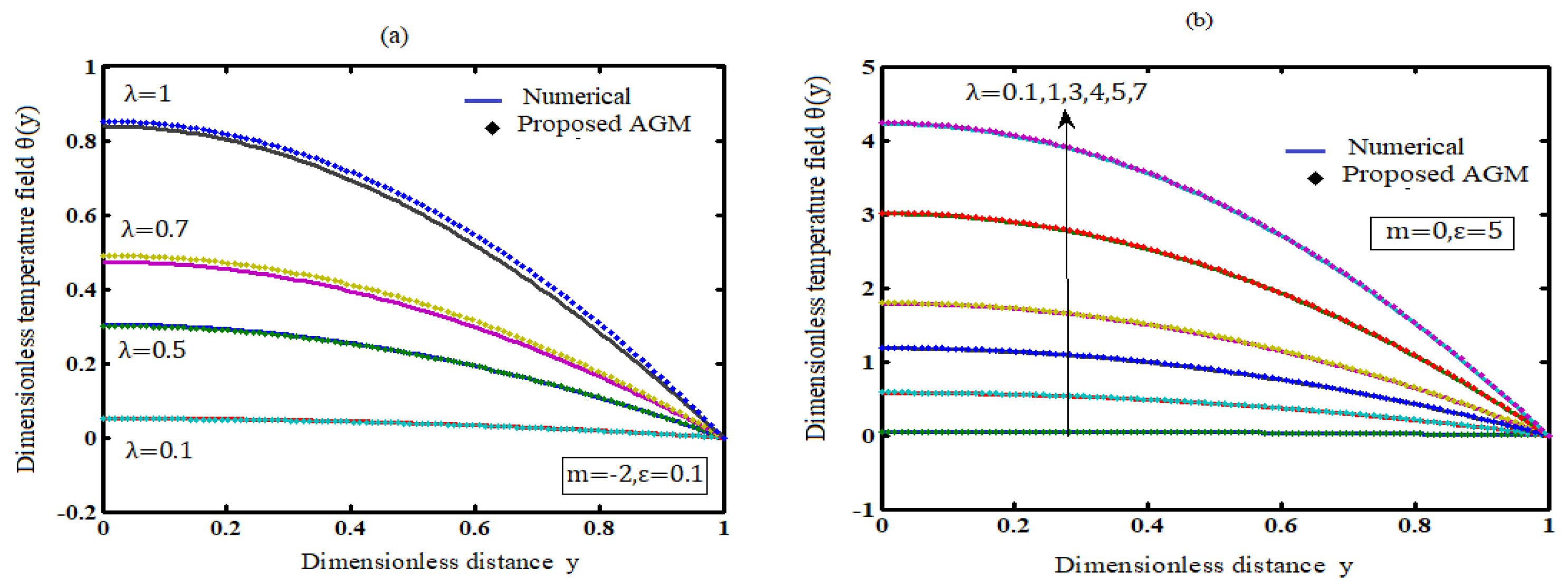
7.1. Influence of the Frank-Kamenetskii Parameter $\lambda$ on Temperature

Figure 1 illustrates the effects of the Frank-Kamenetskii parameter on a temperature profile for the various reaction mechanisms. From the figure, it is observed that the rate of an exothermic reaction increased with the increase in the Frank-Kamenetskii parameter. The slab internal heat generation caused by the exothermic reaction increased as the Frank-Kamenetskii parameter increased. The slab temperature invariably rises as a result of this.

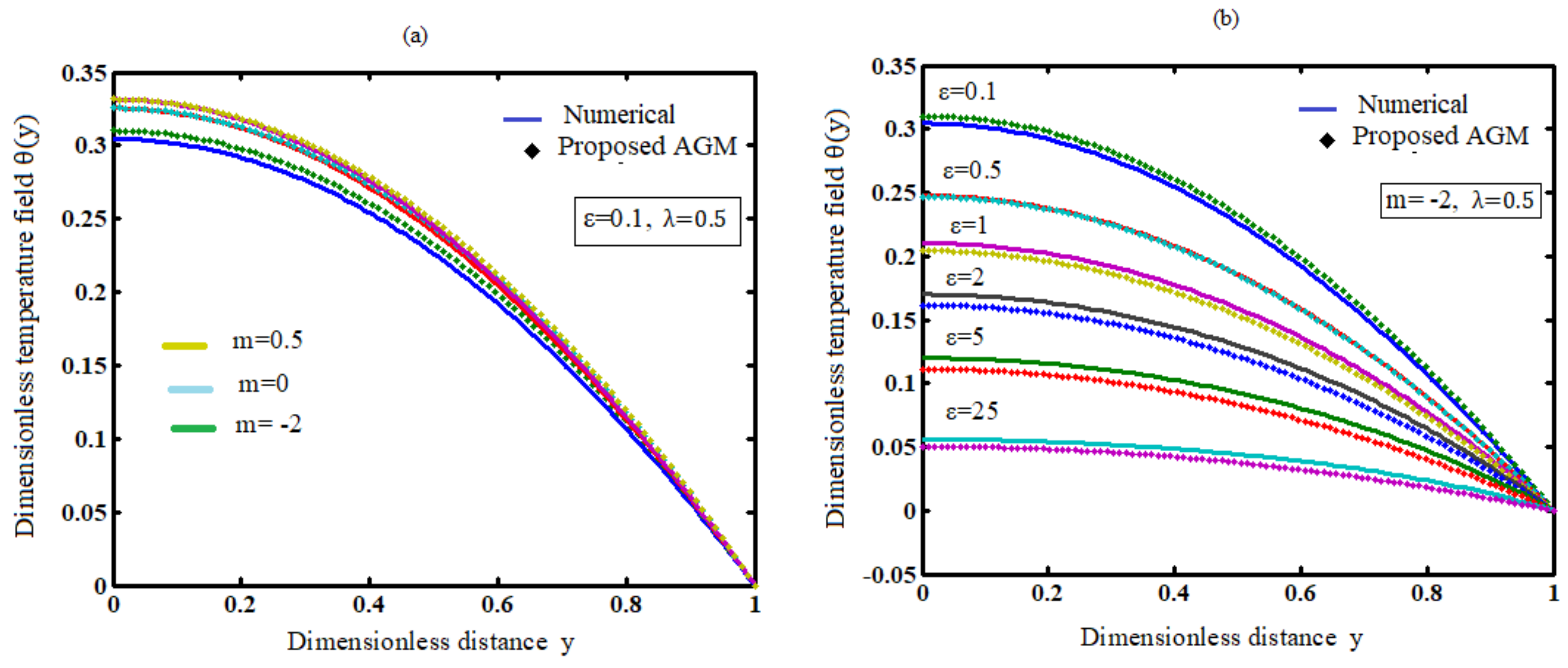
7.2. Influence of the Numerical Exponent (m) on Temperature

The effects of the numerical exponent m, defining the type of reaction kinetics, on the temperature profiles are shown in Figure 2a. The figure shows that the temperature increased as the numerical exponent number m increased. Moreover, the tables and figures show that in the bimolecular (m = 0.5) type of exothermic reaction, a thermal explosion occurred faster than in the Arrhenius (m = 0) and sensitised (m = −2) reactions.

7.3. Influence of the Activation Energy Parameter (ε) on Temperature

A similar effect of temperature was observed with increasing values of the activation energy parameter (ε). The influence of the activation energy parameter on the temperature profile is shown in Figure 2b. With rising values of the activation energy parameter ε, a similar effect of temperature enhancement was observed. Increasing values of ε imply that the reacting slab’s activation energy was insufficient, and thus the reacting slab’s volatility characteristic was significantly reduced.

The overall activation energy of the process reduced as the temperature rose (Figure 2b). Faster Li ion diffusion is directly correlated with lower activation energy, which leads to higher power outputs from the electrode. Thus, our analytical result will help to develop higher-power batteries and electrode materials with faster ionic diffusion in lithium-ion cells.

7.4. Extension of the Theoretical Model for Cylindrical and Spherical Geometries

This section briefly indicates some extensions to the theoretical model outlined in this paper. The nonlinear reaction–diffusion equation for cylindrical and spherical geometries can be written as follows [19]:

$$\frac{d^2\theta }{d y^2}+\frac{j}{y}\frac{d\theta }{d y}+\lambda {(1+\epsilon \theta )}^m{e}^{\left(\frac{\theta }{1+\epsilon \theta }\right)}=0$$

(17)

where j = 0, 1, and 2 represent the geometry factors for the slab, cylinder, and sphere. The dimensionless boundary conditions are

$${\theta }^{\prime }\left(0\right)=0$$

(18)

$$\theta \left(1\right)=0$$

(19)

We can assume that the equation’s solution has the following form:

$$\theta \left(y\right)={{\sum }_{i=0}^2{\theta }_i y^i=\theta }_0+{\theta }_{1}y+{\theta }_2{y}^2$$

(20)

where ${\theta }_0,{\theta }_1, \mathrm{a}\mathrm{n}\mathrm{d} {\theta }_2$ are constants. Using the boundary conditions (18) and (19), we obtain

$${\theta }_1=0, {\theta }_0=-{\theta }_2$$

(21)

Now, Equation (20) becomes

$$\theta \left(y\right)={\theta }_2{y}^2-{\theta }_2$$

(22)

The function $G$ will now be defined by

$$G\left(y\right)=\frac{d^2\theta }{d y^2}+\frac{j}{y}\frac{d\theta }{d y}+\lambda {(1+\epsilon \theta )}^m{e}^{\left(\frac{\theta }{1+\epsilon \theta }\right)}=0$$

(23)

Using Equation (22), Equation (23) at $y=0.5$ becomes

$$G\left(y=0.5\right)={2 \theta }_2(1+j)+\lambda {(1-0.75{\theta }_2 \epsilon )}^m{e}^{\left(\frac{{-0.75 \theta }_2}{1-0.75 {\theta }_{2 \epsilon }}\right)}=0$$

(24)

Hence, the solution of Equation (17) is

$$\theta \left(y,\lambda ,\epsilon , m,j\right)={\theta }_2\left(y^2-1\right)$$

(25)

Here, ${\theta }_2$ is obtained by solving the nonlinear Equation (26).

$${2 \theta }_2(1+j)+\lambda {(1-0.75{\theta }_2 \epsilon )}^m{e}^{\left(\frac{{-0.75 \theta }_2}{1-0.75 {\theta }_{2 \epsilon }}\right)}=0$$

(26)

The above nonlinear equation can be solved using wolframalpha.com for the given values of dimensionless parameters $\lambda , j$ and $\epsilon$.

Figure 3 compares the simulation results for the three geometries with the analytical expression. Based on the figure, the temperature in spherical geometries is assumed to be lower than in slabs.

8. Conclusions

We studied the exothermic explosion of a viscous combustible in slab, cylinder, and spherical geometries under Arrhenius, bimolecular, and sensitised laws of reaction schemes. The steady-state exothermic chemical reaction in a slab of combustible material was considered. We proved that this method provides an excellent approximation of the solution of this nonlinear system with high accuracy. The effects of the parameters of Frank-Kamenetskii number, the numerical exponent of temperature, and activation energy on temperature profiles are discussed.

References

1. Hatchard, T.D.; MacNeil, D.D.; Basu, A.; Dahn, J.R. Thermal model of cylindrical and prismatic lithium-ion cells. J. Electrochem. Soc. 2001, 148, A755–A761. [Google Scholar] [CrossRef]
2. Kim, G.H.; Pesaran, A.; Spotnitz, R. A three-dimensional thermal abuse model for lithium-ion cells. J. Power Sources 2007, 170, 476–489. [Google Scholar] [CrossRef]
3. Peng, P.; Sun, Y.; Jiang, F. Thermal analyses of LiCoO2 lithium-ion battery during oven tests. Heat Mass Transf. 2014, 50, 1405–1416. [Google Scholar] [CrossRef]
4. Peng, P.; Sun, Y.; Jiang, F. Numerical simulations and thermal behavior analysis for oven thermal abusing of LiCoO2 lithium-ion battery. CIESC J. 2014, 65, 647–657. [Google Scholar]
5. Chiu, K.C.; Lin, C.H.; Yeh, S.F.; Lin, Y.H.; Chen, K.C. An electrochemical modeling of lithium-ion battery nail penetration. J. Power Sources 2014, 251, 254–263. [Google Scholar] [CrossRef]
6. Wang, Q.; Ping, P.; Sun, J. Catastrophe analysis of cylindrical lithium ion battery. Nonlinear Dyn. 2010, 61, 763–772. [Google Scholar] [CrossRef]
7. Wang, Q.; Ping, P.; Zhao, X.; Chu, G.; Sun, J.; Chen, C. Thermal runaway caused fire and explosion of lithium ion battery. J. Power Sources 2012, 208, 210–224. [Google Scholar] [CrossRef]
8. Lisbona, D.; Snee, T. A review of hazards associated with lithium and lithium-ion batteries. Process. Saf. Environ. Prot. 2011, 89, 434–442. [Google Scholar] [CrossRef]
9. Ziebert, C.; Melcher, A.; Lei, B.; Zhao, W.; Rohde, M.; Seifert, H.J. Chapter Six—Electrochemical–Thermal Characterization and Thermal Modeling for Batteries. In Emerging Nanotechnologies in Rechargeable Energy Storage Systems; Micro and Nano Technologies: Karlsruhe Institute of Technology, Institute of Applied Materials—Applied Materials Physics: Eggenstein-Leopoldshafen, Germany, 2017; pp. 195–229. [Google Scholar]
10. Guo, G.; Long, B.; Cheng, B.; Zhou, S.; Cao, B. Three-dimensional thermal finite element modeling of lithium-ion battery in thermal abuse application. J. Power Sources 2010, 195, 2393–2398. [Google Scholar] [CrossRef]
11. Frank-Kamenetskii, D.A. Diffusion and Heat Transfer in Chemical Kinetics; Plenum Press: New York, NY, USA, 1969. [Google Scholar]
12. Boddington, T.; Gray, P.; Robinson, C. Thermal explosions and the disappearance of criticality at small activation energies: Exact results for the slab. Proc. R. Soc. Lond. 1979, 368, 441–461. [Google Scholar]
13. Boddington, T.; Feng, C.G.; Gray, P. Thermal explosions, criticality and the disappearance of criticality in systems with distributed temperatures. I. arbitrary biot number and general reaction rate laws. Proc. R. Soc. Lond 1983, 390, 247–264. [Google Scholar]
14. Boddington, T.; Gray, P.; Wake, G.C. Theory of thermal explosions with simultaneous parallel reactions. I. foundations and the one-dimensional case. Proc. R. Soc. Lond. 1984, 393, 85–100. [Google Scholar]
15. Graham-Eagle, J.G.; Wake, G.C. Theory of thermal explosions with simultaneous parallel reactions. II. The two- and three-dimensional cases and the variational method. Proc. R. Soc. Lond. A 1820, 401, 195–202. [Google Scholar]
16. Balakrishnan, E.; Swift, A.; Wake, G.C. Critical values for some nonclass A geometries in thermal ignition theory. Math. Comput. Model. 1996, 24, 1–10. [Google Scholar] [CrossRef]
17. Makinde, O.D. Exothermic explosions in a slab: A case study of series summation technique. Int. Commun. Heat Mass Transf. 2004, 31, 1227–1231. [Google Scholar] [CrossRef]
18. Ananthaswamy, V.; Subha, M. Analytical expressions for exothermic explosions in a slab. Int. J. Res. Granthaalayah 2014, 1, 22–33. [Google Scholar] [CrossRef]
19. Er-Riani, M.; Chetehouna, K. On the critical behaviour of exothermic explosions in class A geometries. Math. Probl. Eng. 2011, 2011, 536056. [Google Scholar] [CrossRef]
20. Heydari, H.; Avazzadeh, Z.; Cattan, C. Taylor’s series expansion method for nonlinear variable-order fractional 2D optimal control problems. Alex. Eng. J. 2020, 59, 4737–4743. [Google Scholar] [CrossRef]
21. He, J.H. Taylor series solution for a third order boundary value problem arising in Architectural Engineering. Ain Shams Eng. J. 2022, 11, 1411–1414. [Google Scholar] [CrossRef]
22. Wazwaz, A.-M. A reliable modification of Adomian decomposition method. Appl. Math. Comput. 1999, 102, 77–86. [Google Scholar] [CrossRef]
23. Abukhaled, M. Variational iteration method for nonlinear singular two-point boundary value problems arising in human physiology. J. Math. 2013, 2013, 720134. [Google Scholar] [CrossRef]
24. Dharmalingam, M.; Veeramuni, M. Akbari-Ganji’s method (AGM) for solving non-linear reaction—Diffusion equation in the electroactive polymer film. J. Electroanal. Chem. 2019, 844, 1–5. [Google Scholar] [CrossRef]
25. Meresht, N.B.; Ganji, D.D. Solving nonlinear differential equation arising in dynamical systems by AGM. Int. J. Appl. Comput. Math. 2017, 3, 1507–1523. [Google Scholar] [CrossRef]
Figure 1. Comparison of analytical expression of temperature field θ ( y ) with simulation results for different values of Frank-Kamenetskii parameter ( λ ) using Equation (12). The sub-figures indicate the temperature profiles computed for (a) sensitised (m = −2), and (b) Arrhenius (m = 0) kinetics for two specified values of normalised inverse activation energy ε.
Electrochem 04 00027 g001
Figure 2. Comparison of temperature field θ ( y ) with simulation results (a) for various values of m (kinetics) and (b) for various values of ε (activation energy parameter). The numerical simulations are illustrated using blue and the analytical approximation via the AGM is illustrated usinga number other colours.
Electrochem 04 00027 g002
Figure 3. Comparison of analytical expression of temperature θ ( y ) (Equation (25)) with simulation results for flat j = 0 ,   θ 2 = 0.29756 , cylinder j = 1 ,   θ 2 = 0.135459 , and sphere j = 2 ,   θ 2 = 0.0878074 .
Electrochem 04 00027 g003