Abstract
Digital image correlation (DIC) technology is widely employed in speckle-based measurement techniques, including X-ray speckle tracking. By enhancing DIC’s measurement capability to the subpixel scale through subpixel registration technology, the accuracy of such tracking methods is significantly improved. Consequently, selecting an appropriate subpixel registration algorithm becomes crucial for advancing the precision of both DIC and its application in tracking methods. Nevertheless, current evaluation approaches for these algorithms overlook spatial resolution—an essential metric not only for X-ray speckle tracking but also for other comparable methodologies. Inspired by the modulation transfer function, this study proposes a novel evaluation method that uses the root mean square error of displacement measurement at different spatial frequencies to assess spatial resolution. Two widely used subpixel registration algorithms—the peak-finding algorithm and the iterative spatial domain cross-correlation algorithm—are evaluated and compared. The result strongly contrasts with traditional evaluations based on ideal translational conditions, and underscores the necessity of incorporating spatial resolution and speckle size into algorithm selection criteria for practical applications.
1. Introduction
Over the past decade, X-ray speckle tracking (XST) has emerged as a simple, efficient, and high-precision technique widely applied in synchrotron radiation beam diagnostics, X-ray optics testing, and X-ray imaging [1,2,3,4]. XST employs DIC technology to extract displacement information between reference and sample speckle images, thereby deriving information of wavefront, optics, or sample [5,6]. The quality of XST results heavily depends on DIC performance [7]. DIC extracts deformation by correlating digital images before and after deformation. Its core principle involves dividing a reference speckle image into grids, computing the similarity between each subset and its counterpart in the deformed (sample) image, and determining subset displacements. These displacements are initially discrete at the pixel level. To achieve higher precision, subpixel registration techniques are required to measure displacements smaller than a pixel.
Selecting an appropriate subpixel registration algorithm enhances XST accuracy and reduces reliance on speckle image quality and experimental conditions, broadening its applications. Common subpixel registration algorithms in DIC include coarse-fine search, peak-finding, iterative spatial domain cross-correlation, and spatial-gradient-based algorithms [8,9,10,11]. Among these algorithms, peak-finding and iterative spatial domain cross-correlation algorithms are the most prevalent. Existing evaluations suggest that the peak-finding algorithm is simple and fast but less accurate, whereas the iterative spatial domain cross-correlation algorithm is accurate but computationally intensive [12,13,14,15,16].
However, current evaluation methods overlook the influence of spatial frequency in displacement fields, primarily focusing on displacement magnitude, subset size, and speckle size, and use predefined translational displacements between reference and sample images as ground truths [17,18]. In real wavefront measurement and imaging experiments, however, displacements vary spatially (nonzero spatial frequency) as shown in Figure 1.
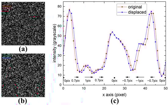
Figure 1.
(a) is a typical speckle pattern from an XST experiment, while (b) is its subpixel deformed counterpart with sinusoidal displacement at a frequency of 0.02 cycle/pixel. (c) shows the positional variation in deformation between (a,b). The red and blue curves in (c) represent intensity profiles along the red line in (a) and blue line in (b), respectively. The arrows beneath indicate the direction and magnitude of displacement between corresponding points, with dots marking positions of profile alignment.
Figure 1a displays a typical speckle pattern from an XST experiment, while Figure 1b shows its subpixel deformed counterpart with sinusoidal displacement at a frequency of 0.02 cycle/pixel. Figure 1c details the positional variation in deformation between Figure 1a,b. The red and blue curves in Figure 1c represent intensity profiles along the red line in Figure 1a and blue line in Figure 1b, respectively. The arrows beneath indicate the direction and magnitude of displacement between corresponding points, with dots marking positions of profile alignment. All displacement vectors collectively form a curve depicting positional displacement between blue and red profiles, as shown by the black curve in Figure 2a. This trigonometric curve has a 50-pixel period (spatial frequency = 0.02 cycle/pixel). The subtle differences between Figure 1a and Figure 1b are detectable only through subpixel registration algorithms, with results indicated by red dots in Figure 2a. Notable discrepancies between measured and actual displacements yield a root mean square error (RMSE) of 0.38. However, detection performance differs significantly for lower-frequency displacements. In Figure 2b, maintaining identical displacement amplitude but extending the period to 500 pixels (frequency = 0.002 cycle/pixel), the measured results (red dots) closely match actual displacements (black curve), achieving a RMSE of 0.01. Thus, different spatial frequencies impose distinct demands on the spatial resolution of subpixel registration algorithms.

Figure 2.
Displacement fields and calculated results of spatial frequencies (a) 0.02 cycle/pixel and (b) 0.002 cycle/pixel. The black curve represents the ground-truth displacement, whereas the red dots denote the results from the peak-finding algorithm.
In speckle-based wavefront measurements, batches of similar optics generate displacement fields with comparable spatial spectra. While these spectra are spread broadly, the optimal subpixel registration algorithm and parameters can be selected on the basis of dominant frequencies (e.g., peak or mean frequencies), spatial resolution, speckle size, and pixel size.
Thus, spatial resolution is a critical metric for subpixel registration algorithms in XST experiments. Existing evaluation methods fail to guide algorithm selection in such scenarios. This study addresses this gap by proposing a comprehensive evaluation method that incorporates displacement accuracy and spatial resolution, also compares the performances of peak-finding and iterative spatial domain cross-correlation algorithms.
2. Methods
To evaluate the spatial resolution of subpixel registration algorithms and guide the appropriate selection of algorithms for practical measurement, this method draws inspiration from the concept of the modulation transfer function (MTF) and uses the RMSE of the subpixel registration as a function of the spatial frequency as the evaluation criterion. In optics, the MTF is defined as the ratio of the relative image contrast to the relative object contrast, which quantifies the system’s ability to preserve spatial details, i.e., its response to varying spatial frequencies. The MTF curve is typically normalized to 1 at zero spatial frequency and gradually decreases as the spatial frequency increases until it reaches zero. A contrast of zero indicates the complete loss of image detail. Spatial resolution describes the ability of an imaging system to resolve detail in the object that is being imaged. Thus, one critical role of the MTF is to reflect the spatial resolution of an optical system. Since this study aims to evaluate subpixel registration algorithms, including their spatial resolution capabilities, adopting an MTF-like evaluation framework is appropriate.
The core of this method involves generating a series of reference–sample image pairs with periodic displacement fields of varying spatial frequencies. The subpixel registration algorithms under evaluation are applied to compute displacement fields for these image pairs. The RMSE between the computed displacement fields and the predefined ground-truth displacements serves as the accuracy metric for each spatial frequency. The RMSE curve across spatial frequencies is then used as the overall performance criterion. In the MTF framework, the optical system’s response capability varies with spatial frequency, where higher values are preferable. In contrast, this method focuses on minimizing the RMSE between the computed and true displacements as the spatial frequency changes, where lower values indicate superior performance.
In addition to the spatial frequency, the speckle size and subset size influence the results. These factors are addressed differently in this method.
In practical measurements, speckle size is determined by parameters such as source coherence, speckle generator properties, and detector performance, which are typically fixed during data analysis. Therefore, this study categorizes the results on the basis of their distinct speckle sizes. As shown in Section 3, the speckle size has an impact on accuracy but is smaller than the spatial frequency and subset size.
For subset size selection, two factors are prioritized. On the one hand, larger subsets encompass more data, improving the similarity criteria and displacement measurement accuracy. On the other hand, larger subsets aggregate displacement measurements over broader regions, degrading spatial resolution. In scenarios involving pure translation between reference and sample images, larger subsets yield better displacement accuracy. However, for periodically varying displacement fields, these factors interact, resulting in an optimal subset size that minimizes measurement inaccuracies. This study selects the optimal subset size for each scenario as the basis for evaluation.
As noted earlier, the evaluation requires generating image pairs with predefined displacement fields. Section 2.1 details the methodology for generating such image pairs and modulating key parameters of speckle patterns. This work also evaluates and compares two widely used algorithms—the peak-finding algorithm and the iterative spatial domain cross-correlation algorithm—under the proposed framework. Section 2.2 and Section 2.3 provide concise descriptions of these algorithms.
2.1. Speckle Generation
To precisely control parameters such as displacement fields and speckle sizes, this study employs a computational program to generate reference–sample image pairs. On the basis of the intensity and spatial distribution characteristics of X-ray near-field speckle patterns, a mathematical model is constructed, and speckle images are synthesized by integrating the model with random number generation. The model in Reference [12] is adopted to simulate speckles:
where Ir is the reference image, and Is is the deformed sample image. The parameter n represents the number of speckles, the intensity profile of individual speckles along the x-direction is illustrated in Figure 3, Ik represents the randomly assigned peak intensity of each speckle, xk and yk are the randomly distributed positions of individual speckles, u and v define the displacements of the individual speckles, and R is the width of the speckle at the height of e−1·Ik. For the entire speckle pattern, the speckle size is determined using the autocorrelation function (ACF). The full-width half maximum of the central peak of ACF curve is employed as speckle size for it is stable and objective. By sampling this continuous distribution on a grid aligned with the detector pixel array, speckle images resembling experimental results are generated. Since the distribution is defined by continuous functions, it allows for modulations such as translation, rotation, and deformation, producing corresponding reference and sample image pairs.
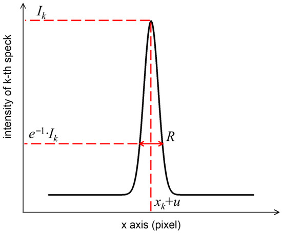
Figure 3.
Intensity profile of k-th individual speckle along the x-direction. Ik represents the randomly assigned peak intensity of each speckle, xk is the randomly distributed position of the individual speckle, u defines the displacement of the individual speckle, and R is the width of the individual speckle at the height of e−1·Ik.
For this study, the sample image is modulated by introducing a displacement field that varies sinusoidally, meaning that the displacement between the sample and reference images exhibits periodic spatial variation. The frequency of the displacement field can be freely adjusted. To align with subpixel registration objectives, the amplitude of the displacement field is set to 1 pixel.
To accurately generate speckle patterns of the desired sizes, the relationships between the speckle size and model parameters are investigated. Using the control variate method, speckle images are generated with varying parameters, and the relationships between speckle size and these parameters are analyzed, as illustrated in Figure 4.
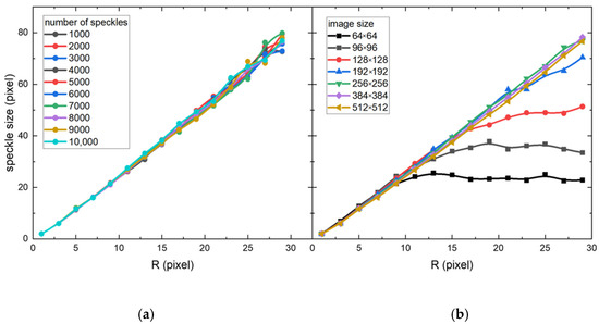
Figure 4.
Trends in speckle size variation with model parameters. (a): Speckle size scales linearly with R, independent of n. (b): Speckle size as a function of R and image size.
Figure 4a reveals that the speckle size scales linearly with R, independent of n. Figure 4b indicates that the linear regime is limited; beyond this range, the speckle size remains nearly constant (or saturated). The extent of the linear regime and the saturated speckle size are governed primarily by the image size. As this topic falls outside the scope of this study, further analysis is omitted. A 512 × 512 image size, offering best linearity and the broadest linear range, is selected to generate speckle patterns on the basis of linear fitting results. Validation confirms that the parameters of the generated speckle patterns align with expectations.
Based on the aforementioned model and parameters, the authors generated a set of speckle images using Python 3.11.9 programming. This dataset includes reference images with speckle sizes ranging from 10 to 50 pixels (in steps of 5 pixels), along with corresponding sample images featuring identical speckle sizes and displacement periods (1/f) ranging from 100 to 500 pixels/cycle (in steps of 50 pixels/cycle). In total, 162 images were produced (provided in Supplementary Materials) for subsequent algorithm evaluation.
2.2. Peak-Finding Algorithm
The peak-finding algorithm assumes that the similarity follows a peak-shaped distribution. To localize the subpixel displacement, surface fitting is performed on discrete pixel-corresponding points, a continuous similarity distribution is reconstructed, and the peak position between discrete pixels is identified. This technique is an efficient and easily implementable subpixel registration method. In this work, a simplified approach using Taylor expansion and the zero-derivative property at the peak is adopted to increase computational efficiency [19]. Specifically, a second-order Taylor expansion is applied to the discrete similarity distribution around its highest point (x0, y0), as expressed in Equation (2):
where L(x, y) represents the hypothesized continuous similarity distribution. At the peak, the first derivatives of the similarity function are 0,
These equations can be rewritten as
Solving these equations yields the subpixel displacements:
The coefficients A, B, C, D, and E are derived directly from partial derivatives of the similarity function, which can be efficiently computed via differences. The peak-finding algorithm program used in this study was developed by the authors using Python 3.11.9.
2.3. Iterative Spatial Domain Cross-Correlation Algorithm
The iterative spatial domain cross-correlation algorithm assumes that each point in the reference image can be mapped to a corresponding point in the sample image, where the rectangular subset containing the reference point may undergo stretching or compression in the sample image. Consequently, the displacement between two points comprises the distance between subset centers, normal strain terms, shear strain terms, and rotation terms, with the latter three arising from deformation. These components collectively form a vector P, and the similarity criterion, i.e., the correlation coefficient C between undeformed and deformed subsets, is defined as a function of P. When the similarity between the computed subset and the target subset is maximized, the correlation coefficient C reaches its extremum. Solving for the vector P corresponding to this extremum yields the displacement, which is typically achieved via the Newton‒Raphson iteration method or the Levenberg‒Marquardt algorithm. The integer-pixel search result serves as the first initial guess for iteration, leading to
where Pi is the initial guess, Pi+1 is the iteratively refined approximation, ∇C(Pi) is the gradient of the correlation function, and ∇∇C(Pi) is the second-order derivative (Hessian matrix) of the correlation function.
Digital images lack grayscale information between pixels, necessitating subpixel grayscale values and gradients for iterative computations. Interpolation methods are employed to estimate subpixel data, making the choice of interpolation scheme critical for computational accuracy and convergence behavior. A bicubic spline interpolation scheme ensures the continuity and smoothness of grayscale intensities and their first-order spatial derivatives, demonstrating high registration accuracy and robust convergence properties.
The iterative spatial domain cross-correlation algorithm employed in this study was obtained from Reference [20], which is widely recognized in the field. While the computational principles align with the Newton-Raphson iteration method, the program incorporates the inverse compositional (IC) approach to avoid redundant Hessian matrix calculations and approximates the Hessian via the Gauss‒Newton (GN) method. This strategy, termed the IC-GN, significantly reduces computational complexity while maintaining accuracy. Hereafter, the term “IC-GN algorithm” will be used in place of “iterative spatial domain cross-correlation algorithm.”
3. Results
Notably, the subset size significantly impacts the computational results. Thus, this study first investigates trends in computational outcomes across varying subset sizes under different conditions to identify the subset size that minimizes the RMSE. A subset with this optimal size is termed the “optimal subset”, and the corresponding minimum RMSE is defined as the “optimal RMSE”. The curve of optimal RMSE as a function of spatial frequency serves as the basis for evaluating spatial resolution. Following this workflow, both the peak-finding algorithm and the IC-GN algorithm are analyzed, and the results are detailed below.
3.1. Peak-Finding Algorithm
The RMSE versus the subset size from speckle image pairs of different speckle size was calculated, and it is found that the trends of the RMSE versus the subset size differ between conditions with and without periodic displacement fields. An example of speckle image pairs with a speckle size of 30 pixels is illustrated in Figure 5. In the absence of periodic displacement fields, the RMSE decreases approximately inversely with increasing subset size. For the periodic displacement fields (100-pixel period), the RMSE decreases with the subset size smaller than 15 pixels, and increases with the subset size larger than 15 pixels. This divergence arises because the former case is governed solely by the data volume within the subset, whereas the latter involves a trade-off between the data volume and spatial resolution.
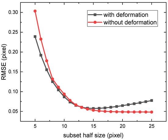
Figure 5.
Comparison of peak-finding algorithm error trends under periodic and nonperiodic displacement fields. A pair of speckle images with a speckle size of 30 pixels is used. In the absence of periodic displacement fields, the RMSE decreases approximately inversely with increasing subset size. For the periodic displacement fields (100-pixel period), the RMSE initially decreases and then increases with subset size.
For the periodic displacement fields of varying spatial frequencies from 0.002 cycle/pixel to 0.01 cycle/pixel, the RMSE exhibit similar trends (Figure 6). For all frequencies, the RMSE first decreases and then increases with the subset size. The lower-frequency curves resemble those of the nonperiodic case because low-frequency displacements vary gradually with position, maintaining accuracy even with larger subsets, so their RMSE is primarily determined by data volume (i.e., subset size). The higher-frequency curves show steeper variations, underscoring the criticality of subset selection. This is because high-frequency displacements change rapidly with position. When the subset size approaches the displacement period scale, different regions within the subset reflect varying displacements, and their averaging effect fails to represent the central displacement accurately. Consequently, the RMSE is jointly influenced by data volume (subset size) and displacement frequency, with higher frequencies exerting greater impact on RMSE, ultimately leading to smaller optimal subsets.
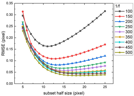
Figure 6.
Peak-finding algorithm error trends for displacement fields of varying spatial frequencies (from 0.002 cycle/pixel to 0.01 cycle/pixel) across subset sizes. For all frequencies, the RMSE first decreases and then increases with the subset size.
Even with optimal subset selection, the optimal RMSE for low-frequency displacement fields remain significantly smaller than those for high-frequency cases (Figure 6). This discrepancy is correlated with frequency-dependent optimal subset sizes (Figure 7). For clarity, Figure 7 uses 1/f as the horizontal axis. The optimal subset size exhibits a linear relationship with 1/f. Specific fitting parameters are provided in Table 1 and Table 2 of Section 3. As the spatial frequency increases, the spatial resolution requirements escalate, necessitating smaller subsets. Consequently, the data volume decreases and optimal RMSE increases accordingly.
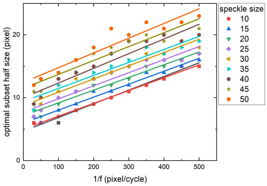

Table 1.
Fitting parameters for the linear relationship between optimal subset sizes and 1/f across different speckle sizes for both algorithms, along with their mean values and relative standard deviations (RSD).
Table 2.
Fitting parameters for the linear relationship between optimal RMSE and 1/f (both on logarithmic axes) across different speckle sizes for both algorithms, along with their mean values and relative standard deviations.
Figure 8 shows the optimal RMSE for all speckle sizes and spatial frequencies, which are plotted on logarithmic axes. The optimal RMSE grow exponentially (detailed fitting parameters are available in Table 1 and Table 2 of Section 3) with spatial frequency (1–2 orders of magnitude within the region of interest) and weakly with speckle size (<1 order of magnitude), confirming that spatial frequency dominates over speckle size in influencing accuracy, and reflecting the heightened spatial resolution demands for high-frequency displacement measurements.
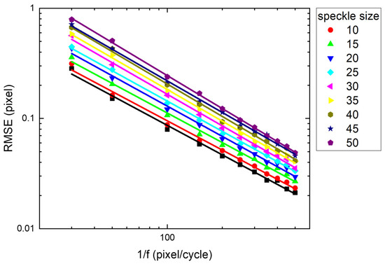
Figure 8.
Optimal RMSE for the peak-finding algorithm across 1/f and speckle sizes. The optimal RMSE grow exponentially (detailed fitting parameters are available in Table 1 and Table 2) with spatial frequency (1–2 orders of magnitude within the region of interest) and weakly with speckle size (<1 order of magnitude).
3.2. Iterative Spatial Domain Cross-Correlation (IC-GN) Algorithm
For comparison with the peak-finding algorithm, the IC-GN algorithm is also analyzed using speckle images with a speckle size of 30 pixels. Figure 9 shows the RMSE trends under periodic and nonperiodic displacement fields. Without periodic displacement, the RMSE decreases inversely with the subset size. For periodic displacement (100-pixel period), the RMSE decreases with subsets smaller than 29 pixels and then increases with subsets larger than 29 pixels, mirroring the peak-finding algorithm’s behavior and rationale. Evidently, the optimal subset size for IC-GN is significantly larger than that for the peak-finding algorithm. This occurs because Equation (6) in IC-GN requires more data to achieve reliable solutions, resulting in a slower decrease in RMSE with increasing subset size compared to the peak-finding algorithm. While spatial frequency affects both algorithms similarly, the combined effect leads IC-GN to require larger subsets to reach optimal RMSE values.
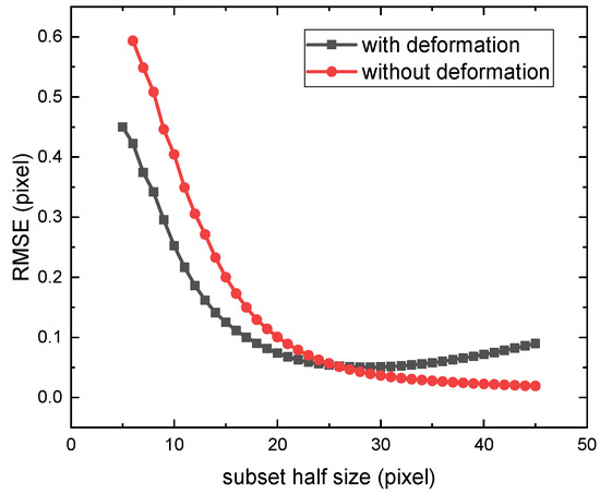
Figure 9.
Comparison of IC-GN algorithm error trends under periodic and nonperiodic displacement fields. Without periodic displacement, the RMSE decreases inversely with the subset size. For periodic displacement (100-pixel period), the RMSE first decreases and then increases with subset size, mirroring the peak-finding algorithm’s behavior and rationale.
For displacement fields of varying spatial frequencies, the RMSE trends align with those of the peak-finding algorithm (Figure 10). Lower frequencies approximate nonperiodic cases, whereas higher frequencies exhibit sharper sensitivity to the subset size, again highlighting spatial resolution demands. Similarly to the peak-finding algorithm, the optimal RMSE for low-frequency fields are smaller than those for high-frequency fields. Compared to the peak-finding algorithm, IC-GN exhibits more clustered RMSE curves across different frequencies. The influence of spatial frequency becomes apparent only as the subset size approaches the optimum, where the curves begin to diverge. This further demonstrates IC-GN’s stronger dependence on data volume—when data is insufficient, its errors are large enough to overshadow the effects of spatial frequency.
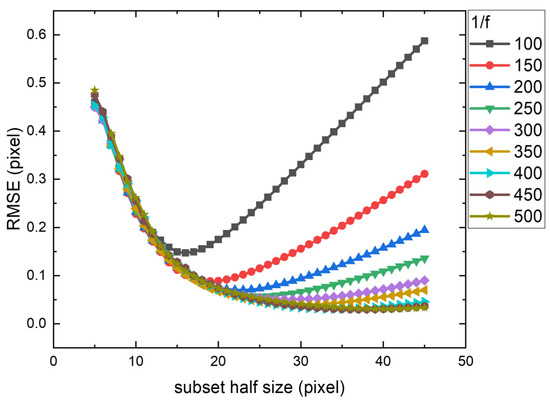
Figure 10.
IC-GN algorithm error trends for displacement fields of varying spatial frequencies (from 0.002 cycle/pixel to 0.01 cycle/pixel) across subset sizes. For all frequencies, the RMSE trends align with those of the peak-finding algorithm. Compared to the peak-finding algorithm, IC-GN exhibits more clustered RMSE curves across different frequencies.
Figure 11 illustrates the optimal subset sizes across parameters. The optimal subset size shows a linear relationship with 1/f. Detailed fitting parameters are provided in Table 1 and Table 2 of Section 3. Figure 11 also shows that higher spatial frequencies demand smaller subsets, decreasing the data volume and increasing optimal RMSE.
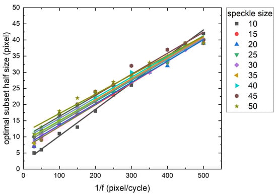
Figure 12 aggregates the optimal RMSE for all speckle sizes and spatial frequencies. On logarithmic axes, optimal RMSE exhibit exponential growth (Detailed fitting parameters are provided in Table 1 and Table 2 of Section 3) with spatial frequency (1–2 orders of magnitude within the region of interest) but remain nearly independent of speckle size, contrasting sharply with the peak-finding algorithm.
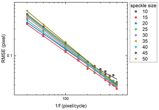
Figure 12.
Optimal RMSE for the IC-GN algorithm across 1/f and speckle sizes. Optimal RMSE exhibit exponential growth (Detailed fitting parameters are provided in Table 1 and Table 2) with spatial frequency (1–2 orders of magnitude within the region of interest) but remain nearly independent of speckle size, contrasting sharply with the peak-finding algorithm.
4. Discussion and Comparison
The peak-finding algorithm operates on the principle that similarity between speckle images follows a unimodal distribution in the XY plane, with peak position indicating subpixel displacement. It employs straightforward algebraic computations to locate this peak. In contrast, the IC-GN algorithm extends beyond mere translation by incorporating rotational and deformation parameters, assuming a unimodal similarity distribution in a six-dimensional space where the peak corresponds to subpixel displacement, rotation, and deformation. This method utilizes iterative procedures and interpolation for peak localization.
While IC-GN employs more sophisticated models and computational approaches by accounting for additional parameters, it simultaneously demands substantially larger input data to achieve reliable performance. Traditional evaluation methods focusing solely on translation impose no constraints on data volume, thus favoring IC-GN’s performance. However, when spatial resolution becomes an evaluation criterion, significant limitations emerge regarding data requirements. Larger data volumes necessitate larger subsets, which inevitably lead to loss of detail and compromised spatial resolution. Consequently, under the spatial-resolution-aware evaluation framework proposed in this study, IC-GN no longer maintains absolute superiority over the peak-finding algorithm, with each algorithm demonstrating distinct advantages in specific scenarios.
Analyzing spatial frequency constraints on data requirements reveals fundamental differences. Without spatial frequency considerations, both algorithms benefit from larger subsets. However, incorporating spatial frequency introduces a trade-off: excessively large subsets cause detail loss, necessitating balanced subset selection between data volume and spatial resolution. Higher spatial frequencies, carrying richer detail, impose stricter constraints on subset sizes. This optimal balance is quantified through optimal subset sizes, with both algorithms sharing similar trends in optimal subset size variation as shown in Figure 13.
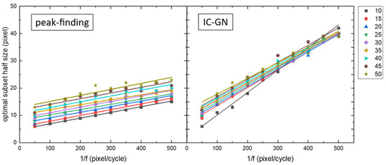
Figure 13.
Comparison of optimal subset sizes between the peak-finding and IC-GN algorithms. The optimal subset sizes for both methods increase linearly with 1/f, but the IC-GN algorithm exhibits a steeper rate of increase.
The optimal subset sizes for both methods increase linearly with 1/f, but the IC-GN algorithm exhibits a steeper rate of increase. Linear fitting results in Table 1 show the peak-finding algorithm’s average slope is 0.02141 versus 0.06520 for the IC-GN algorithm—approximately three times steeper. This indicates that at low frequencies, the IC-GN algorithm requires substantially more data than the peak-finding algorithm to achieve target performance. At high frequencies (approximately 0.01), spatial resolution becomes the dominant constraint, forcing both algorithms toward similar subset size levels. In most cases, the IC-GN algorithm requires larger optimal subset sizes than the peak-finding algorithm, partially explaining the latter’s faster computational speed.
Table 1 further reveals that both algorithms exhibit significantly larger RSD in fitting intercepts than in slopes. This occurs because intercepts reflect speckle size influence on subsets while slopes represent spatial frequency effects—two independent factors. The consistent increase in fitting intercepts with speckle size for both algorithms indicates reduced information per unit area with larger speckles, necessitating larger subsets to maintain accuracy.
Figure 14 illustrates the influence of spatial frequency on the accuracy of both algorithms. Figure 14 uses 1/f as the horizontal axis and RMSE as the vertical axis, where higher RMSE values indicate poorer accuracy. The red and blue lines represent fitting results for the peak-finding algorithm and IC-GN, respectively, with detailed parameters provided in Table 2. From Figure 14, it can be observed that within the tested range, the optimal RMSE of both methods are comparable. Data in Table 2 shows average slopes of −0.9369 and −0.9883, and average intercepts of 1.076 and 1.126, respectively, indicating small difference in overall accuracy between the two algorithms, and the difference between the two algorithms is significantly smaller than those obtained via traditional methods.
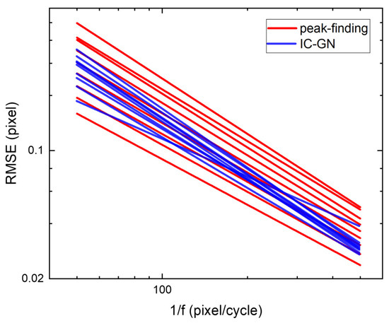
Figure 14.
Comparison of the optimal RMSE between the peak-finding and IC-GN algorithms. The optimal RMSE of both methods are comparable, and the difference is significantly smaller than those obtained via traditional methods.
The slopes in Table 2 reflect the influence of spatial frequency, while the intercepts represent the effect of speckle size. Both algorithms exhibit large RSD in fitting intercepts, indicating that RMSE is affected by speckle size. As speckle size increases, both intercept and RMSE values rise, leading to degraded accuracy. The underlying reason aligns with the explanation for optimal subset sizes: increased speckle size reduces information density, thereby diminishing accuracy.
At high spatial frequencies (>0.01 cycle/pixel approximately), the optimal RMSE for both algorithms are excessively large (>0.1 pixel), rendering them impractical for experimental measurement. This occurs because the optimal RMSE for both algorithms exhibit exponential dependence on the spatial frequency, causing accuracy to rapidly degrade to unacceptable levels when spatial frequency exceeds a certain threshold.
At low spatial frequencies (<0.01 cycle/pixel approximately), the optimal RMSE for the peak-finding algorithm increase noticeably with speckle size, whereas those for the IC-GN algorithm are less influenced by speckle size. Consequently, in the low-frequency region, for larger speckle sizes (>30 pixels), the IC-GN algorithm outperforms the peak-finding algorithm, whereas the latter excels for smaller speckle sizes (<15 pixels). Traditional evaluations under ideal translational conditions favor the IC-GN algorithm, but this study reveals that both algorithms exhibit distinct advantages across different spatial frequency and speckle size regimes when spatial resolution is considered.
5. Conclusions
To comprehensively and accurately evaluate the performance of subpixel registration algorithms, this study develops a novel evaluation method that incorporates the influence of the displacement field spatial frequency on the registration accuracy. The optimal RMSE between the computed and ground-truth displacements, plotted as a function of spatial frequency, serves as the primary metric for assessing spatial resolution. An analysis of the RMSE trends reveals that, under periodic displacement fields, both algorithms exhibit a U-shaped relationship between the RMSE and the subset size, with a distinct optimal subset minimizing error. This pattern results from the combined effects of data volume and spatial frequency on algorithm performance. The performance difference between the two algorithms primarily stems from IC-GN’s requirement for more input data than the peak-finding algorithm to achieve comparable accuracy.
At high spatial frequencies, the stringent spatial resolution requirements lead to very small optimal subsets, resulting in insufficient data volume for both algorithms. Neither algorithm is practical because of the excessive RMSE. At low spatial frequencies (<0.01 cycle/pixel approximately), the peak-finding algorithm outperforms the IC-GN for small speckle sizes (<15 pixels), while the latter excels for larger speckles (>30 pixels). This conclusion strongly contrasts with traditional evaluations based on ideal translational conditions. These findings underscore the necessity of incorporating spatial resolution and speckle size into algorithm selection criteria for practical applications, particularly in X-ray near-field speckle wavefront measurements.
Supplementary Materials
The following supporting information can be downloaded at: https://www.mdpi.com/article/10.3390/opt6040054/s1, Produced Speckle Images: raw speckle data; Original Data S1: speckle production analysis.xlsx; Original Data S2: peakfinding data analysis.xlsx; Original Data S3: ncorr data analysis.xlsx.
Author Contributions
Conceptualization, F.L.; Funding acquisition, F.L.; Methodology, F.L. and J.Y.; Project administration, F.L.; Software, J.Y.; Validation, J.Y., H.Z. and P.W.; Visualization, H.Z. and P.W.; Writing—original draft, F.L.; Writing—review & editing, J.Y., H.Z. and P.W. All authors have read and agreed to the published version of the manuscript.
Funding
This research was funded by the National Natural Science Foundation of China, grant number 12305367.
Data Availability Statement
The original contributions presented in this study are included in the article/Supplementary Materials. Further inquiries can be directed to the corresponding author.
Acknowledgments
This work was supported by HEPS test beamline.
Conflicts of Interest
The authors declare no conflicts of interest.
Abbreviations
The following abbreviations are used in this manuscript:
| XST | X-ray speckle tracking |
| DIC | digital image correlation |
| MTF | modulation transfer function |
| RMSE | root mean square error |
| ACF | autocorrelation function |
| IC | inverse compositional |
| GN | Gauss‒Newton |
| RSD | relative standard deviation |
References
- Bérujon, S.; Ziegler, E.; Cerbino, R.; Peverini, L. Two-Dimensional X-Ray Beam Phase Sensing. Phys. Rev. Lett. 2012, 108, 158102. [Google Scholar] [CrossRef] [PubMed]
- Wang, H.; Kashyap, Y.; Sawhney, K. From synchrotron radiation to lab source: Advanced speckle-based X-ray imaging using abrasive paper. Sci. Rep. 2016, 6, 20476. [Google Scholar] [CrossRef]
- Zdora, M.-C. State of the Art of X-ray Speckle-Based Phase-Contrast and Dark-Field Imaging. J. Imaging 2018, 4, 60. [Google Scholar] [CrossRef]
- Li, F.; Kang, L.; Yang, F.G. Present Research Status of X-Ray Near-Field Speckle Based Wavefront Metrology. Acta Opt. Sin. 2022, 42, 0800002. [Google Scholar]
- Berujon, S.; Cojocaru, R.; Piault, P.; Celestre, R.; Roth, T.; Barrett, R.; Ziegler, E. X-ray optics and beam characterization using random modulation: Theory. J. Synchrotron Radiat. 2020, 27, 284–292. [Google Scholar] [CrossRef] [PubMed]
- Berujon, S.; Cojocaru, R.; Piault, P.; Celestre, R.; Roth, T.; Barrett, R.; Ziegler, E. X-ray optics and beam characterization using random modulation: Experiments. J. Synchrotron Radiat. 2020, 27, 293–304. [Google Scholar] [CrossRef] [PubMed]
- Pan, B. Digital image correlation for surface deformation measurement: Historical developments, recent advances and future goals. Meas. Sci. Technol. 2018, 29, 082001. [Google Scholar] [CrossRef]
- Pan, B.; Qian, K.; Xie, H.; Asundi, A. Two-dimensional digital image correlation for in-plane displacement and strain measurement: A review. Meas. Sci. Technol. 2009, 20, 062001. [Google Scholar] [CrossRef]
- Zhang, Z.-F.; Kang, Y.-L.; Wang, H.-W.; Qin, Q.-H.; Qiu, Y.; Li, X.-Q. A novel coarse-fine search scheme for digital image correlation method. Measurement 2006, 39, 710–718. [Google Scholar] [CrossRef]
- Guizar-Sicairos, M.; Thurman, S.T.; Fienup, J.R. Efficient subpixel image registration algorithms. Opt. Lett. 2008, 33, 156–158. [Google Scholar] [CrossRef] [PubMed]
- Xie, J.; Mo, F.; Yang, C.; Li, P.; Tian, S. A novel sub-pixel matching algorithm based on phase correlation using peak calculation. Int. Arch. Photogramm. Remote Sens. Spatial Inf. Sci. 2016, 41, 253–257. [Google Scholar] [CrossRef]
- Bing, P.; Hui-Min, X.; Bo-Qin, X.; Fu-Long, D. Performance of sub-pixel registration algorithms in digital image correlation. Meas. Sci. Technol. 2006, 17, 1615–1621. [Google Scholar] [CrossRef]
- Ping, L.; Jiangang, Z.; Gang, L.; Bin, H.; Zhipeng, W.; Yanmin, Z.; Bo, L. Research on Performance of Sub-pixel Displacement Measurement Algorithm. In Proceedings of the 2021 IEEE 2nd International Conference on Big Data, Artificial Intelligence and Internet of Things Engineering (ICBAIE), Nanchang, China, 26–28 March 2021; pp. 32–36. [Google Scholar]
- Xiong, L.; Liu, X.; Liu, G.; Liu, J.; Yang, X.; Tan, Q. Evaluation of sub-pixel displacement measurement algorithms in digital image correlation. In Proceedings of the 2011 International Conference on Mechatronic Science, Electric Engineering and Computer (MEC), Jilin, China, 19–22 August 2011. [Google Scholar]
- Li, J.; Peng, Q.; Fan, Z. A Survey of Sub pixel Image Registration Methods. J. Image Graph. 2008, 13, 2070–2075. [Google Scholar]
- Pan, B.; Xie, H.; Dai, F. An investigation of sub-pixel displacements registration algorithms in digital image correlation. Chin. J. Theor. Appl. Mech. 2007, 39, 8. Available online: https://lxxb.cstam.org.cn/en/article/doi/10.6052/0459-1879-2007-2-2006-053 (accessed on 14 October 2025).
- Pan, B.; Xie, H.; Wang, Z.; Qian, K.; Wang, Z. Study on subset size selection in digital image correlation for speckle patterns. Opt. Express 2008, 16, 7037–7048. [Google Scholar] [CrossRef] [PubMed]
- Tian, N.; Jiang, H.; Li, A.; Liang, D.; Yu, F. High-precision speckle-tracking X-ray imaging with adaptive subset size choices. Sci. Rep. 2020, 10, 14238. [Google Scholar] [CrossRef] [PubMed]
- Matthew Brown, D.L. Invariant Features from Interest Point Groups. In Proceedings of the British Machine Vision Conference, Cardiff, UK, 2–5 September 2002; BMVA Press: Durham, UK. [Google Scholar]
- Blaber, J.; Adair, B.; Antoniou, A. Ncorr: Open-Source 2D Digital Image Correlation Matlab Software. Exp. Mech. 2015, 55, 1105–1122. [Google Scholar] [CrossRef]
Disclaimer/Publisher’s Note: The statements, opinions and data contained in all publications are solely those of the individual author(s) and contributor(s) and not of MDPI and/or the editor(s). MDPI and/or the editor(s) disclaim responsibility for any injury to people or property resulting from any ideas, methods, instructions or products referred to in the content. |
© 2025 by the authors. Licensee MDPI, Basel, Switzerland. This article is an open access article distributed under the terms and conditions of the Creative Commons Attribution (CC BY) license (https://creativecommons.org/licenses/by/4.0/).