Abstract
Quadcolor cameras with conventional RGB channels were studied. The fourth channel was designed to improve the estimation of the spectral reflectance and chromaticity from the camera signals. The RGB channels of the quadcolor cameras considered were assumed to be the same as those of the Nikon D5100 camera. The fourth channel was assumed to be a silicon sensor with an optical filter (band-pass filter or notch filter). The optical filter was optimized to minimize a cost function consisting of the spectral reflectance error and the weighted chromaticity error, where the weighting factor controls the contribution of the chromaticity error. The study found that using a notch filter is more effective than a band-pass filter in reducing both the mean reflectance error and the chromaticity error. The reason is that the notch filter (1) improves the fit of the quadcolor camera sensitivities to the color matching functions and (2) provides sensitivity in the wavelength region where the sensitivities of RGB channels are small. Munsell color chips under illuminant D65 were used as samples. Compared with the case without the filter, the mean spectral reflectance rms error and the mean color difference (ΔE00) using the quadcolor camera with the optimized notch filter reduced from 0.00928 and 0.3062 to 0.0078 and 0.2085, respectively; compared with the case of using the D5100 camera, these two mean metrics reduced by 56.3%.
1. Introduction
Traditional tricolor cameras are equipped with red, green, and blue channels, which are used to capture long-wavelength, medium-wavelength, and short-wavelength image signals, respectively. This RGB camera can not only capture color images but also recover surface spectral reflectance pixel by pixel. Spectral reflectance images have broad application prospects in the fields of color reproduction, medical diagnosis, agricultural detection, and remote sensing [1,2,3,4,5,6,7,8,9,10]. Using cameras to measure spectral reflectance has the advantages of fast measurement speed, high pixel resolution, low cost, and a small form factor [11,12,13,14], compared with imaging spectrometers [15,16]. Therefore, the application potential of cameras is high.
However, the disadvantage of using a camera is its measurement accuracy, since the spectral reflectance is estimated from the camera signal. The sensitivity spectrum of conventional cameras ranges from 400 nm to 700 nm due to the presence of an infrared-cut (IR-cut) filter. Conventional cameras usually use an IR-cut filter to filter out long-wave light. Since infrared is not visible, filtering can significantly improve the accuracy of camera color calibration. Using an RGB camera, the estimation maps the 3D signal to a 31D spectrum with a sampling wavelength interval of 10 nm. This estimation method requires a set of training/reference samples to calculate the model parameters. The sample set can be prepared according to a specific application. In addition, using image recognition technology to identify the target of the field application, an estimation method with a suitable sample set can be selected to improve accuracy.
Studies have shown that the accuracy of spectral reflectance estimation can be improved by using a quadcolor camera that maps the 4D signal to a 31D spectrum [17,18]. Figure 1a shows the Bayer color filter array (CFA) for a conventional RGB camera, in which a unit cell contains one red, two green, and one blue square filter. This arrangement has the advantage of high spatial resolution. A quadcolor camera uses a modified CFA without sacrificing spatial resolution, as shown in Figure 1b, where a fourth color filter (labeled “Q”) replaces one of the green filters.
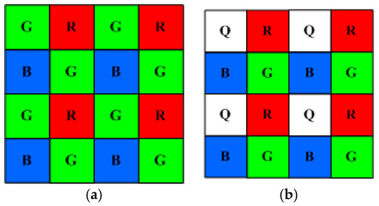
Figure 1.
Color imaging using two different techniques: (a) Bayer color filter array and (b) modified Bayer color filter array. Adapted from [18].
References [17,18] studied a quadcolor camera whose 4th channel has no color filter and whose spectral sensitivities of RGB channels are the same as those of Nikon D5100. The spectral sensitivity of the 4th channel is the product of the sensitivity of the silicon image sensor and the transmittance of the IR-cut filter. This quadcolor camera was called RGBF camera, where the 4th channel was called the F-channel because it was color-filter-free. In [18], the mean root-mean-square (RMS) error of spectral reflectance (ERef) and the color difference (ΔE00) of the test samples reduced from 0.01785 and 0.4778 using D5100 to 0.00928 and 0.3062 using the RGBF camera, respectively. The objective of this article is to investigate the filter design for the 4th channel to further improve the accuracy of spectral reflectance and chromaticity estimation.
Many estimation methods have been proposed for spectral reflectance recovery, which are based on basis spectra [19,20,21,22], Wiener estimation [12,23,24], regression [25,26,27,28,29,30,31,32], and interpolation [17,18,33,34,35,36,37]. Except for the basis-spectrum method, these methods have the problem of irradiance dependence, i.e., the spectral shape of the estimated reflectance depends on the irradiance of the object surface. As mentioned above, it requires a sample set that is prepared under illuminants. However, the irradiance on the object surface may change in field applications.
Reference [18] proposed an irradiance-independent look-up table (II-LUT) method based on interpolation to estimate spectral reflectance. The results showed that the estimation accuracy of the II-LUT method is better than that of the basis-spectrum method. When the interpolation method estimates a sample, it refers to the reference samples adjacent to it in the signal space, while the base spectrum method refers to all training samples even if it uses the weighting technique [20]. Therefore, the II-LUT method has higher accuracy. This article adopts the II-LUT method to recover spectral reflectance.
The 4th channel using a short-pass or long-pass filter was studied in [17], where the traditional irradiance-dependent spectrum reconstruction methods were used. The study showed that the use of short-pass and long-pass filters is beneficial for reducing chromaticity error and reflectance error, respectively. In addition, when either the chromaticity error or the reflectance error decreases, the other error increases. In this article, a cost function consisting of the mean reflectance error and the weighted mean chromaticity error was used for optimizing the filter, where band-pass filters and notch filters were considered. The results show that the use of a notch filter can effectively reduce reflectance and chromaticity errors, but if ultra-low chromaticity errors are desired, using a band-pass filter is better.
This article is organized as follows. Section 2 and Section 3 describe the materials, assessment metrics, and methods, where the assumed color filter spectral transmittance, the optimization cost function, and the II-LUT method are presented in Section 3.1, Section 3.2, and Section 3.3, respectively. Section 4.1 and Section 4.2 present and discuss the results using band-pass optical filters and notch optical filters, respectively. Section 4.3 shows some examples of the recovered spectra. Section 5 provides the conclusions.
2. Materials and Assessment Metrics
2.1. Camera Spectral Sensitivities
By convention, we sampled a spectrum from 400 nm to 700 nm in steps of 10 nm, where the spectrum vector S = [S(400 nm), S(410 nm), …, S(700 nm) ]T and S(λ) is the spectral amplitude at wavelength λ. There are a total of Mw =31 sampling wavelengths.
The RGB channels of the quadcolor camera considered are those of the Nikon D5100 camera [38]. The spectral sensitivity vectors of the three channels and the 4th channel were designated as SCamR, SCamG, SCamB, and SCamQ, respectively. Without the filter specified in Section 3.1, the 4th channel is the F-channel of the RGBF camera considered in [17,18], and its spectral sensitivity vector was designated as SCamF.
2.2. Color Samples
The 1268 matt Munsell color chips under the illuminant D65 were taken as color samples [39]. The same 202 reference/training samples and 1066 test samples in [17,18,37] were adopted.
The reflection spectrum vector from a color chip is
where SRef and SD65 are the spectral reflectance vector of a color chip and the spectrum vector of the illuminant D65, respectively, and the operator is the element-wise product. Reference [37] showed the reference/training samples and test samples in the CIELAB color space, where the CIE 1931 color matching functions (CMFs) were adopted.
The spectral sensitivity vector DCamU and the signal value U of the U channel of the quadcolor camera, where U = R, G, B, and Q, under the white balance condition are
U = SReflectionTDCamU
In Equation (2), SWhite is the spectral reflectance vector of a white card. The same white card in [17,18,37] was taken. The signal vector representing a quadcolor camera was designated as C = [R, G, B, Q]T. Reference [17] showed the reference/training samples and test samples in the signal space of the RGBF camera.
2.3. Assessment Metrics
When the reflection spectrum vector SRec was reconstructed using the II-LUT method, the spectral reflectance vector SRefRec is the vector SRec divided by the vector SD65 element by element. This article used the same metrics as [18] to assess the reconstructed reflection spectrum and the recovered reflectance spectrum. They are the RMS error ERef = ||SRefRec − SRef||2/Mw1/2, where the operation ||·||2 stands for 2-norm; the goodness-of-fit coefficient GFC = ||SRefRecTSRef||2/||SRefRec||2||SRef||2; the CIEDE2000 ΔE00, which measures the color difference between SRec and SReflection; and the spectral comparison index (SCI), which is an index of metamerism [40].
From reconstructed test samples, we calculated the mean μ, standard deviation σ, 50th percentile PC50, 98th percentile PC98, and maximum MAX of the metrics ERef, ΔE00, and SCI, for which smaller values are better; we also calculated the mean μ, standard deviation σ, 50th percentile PC50, RGF99, and minimum MIN of the metric GFC, for which larger values are better. RGF99 is the ratio of good-fit samples with a GFC > 0.99 [37]. The spectral curve shape is well fitted for GFC > 0.99 [36,41].
3. Methods
3.1. Color Filter Spectral Transmittance
Both band-pass optical filters and notch optical filters were considered.
The band-pass filter is a super-Gaussian filter (SGF), whose spectral transmittance was assumed to be
where TS0 is the maximum transmittance; λSGF is the filter peak wavelength; and σW and α are parameters determined by the filter width ΔλF and edge width ΔλE. The filter width is the full width at half maximum transmittance, i.e., TSGF(λSGF + 0.5ΔλF) = 0.5TS0. The edge width ΔλE was defined as the wavelength interval from 0.1TS0 to 0.9TS0. From Equation (4) and the ΔλF and ΔλE definitions, we have
Given the values of ΔλF and ΔλE, the α in Equation (4) is solved from Equation (5), and the parameter σW is
The notch filter is an inverted super-Gaussian filter (ISGF), whose spectral transmittance was assumed to be
where TI0 is the maximum transmittance; λISGF is the central wavelength; and σW and α are parameters determined by the wavelength separation ΔλFS and edge width ΔλE. The wavelength separation ΔλFS is twice the wavelength interval from zero to the half maximum transmittance, i.e., TISGF(λISGF + 0.5ΔλFS) = 0.5TI0. Given the values of ΔλFS and ΔλE, the values of σW and α also can be solved from Equations (5) and (6), except that ΔλF is replaced by ΔλFS. This article assume TS0 = TI0 = 0.96, which will not affect the results.
The spectral sensitivity vector SCamQ = T SCamF, where T is the spectral transmittance vector calculated from either Equation (4) or Equation (7).
3.2. Optimization Cost Function
If only spectral reflectance recovery is desired, the optimization cost function can be set to the mean ERef. However, color reproduction applications require low color differences. Therefore, we consider a cost function defined as follows:
where ERef,μ and ΔE00,μ are the mean ERef and mean ΔE00, respectively; the Lagrange multiplier γ is a weighting factor that controls the contribution of color difference. Since the values of ERef,μ and ΔE00,μ may differ greatly in magnitude, the Lagrange multiplier was chosen logarithmically. γ = 10−p, where the power p was selected from −3 to 0 in steps of 0.05, i.e., 61 Lagrange multipliers were considered.
θ = ERef,μ + γ ΔE00,μ,
For a given value of γ, the case of using an SGF with wavelength λSGF from 400 nm to 700 nm in steps of 10 nm was considered. For each SGF wavelength, the full width ΔλF and the edge width ΔλE were optimized for the minimum cost function. It was found that the cost function exhibits a highly nonlinear relationship with the full width ΔλF and the edge width ΔλE. The optimization used a brute-force grid search method to ensure that the solution was the global minimum. For practical considerations, the ranges of ΔλF and ΔλE were set to 50 nm to 400 nm and 20 nm to 200 nm, respectively. The optimization process for the case of using ISGF is the same as that for using SGF, and the ranges of the wavelength λISGF, the full wavelength separation ΔλFS, and the edge width ΔλE are also the same.
3.3. II-LUT Method
The II-LUT method interpolates a test sample in the normalized signal space, defined as [18]
r = R/(R + G + B + Q),
g = G/(R + G + B + Q),
b = B/(R + G + B + Q).
We designated the normalized signal vector as c = [r, g, b]T. Reference [18] showed the reference/training samples and test samples in the normalized signal space of the RGBF camera. A tetrahedron mesh can be generated from the normalized reference signal vectors.
If the tetrahedron enclosing a normalized test signal vector c is located, the interpolation method assumes that
where ck is the k-th normalized signal vector at the vertices of the tetrahedron, βk is the barycentric coordinate, and
The coefficients βk, k = 1, 2, 3, and 4, are solved from Equations (12) and (13). From [18], we have
where Sk is the k-th reference spectrum for k = 1, 2, 3, and 4; the coefficient
ηk = (R + G + B + F)/(Rk + Gk + Bk + Fk).
In Equation (15), Rk, Gk, Bk, and Fk are the signal values of the k-th reference spectrum.
Since the vectors c and ck in Equation (12) are independent of the irradiance on the object surface, the spectral shape of the reconstructed reflection spectrum vector SRec is independent of the irradiance. The signal values R, G, B, and F increase linearly with the irradiance, and the magnitude of the reconstructed reflection spectrum vector SRec also increases linearly with the irradiance.
In summary, there are five steps to interpolate the test sample using the II-LUT method, where the flow chart is shown in Figure 2.
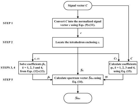
Figure 2.
Flow chart to interpolate the test sample using the II-LUT method.
- STEP 1: Convert the signal vector C of the test sample into the normalized signal vector c.
- STEP 2: Locate the tetrahedron enclosing vector c in the normalized signal space.
- STEP 3: Solve the coefficients βk, k = 1, 2, 3, and 4, from Equations (12) and (13).
- STEP 4: Calculate the coefficients ηk, k = 1, 2, 3, and 4, according to Equation (15).
- STEP 5: Calculate the reconstruction spectrum SRec according to Equation (14).
Due to high saturation, 131 test samples were outside the convex hull of the tetrahedral mesh for the RGBF camera [18]. Since they cannot be interpolated, we extrapolated them using auxiliary reference samples, which are highly saturated samples measured using appropriately selected color filters and reference color chips. This article adopted the same filters and color chips as in [18] so that all test samples could be interpolated/extrapolated using the considered quadcolor cameras.
4. Results and Discussion
4.1. The Use of Band-Pass Optical Filter
Figure 3a shows the mean color difference ΔE00 versus the mean RMS error ERef using the quadcolor cameras with several SGF wavelength λSGF, where the black diamond symbol labeled RGBF indicates that the 4th channel has no color filter. Using the RGBF camera, mean ERef = 0.00928 and mean ΔE00 = 0.3062. As expected, for a given SGF wavelength λSGF, the mean ΔE00 decreases with increasing Lagrange multiplier γ. Although 61 Lagrange multipliers ranging from 10−3 to 1 are selected for each SGF wavelength, the optimized full width ΔλF and edge width ΔλE may be the same or nearly the same for multiple Lagrange multipliers. For example, for λSGF = 550 nm, there are three solution groups, as shown by the green dots in Figure 3a. When γ < 10−2, the performance of the first group is about the same, all close to the RGBF data point. When 10−2 ≤ γ < 10−1.55, the performance of the second group is also about the same, where the mean ERef ≈ 0.01072 and mean ΔE00 ≈ 0.1392. When γ ≥ 10−1.55, the 3rd group has smaller mean ΔE00, but larger mean ERef compared with the 2nd group.
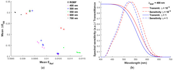
Figure 3.
(a) Mean color difference ΔE00 versus mean RMS error ERef using the quadcolor cameras with the SGF of wavelength λSGF shown in the figure and the Lagrange multiplier γ ranges from 10−3 to 1. The case using the RGBF camera is also shown for comparison. (b) The filter spectral transmittance and spectral sensitivity of the 4th channel for λSGF = 400 nm, where the cases of γ = 10−3 and 1 are shown.
In Figure 3a, the pink dots show the results for λSGF = 400 nm, where the minimum mean ΔE00 is with γ = 1. Since the filter peak wavelength is 400 nm, the SGF is equivalently a short-pass filter in the visible wavelength region. Figure 3b shows the spectral transmittance for λSGF = 400 nm, where γ = 10−3 and 1. The difference between the two cases is not significant. Table 1 shows the full width ΔλF and edge width ΔλE of the two SGFs. The spectral sensitivities using the two SGFs are also shown in Figure 3b, where their peak sensitivities are around 525 nm.

Table 1.
Full width ΔλF and edge width ΔλE of several SGFs. The CMFMisF, mean ΔE00, and mean ERef using D5100, RGBF, and the quadcolor cameras with the filters are shown. The best values of CMFMisF and ΔE00 are shown in bold red. The best value of ERef is shown in bold green.
The blue “+” symbols in Figure 3a indicate the results for λSGF = 500 nm, where the minimum mean ΔE00 is slightly larger than that for λSGF = 400 nm and γ = 1 for both. Such solutions are band-pass filters in the visible wavelength region. Figure 4a is the same as Figure 3a except for λSGF shorter than 500 nm, and the case of λSGF = 400 nm is also shown for comparison. Note that their minimum mean ΔE00 are about the same. In fact, their spectral sensitivities are also about the same. Figure 4b shows the spectral transmittance and spectral sensitivities for λSGF = 480 nm, where γ = 10−3 and 1. Comparing Figure 4b with Figure 3b, although their spectral transmittances are quite different, their spectral sensitivities are similar for the same γ value. The full width ΔλF and edge width ΔλE for λSGF = 480 nm are shown in Table 1. From the spectral sensitivities of γ = 1 shown in the two figures, it can be seen that the peak wavelengths are 520 nm and 525 nm for λSGF = 400 nm and 480 nm, respectively; the full width at half-maximum is about 100 nm in both cases.
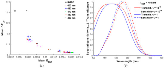
Figure 4.
(a) The same as Figure 3a except for the SGF wavelength λSGF, which is shown in the figure. (b) The filter spectral transmittance and spectral sensitivity of the 4th channel for λSGF = 480 nm, where the cases of γ = 10−3 and 1 are shown.
The mean ΔE00 is related to the CMF mismatch factor (CMFMisF), defined as [17]
for m = x, y, and z. In Equation (17), the operation ||∙||1 is 1-norm, so the relative RMS error σm has the sense of the ratio of standard deviation to the mean; um is the CMF vector, ux = [(λ1), (λ2), …, (λMw)]T, uy = [(λ1), (λ2), …, (λMw)]T, uz = [(λ1), (λ2), …, (λMw)]T, and λj = 400 + (j – 1) × 10 nm for j = 1, 2, …, Mw; uFit is the least squares fit of a CMF vector:
and βR, βG, βB and βQ are the fitting coefficients. The equation for calculating σm in [17] has been corrected to Equation (17).
CMFMisF = (σx2 + σy2 + σz2)1/2,
σm = ||uFit − um||2/|| um||1,
uFit = βRSCamR + βGSCamG + βBSCamB + βQSCamQ,
Figure 5a shows the spectral sensitivities of red, green, blue, and F-channels of the RGBF camera under the white balance condition. Figure 5b shows the least squares fits of the spectral sensitivity vectors of the RGBF camera to the CMF vectors. Figure 6a,b are the same as Figure 5a,b, respectively, except that the filter for λSGF = 480 nm and γ = 1 is applied to the 4th channel. The fits of spectral sensitivities to CMFs shown in Figure 6b are better than those shown in Figure 5b. Table 1 shows the CMFMisF and mean ΔE00 for the cases shown in Figure 3b and Figure 4b, where the results using the D5100 and RGBF cameras are also shown. For the case of λSGF = 400 nm and γ = 1, both the CMFMisF and mean ΔE00 are minimum in the table.
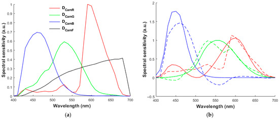
Figure 5.
(a) The spectral sensitivities of red (DCamR), green (DCamG), blue (DCamB), and F (DCamF) channels of the RGBF camera under the white balance condition. (b) Least squares fit of CMF vectors with the spectral sensitivity vectors of the RGBF camera. The CMFs , , and are shown in red, green, and blue, respectively. Solid and dashed lines show the CMFs and least squares fits, respectively. Adapted from [18].
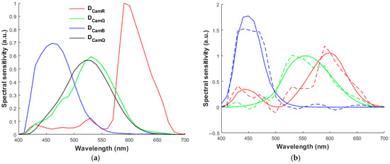
Table 2 shows the assessment metric statistics for the three cases using SGF: (1) λSGF = 480 nm and γ = 10−3, (2) λSGF = 480 nm and γ = 1, and (3) λSGF = 400 nm and γ = 1. We can see that the statistics of the latter two cases are about the same due to the similar spectral sensitivities shown in Figure 3b and Figure 4b. Figure 7a–d show the ERef, GFC, ΔE00, and SCI histograms for the case of λSGF = 480 nm and γ = 1, where the enlarged sub-figures show the distributions of the test samples with worse metric values. The counts of the vertical axis of the figures are the number of samples within the 1066 test samples. The color difference ΔE00 of all test samples using the SGF is less than 1.0, but at the expense of increased spectral reflectance error ERef.
Table 2.
Assessment metric statistics for the spectrum reconstruction of the 1066 test samples using quadcolor cameras. The filter of the 4th camera channel is indicated. The RGBF camera is without a filter. The best values are shown in bold red.
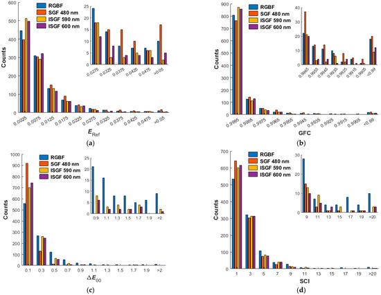
Figure 7.
(a) ERef, (b) GFC, (c) ΔE00, and (d) SCI histograms for the 1066 test samples. The 4th channels of the quadcolor cameras are without a filter (RGBF camera) and with filters. The wavelength of the SGF is λSGF = 480 nm, and the solution of γ = 1 is taken. The wavelengths of the ISGFs are λISGF = 590 nm and 600 nm, where the solutions of γ = 10−3 and 10−1.65 are taken, respectively. The insets show enlarged parts.
From Figure 3a, it can be seen that the mean ERef can be reduced using the filter of long SGF wavelength, e.g., the black dots for 700 nm. The case using the SGF of λSGF = 700 nm and γ = 10−3 has the minimum mean ERef. Figure 8a is the same as Figure 3a, except that SGF wavelengths range from 660 nm to 700 nm in steps of 10 nm. Figure 8b shows the spectral transmittance and spectral sensitivities for the cases of λSGF = 700 nm, where γ = 10−3 and 1. The SGF with λSGF = 700 nm is equivalently a long-pass filter in the visible wavelength region. If a band-pass filter is preferred, Figure 8b also shows the spectral transmittance and spectral sensitivities for λSGF = 680 nm and γ = 10−3. Table 1 gives the full width ΔλF and edge width ΔλE for the cases shown in Figure 8b.
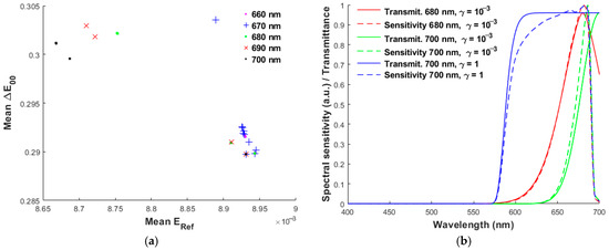
Figure 8.
(a) The same as Figure 3a, except that the SGF wavelength λSGF ranges from 660 nm to 700 nm in steps of 10 nm. (b) The filter spectral transmittance and spectral sensitivity of the 4th channel for λSGF = 680 nm and 700 nm, where their γ values are shown in the figure.
The spectral sensitivities of a commercial tricolor camera, such as D5100, were designed to fit CMFs as closely as possible for color calibration. Due to the characteristics of CMFs, they have low spectral sensitivity in the long-wavelength region. Since the main sensitivity of the 4th channel shown in Figure 8b ranges from 650 nm to 700 nm, the spectral sensitivities of the quadcolor camera cannot fit the CMFs well, and the CMFMisF is larger than that shown in Figure 3b and Figure 4b. Although mean ΔE00 increases, the case of using the long-wavelength SGF has the advantage of a lower mean ERef. The 4th-channel signal can provide a clue of the spectral characteristics of the reflection spectrum in the long-wavelength region for better spectrum reconstruction.
4.2. The Use of Notch Optical Filter
From Section 4.1, we know that although CMFMisF and mean ΔE00 increase, a sensitivity lobe around 685 nm is required to effectively reduce the mean ERef. As will be shown below, in addition to the long-wavelength sensitivity lobe, ISGF can also provide another sensitivity lobe around 500 nm to reduce CMFMisF, thereby reducing both the mean ERef and mean ΔE00.
Figure 9a is the same as Figure 3a, except that ISGF is used. For the visible wavelength region, optical filters with λISGF = 400 nm and 700 nm are equivalently long-pass and short-pass, respectively. The effective notch filter wavelength lies between the two extremes. When λISGF = 550 nm, there is only one solution group with the mean ERef ≈ 0.00832 and mean ΔE00 ≈ 0.2367, which is worse than when using λISGF = 600 nm. The red “x” symbols indicate that using the ISGF with wavelength λISGF = 600 nm can effectively reduce both the mean ERef and mean ΔE00. Figure 9b is the same as Figure 9a, except that λISGF is from 580 nm to 620 nm in steps of 10 nm, where the optimal case is λISGF = 600 nm in green dots for both low mean ERef and mean ΔE00. Figure 10a shows the enlarged plot of the mean ΔE00 versus the mean ERef for λISGF = 600 nm, where the data points of three Lagrange multipliers γ are indicated with the “+” sign. Note that the case of γ = 10−1.65 is the optimal value that represents a trade-off between the mean ERef and the mean ΔE00.
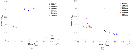
Figure 9.
(a) The same as Figure 3a, except that the quadcolor cameras are with the ISGF. (b) The same as (a), except that the ISGF wavelength λISGF ranges from 580 nm to 620 nm in steps of 10 nm.
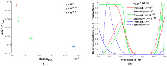
Figure 10.
(a) The same as the case of wavelength λISGF = 600 nm in Figure 9b, except that the Lagrange multipliers γ range from 10−3 to 10−1.2. The cases of γ = 10−3, 10−1.65, and 10−1.2 are indicated with “+” symbols. (b) The filter spectral transmittance and spectral sensitivity for the cases of λISGF = 600 nm and γ = 10−3, 10−1.65, and 1.
Figure 10b shows the spectral transmittance and spectral sensitivity for λISGF = 600 nm and γ = 10−3, 10−1.65, and 1. There are two sensitivity lobes in each case. The peak sensitivity of the long-wavelength lobe is around 685 nm for all three cases. The peak sensitivity of the short-wavelength lobe is at 500 nm, 510 nm, and 440 nm when γ = 10−3, 10−1.65, and 1, respectively. Note that CMF values are lower around 500 nm. The short-wavelength lobe shifts to around 500 nm for γ = 10−3 and 10−1.65, so it may also lead to a decrease in the mean ERef in addition to the mean ΔE00. When γ = 1, the short-wavelength lobe shifts to 440 nm, improving the fit to CMFs in the short-wavelength region and making the long-wavelength lobe very small, thus reducing the CMFMisF and the mean ΔE00.
Table 3 is the same as Table 1, except that ISGF is used and the full width ΔλF is replaced by the full wavelength separation ΔλFS, where the cases using the ISGF with λISGF = 600 nm and four values of γ are shown. We can see that the CMFMisF and mean ΔE00 decrease as the γ value increases, except for the case of γ = 10−1.65; mean ERef increases with γ. The exception is worth noting, where γ = 10−1.65. Compared with the case of γ = 10−3, its CMFMisF is slightly larger, but the mean ΔE00 is slightly smaller. This shows that the mean ΔE00 does not decrease monotonically with CMFMisF. However, if the difference in CMFMisF values is large, the mean ΔE00 does decrease with CMFMisF.
Table 3.
The same as Table 1, except that ISGF is used and full width ΔλF is replaced by full wavelength separation ΔλFS. The best values of CMFMisF and ΔE00 are shown in bold red. The best values of ERef are shown in bold green.
Figure 11a,b are the same as Figure 6a,b respectively, except that the ISGF of λISGF = 600 nm and γ = 10−1.65 is applied to the 4th channel. Comparing Figure 11b with Figure 5b and Figure 6b, the spectral sensitivity of this case is better fitted to CMFs than the RGBF camera due to the sensitivity lobe between 450 nm and 550 nm in Figure 11a, but worse than the camera using the SGF of λSGF = 480 nm and γ = 1. The sensitivity lobe between 650 nm and 700 nm in Figure 11a deteriorates the fit, as shown in Figure 11b, but its CMFMisF is still smaller than that of the RGBF camera, and it can provide a “sharper” clue of long-wavelength spectral characteristics for spectrum reconstruction than the RGBF camera. Therefore, both the mean ΔE00 and the mean ERef are lower than those of the RGBF camera.
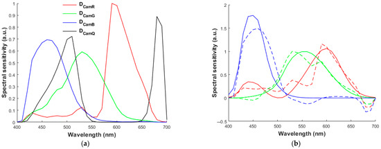
Figure 9b shows that the mean ERef is the smallest when λISGF = 590 nm and γ is small. This figure shows four data points represented by blue “+” symbols for λISGF = 590 nm. Figure 12a shows the full wavelength separation ΔλFS, edge width ΔλE, and cost function versus the Lagrange multiplier γ. The cost function increases smoothly with γ, but there are only four solutions. The four solutions are shown in Table 3, where the γ values shown are just for reference in that using multiple γ values may result in the same solution. Figure 12a also shows the mean ΔE00, mean ERef, and weighted chromaticity to reflectance error ratio wCR, where wCR is the ratio of the second term to the first term of the cost function defined in Equation (8), i.e.,
wCR = γ ΔE00,μ/ERef,μ.
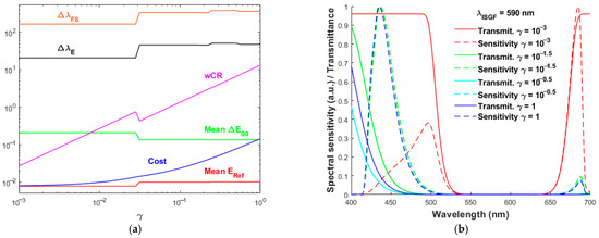
Figure 12.
(a) Mean RMS error ERef, mean color difference ΔE00, cost function, weighted error ratio wCR, filter full wavelength separation ΔλFS, and filter edge width ΔλE versus the Lagrange multipliers γ, where the quadcolor cameras are with the ISGF of wavelength λISGF = 590 nm. (b) The filter transmittance and spectral sensitivity for the cases of γ = 10−3, 10−1.5, 10−0.5, and 1 in (a).
From Figure 9b and Figure 12a, the wCR discontinuity at γ = 10−1.5 shows the transition from the smallest mean ERef to the second-smallest mean ERef when λISGF = 590 nm. Figure 12b shows the filter spectral transmittance and spectral sensitivity using λISGF = 590 nm and with γ = 10−3, 10−1.5, 10−0.5, and 1. The spectral transmittances of the latter three cases are apparently different, but their spectral sensitivities are nearly the same. Due to their small long-wavelength sensitivity lobes, their mean ERef and mean ΔE00 increase and decrease, respectively, compared with the case of γ = 10−3.
Table 2 shows the assessment metric statistics for three cases using the ISGF with λISGF = 600 nm and γ = 10−3, 10−1.65, and 1. The case of λISGF = 590 nm and γ = 10−3 is also shown. The statistics for the cases with smaller values of γ are similar. The best values in all cases shown in Table 2 are shown in bold red.
Compared with the case without a filter, using the ISGF of 590 nm in Table 2, the mean and PC98 of ERef decrease from 0.00928 and 0.0429 to 0.0078 and 0.02872, respectively; the percentage of test samples with a GFC > 0.99 (RFG99) increases from 98.311% to 99.156%; the mean and PC98 of ΔE00 decrease from 0.30618 and 1.53876 to 0.20859 and 0.8324, respectively. The improvements achieved by using the ISGF of 590 nm are significant.
Compared with the case without a filter, using the SGF of 400 nm in Table 2, the mean and PC98 of ΔE00 decrease to 0.1096 and 0.3748, respectively. Such reductions are significant, but the spectral reflectance error is larger.
Figure 7a–d also show the ERef, GFC, ΔE00, and SCI histograms for the cases of λISGF = 590 nm (γ = 10−3) and 600 nm (γ = 10−1.65). Since the mean values of ERef, ΔE00, and SCI are low for all cameras in Table 2, and the mean values of GFC are high, the counts in the low-value slots of ERef, ΔE00, and SCI and the counts in the high-value slot of GFC are very high. It can be seen from the enlarged sub-figures in Figure 7a,b that the counts in the worse slots using ISGF are apparently less than those using SGF and no filter (RGBF). From the enlarged sub-figures in Figure 7c,d, it can be seen that the counts in the worse slots without using the filter (RGBF) are larger than those using SGF and ISGF. The improvement in the four metrics using the ISGF is evident.
4.3. Recovered Spectrum Examples
Figure 13 shows the reconstructed spectra of the light reflected from the (a) 5Y 8.5/8, (b) 10P 7/8, (c) 2.5R 4/12, (d) 2.5G 7/6, (e) 10BG 4/8, and (f) 5PB 4/12 color chips, respectively, using the cameras considered in Figure 7, where the target spectra are also shown for comparison. The vertical axis of the figures is the spectral power density of the light reflected from the color chips before reaching the camera. The spectral reflectance recovered from the light reflected from the color chips in Figure 13a–f are shown in Figure 14a–f, respectively. These eight color chips were also taken as examples in [17,18], where the cases of (a) 5Y 8.5/8 and (b) 10P 7/8 color chips are interpolation examples and the other four are extrapolation examples. Regardless of using the II-LUT method or other methods in the literature, spectral recovery of extrapolation samples is challenging due to the lack of highly saturated training/reference samples. We can see that the recovered reflection spectra are accurate except for the (c) 2.5R 4/12 and (f) 5PB 4/12 color chips using the SGF with λSGF = 480 nm. The camera signal from the channel using the SGF with λSGF = 480 nm cannot provide a clue of the spectral characteristic from 650 nm to 700 nm. Thus, using the ISGFs shown in the figures is more reliable for spectrum reconstruction.
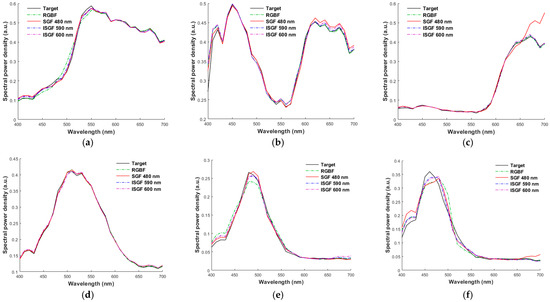
Figure 13.
Target and reconstructed reflection spectra using the quadcolor cameras considered in Figure 7. Munsell annotations of the color chips are (a) 5Y 8.5/8, (b) 10P 7/8, (c) 2.5R 4/12, (d) 2.5G 7/6, (e) 10BG 4/8, and (f) 5PB 4/12, respectively.
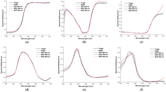
Figure 14.
(a–f) The target spectra and recovered reflectance spectra for the cases in Figure 13a–f, respectively.
Table 4 shows the color difference ΔE00 and RMS error ERef for the cases shown in Figure 13a–f and Figure 14a–f, respectively. For the worst case, recovering the (c) 2.5R 4/12 chip using the SGF with λSGF = 480 nm, the ERef value is poor, but the ΔE00 value is small. For this case, although the reconstructed reflection spectrum is poor, the spectrum with wavelengths between 650 nm and 700 nm contributes little to the tristimulus values.
5. Conclusions
The design of quadcolor cameras for spectral reflectance recovery was studied using the irradiance-independent look-up table method to reconstruct the reflection spectra from color samples. The RGB channels of the quadcolor camera were assumed to be the same as those of Nikon D5100. The 4th channel using a band-pass optical filter or notch optical filter was considered. The super-Gaussian function and the inverted super-Gaussian function were assumed to represent the spectral transmittance of the band-pass filter and the notch filter, respectively. The parameters of the filter were optimized to minimize the cost function consisting of the spectral reflectance error and the weighted color difference, where the weighting factor controls the contribution of the color difference.
The results of using the band-pass filters are summarized below.
- (1)
- The spectral sensitivity of the 4th channel with a peak wavelength between 500 nm and 550 nm reduces color difference owing to the improved fit of the camera spectral sensitivities to CMFs. Compared with the case without a filter, the mean color difference ΔE00 can be reduced from 0.3062 to 0.1096 when a filter was used, but the mean spectral reflectance error ERef increases from 0.00928 to 0.01047.
- (2)
- The spectral sensitivity of the 4th channel with a peak wavelength of around 685 nm reduces the spectral reflectance error because the sensitivities of RGB channels are small in this wavelength region, but it impairs the CMF fit. Compared with the case without a filter, the mean ERef and mean ΔE00 can be reduced to 0.00867 and 0.3012, respectively, when a filter was used.
When using the notch filter, the spectral sensitivity of the 4th channel can have two lobes with peak wavelengths at about 500 nm and 685 nm. Compared with the case without a filter, the mean ERef and mean ΔE00 can be reduced to 0.0078 and 0.2085, respectively, after using the optimized notch filter centered at 590 nm. The reduced spectral reflectance error is smaller than that obtained using the band-pass filter optimized for minimum ERef. Therefore, both spectral reflectance error and color difference can be effectively reduced.
Compared with D5100, where the mean ERef and mean ΔE00 are 0.01785 and 0.4778, respectively, using the quadcolor camera with the optimized notch filter can result in both mean metrics being 56.3% lower. Similarly, compared with the RGBF camera, using the quadcolor camera with the optimized notch filter can reduce the mean ERef and mean ΔE00 by 15.9% and 31.9%, respectively.
Since the RGB channels were not changed in this study, the optimized filters shown are for the Nikon D5100 camera. However, the spectral sensitivity design of a tricolor camera is usually as close to the CMFs as possible for color calibration, and its RGB signals cannot provide an effective clue of the spectral characteristics of a reflection spectrum in the long-wavelength region (650 nm to 700 nm) for spectrum reconstruction. Therefore, the technique of utilizing notch filters to improve the accuracy of spectral reflectance and chromaticity estimation can be applied to other quadcolor cameras modified from commercially available tricolor cameras.
Based on the above results, the design guidelines for the filters of a quadcolor camera are summarized as follows: Chromaticity accuracy can be increased by improving the fit of the camera spectral sensitivities to the CMFs. Spectral reflectance accuracy can be increased by adding a spectral sensitivity lobe in the long-wavelength region, where the CMF values are lower, but at the expense of reduced chromaticity accuracy. The optimal design is a trade-off between reflectance accuracy and chromaticity accuracy, depending on specific application requirements.
Author Contributions
Conceptualization, S.W. and Y.-C.W.; data collection, Y.-C.W.; methodology, Y.-C.W. and S.W.; software, Y.-C.W.; data analysis, Y.-C.W.; supervision, S.W.; writing—original draft, Y.-C.W.; writing—review and editing, S.W. All authors have read and agreed to the published version of the manuscript.
Funding
This research received no external funding.
Data Availability Statement
1. Spectral sensitivities of the Nikon D5100 camera are available: http://spectralestimation.wordpress.com/data/ (accessed on 10 July 2025). 2. Spectral reflectance of matt Munsell color chips are available: https://sites.uef.fi/spectral/munsell-colors-matt-spectrofotometer-measured/ (accessed on 10 July 2025).
Conflicts of Interest
The authors declare no conflicts of interest.
References
- Picollo, M.; Cucci, C.; Casini, A.; Stefani, L. Hyper-spectral imaging technique in the cultural heritage field: New possible scenarios. Sensors 2020, 20, 2843. [Google Scholar] [CrossRef]
- Candeo, A.; Ardini1, B.; Ghirardello, M.; Valentini, G.; Clivet, L.; Maury, C.; Calligaro, T.; Manzoni, C.; Comelli, D. Performances of a portable Fourier transform hyperspectral imaging camera for rapid investigation of paintings. Eur. Phys. J. Plus 2022, 137, 409. [Google Scholar] [CrossRef]
- Lu, B.; Dao, P.D.; Liu, J.; He, Y.; Shang, J. Recent advances of hyperspectral imaging technology and applications in agriculture. Remote Sens. 2020, 12, 2659. [Google Scholar] [CrossRef]
- Ahmed, M.T.; Monjur, O.; Khaliduzzaman, A.; Kamruzzaman, M. A comprehensive review of deep learning-based hyperspectral image reconstruction for agrifood quality appraisal. Artif. Intell. Rev. 2025, 58, 96. [Google Scholar]
- Vilela, E.F.; Ferreira, W.P.M.; Castro, G.D.M.; Faria, A.L.R.; Leite, D.H.; Lima, I.A.; Matos, C.S.M.; Silva, R.A.; Venzon, M. New Spectral Index and Machine Learning Models for Detecting Coffee Leaf Miner Infestation Using Sentinel-2 Multispectral Imagery. Agriculture 2023, 13, 388. [Google Scholar] [CrossRef]
- Ma, C.; Yu, M.; Chen, F.; Lin, H. An efficient and portable LED multispectral imaging system and its application to human tongue detection. Appl. Sci. 2022, 12, 3552. [Google Scholar] [CrossRef]
- Czempiel, T.; Roddan, A.; Leiloglou, M.; Hu, Z.; O’Neill, K.; Anichini, G.; Stoyanov, D.; Elson, D. RGB to hyperspectral: Spectral reconstruction for enhanced surgical imaging. Healthc. Technol. Lett. 2024, 11, 307–317. [Google Scholar] [CrossRef]
- Zhang, J.; Yao, P.; Wu, H.; Xin, J.H. Automatic color pattern recognition of multispectral printed fabric images. J. Intell. Manuf. 2022, 34, 2747–2763. [Google Scholar] [CrossRef]
- Kior, A.; Yudina, L.; Zolin, Y.; Sukhov, V.; Sukhova, E. RGB Imaging as a Tool for Remote Sensing of Characteristics of Terrestrial Plants: A Review. Plants 2024, 13, 1262. [Google Scholar] [CrossRef]
- Li, S.; Xiao, K.; Li, P. Spectra Reconstruction for Human Facial Color from RGB Images via Clusters in 3D Uniform CIELab* and Its Subordinate Color Space. Sensors 2023, 23, 810. [Google Scholar] [CrossRef]
- Valero, E.M.; Nieves, J.L.; Nascimento, S.M.C.; Amano, K.; Foster, D.H. Recovering spectral data from natural scenes with an RGB digital camera and colored Filters. Col. Res. Appl. 2007, 32, 352–360. [Google Scholar] [CrossRef]
- Tominaga, S.; Nishi, S.; Ohtera, R.; Sakai, H. Improved method for spectral reflectance estimation and application to mobile phone cameras. J. Opt. Soc. Am. A 2022, 39, 494–508. [Google Scholar] [CrossRef]
- Liang, J.; Wan, X. Optimized method for spectral reflectance reconstruction from camera responses. Opt. Express 2017, 25, 28273–28287. [Google Scholar] [CrossRef]
- He, Q.; Wang, R. Hyperspectral imaging enabled by an unmodified smartphone for analyzing skin morphological features and monitoring hemodynamics. Biomed. Opt. Express 2020, 11, 895–909. [Google Scholar] [CrossRef] [PubMed]
- Schaepman, M.E. Imaging spectrometers. In The SAGE Handbook of Remote Sensing; Warner, T.A., Nellis, M.D., Foody, G.M., Eds.; Sage Publications: Los Angeles, CA, USA, 2009; pp. 166–178. [Google Scholar]
- Cai, F.; Lu, W.; Shi, W.; He, S. A mobile device-based imaging spectrometer for environmental monitoring by attaching a lightweight small module to a commercial digital camera. Sci. Rep. 2017, 7, 15602. [Google Scholar] [CrossRef] [PubMed]
- Wen, Y.-C.; Wen, S.; Hsu, L.; Chi, S. Spectral reflectance recovery from the quadcolor camera signals using the interpolation and weighted principal component analysis methods. Sensors 2022, 22, 6228. [Google Scholar] [CrossRef] [PubMed]
- Wen, Y.-C.; Wen, S.; Hsu, L.; Chi, S. Irradiance independent spectrum reconstruction from camera signals using the interpolation method. Sensors 2022, 22, 8498. [Google Scholar] [CrossRef]
- Tzeng, D.Y.; Berns, R.S. A review of principal component analysis and its applications to color technology. Col. Res. Appl. 2005, 30, 84–98. [Google Scholar] [CrossRef]
- Agahian, F.; Amirshahi, S.A.; Amirshahi, S.H. Reconstruction of reflectance spectra using weighted principal component analysis. Col. Res. Appl. 2008, 33, 360–371. [Google Scholar] [CrossRef]
- Hamza, A.B.; Brady, D.J. Reconstruction of reflectance spectra using robust nonnegative matrix factorization. IEEE. Trans. Signal Process 2006, 54, 3637–3642. [Google Scholar] [CrossRef]
- Amirshahi, S.H.; Amirhahi, S.A. Adaptive non-negative bases for reconstruction of spectral data from colorimetric information. Opt. Rev. 2010, 17, 562–569. [Google Scholar] [CrossRef]
- Yoo, J.H.; Kim, D.C.; Ha, H.G.; Ha, Y.H. Adaptive spectral reflectance reconstruction method based on Wiener estimation using a similar training set. J. Imaging Sci. Technol. 2016, 60, 205031. [Google Scholar] [CrossRef]
- Nahavandi, A.M. Noise segmentation for improving performance of Wiener filter method in spectral reflectance estimation. Color Res. Appl. 2018, 43, 341–348. [Google Scholar] [CrossRef]
- Heikkinen, V.; Camara, C.; Hirvonen, T.; Penttinen, N. Spectral imaging using consumer-level devices and kernel-based regression. J. Opt. Soc. Am. A 2016, 33, 1095–1110. [Google Scholar] [CrossRef] [PubMed]
- Heikkinen, V. Spectral reflectance estimation using Gaussian processes and combination kernels. IEEE. Trans. Image Process 2018, 27, 3358–3373. [Google Scholar] [CrossRef]
- Wang, L.; Wan, X.; Xia, G.; Liang, J. Sequential adaptive estimation for spectral reflectance based on camera responses. Opt. Express 2020, 28, 25830–25842. [Google Scholar] [CrossRef]
- Lin, Y.-T.; Finlayson, G.D. On the Optimization of Regression-Based Spectral Reconstruction. Sensors 2021, 21, 5586. [Google Scholar] [CrossRef]
- Liu, Z.; Xiao, K.; Pointer, M.R.; Liu, Q.; Li, C.; He, R.; Xie, X. Spectral reconstruction using an iteratively reweighted regulated model from two illumination camera responses. Sensors 2021, 21, 7911. [Google Scholar] [CrossRef]
- Zhang, J.; Su, R.; Fu, Q.; Ren, W.; Heide, F.; Nie, Y. A survey on computational spectral reconstruction methods from RGB to hyperspectral imaging. Sci. Rep. 2022, 12, 11905. [Google Scholar] [CrossRef]
- Yao, P.; Wu, H.; Xin, J.H. Improving generalizability of spectral reflectance reconstruction using L1-norm penalization. Sensors 2023, 23, 689. [Google Scholar] [CrossRef]
- Huo, D.; Wang, J.; Qian, Y.; Yang, Y.-H. Learning to recover spectral reflectance from RGB images. IEEE Trans. Image Process 2024, 33, 3174–3186. [Google Scholar] [CrossRef]
- Abed, F.M.; Amirshahi, S.H.; Abed, M.R.M. Reconstruction of reflectance data using an interpolation technique. J. Opt. Soc. Am. A 2009, 26, 613–624. [Google Scholar] [CrossRef]
- Kim, B.G.; Han, J.; Park, S. Spectral reflectivity recovery from the tristimulus values using a hybrid method. J. Opt. Soc. Am. A 2012, 29, 2612–2621. [Google Scholar] [CrossRef]
- Kim, B.G.; Werner, J.S.; Siminovitch, M.; Papamichael, K.; Han, J.; Park, S. Spectral reflectivity recovery from tristimulus values using 3D extrapolation with 3D interpolation. J. Opt. Soc. Korea 2014, 18, 507–516. [Google Scholar] [CrossRef][Green Version]
- Chou, T.-R.; Hsieh, C.-H.; Chen, E. Recovering spectral reflectance based on natural neighbor interpolation with model-based metameric spectra of extreme points. Col. Res. Appl. 2019, 44, 508–525. [Google Scholar] [CrossRef]
- Wen, Y.-C.; Wen, S.; Hsu, L.; Chi, S. Auxiliary Reference Samples for Extrapolating Spectral Reflectance from Camera RGB Signals. Sensors 2022, 22, 4923. [Google Scholar] [CrossRef] [PubMed]
- Darrodi, M.M.; Finlayson, G.; Goodman, T.; Mackiewicz, M. Reference data set for camera spectral sensitivity estimation. J. Opt. Soc. Am. A 2015, 32, 381–391. [Google Scholar] [CrossRef]
- Kohonen, O.; Parkkinen, J.; Jaaskelainen, T. Databases for spectral color science. Col. Res. Appl. 2006, 31, 381–390. [Google Scholar] [CrossRef]
- Viggiano, J.A.S. A perception-referenced method for comparison of radiance ratio spectra and its application as an index of metamerism. Proc. SPIE 2002, 4421, 701–704. [Google Scholar]
- Mansouri1, A.; Sliwa1, T.; Hardeberg, J.Y.; Voisin, Y. An adaptive-PCA algorithm for reflectance estimation from color images. In Proceedings of the 19th International Conference on Pattern Recognition, Tampa, FL, USA, 8–11 December 2008. [Google Scholar]
Disclaimer/Publisher’s Note: The statements, opinions and data contained in all publications are solely those of the individual author(s) and contributor(s) and not of MDPI and/or the editor(s). MDPI and/or the editor(s) disclaim responsibility for any injury to people or property resulting from any ideas, methods, instructions or products referred to in the content. |
© 2025 by the authors. Licensee MDPI, Basel, Switzerland. This article is an open access article distributed under the terms and conditions of the Creative Commons Attribution (CC BY) license (https://creativecommons.org/licenses/by/4.0/).