Experimental Observation of Laser Planar Trapping

Abstract

This study experimentally demonstrates transverse symmetry breaking—a mechanism governing laser planar trapping—and distinguishes its unique role from related phenomena such as the lateral Goos–Hänchen shift and angular deviations. While the latter effects describe positional or angular beam displacements at interfaces, transverse symmetry breaking fundamentally alters the beam’s spatial symmetry, enabling unprecedented control over its intensity and phase profiles. Empirical results exhibit exceptional agreement with a recently proposed theoretical model, validating its predictive capability. Crucially, our findings highlight transverse symmetry breaking as a critical tool for tailoring beam profiles, advancing applications in optical trapping, structured light systems, and photonic device engineering, where symmetry manipulation unlocks new degrees of freedom in light–matter interactions.

1. Introduction

In recent years, there has been a growing interest in the scientific community regarding the analysis of optical beams transmitted through and reflected by dielectric blocks. This interest stems from the study of phenomena where the optical path deviates from the laws of geometric optics [1]. Two phenomena, namely the lateral displacement, also known as the Goos–Hänchen shift [2,3] and the angular deviation [4,5], have garnered particular attention [6,7,8,9].

Precise control over light beam shaping plays a pivotal role in advancing diverse technological domains. In optical communications, it enables optimized signal transmission efficiency and data integrity, forming the backbone of high-performance networks [10,11,12]. Within quantum optics, high-fidelity beam manipulation, including tailored spatial profiles, sub-wavelength alignment precision, and dynamic focal adjustments, is indispensable for robust quantum state preparation, manipulation, and measurement [13]. Emerging methodologies further underscore the versatility of this capability: Topological beam shaping, leveraging Jackiw–Rebbi states in metasurfaces, achieves unprecedented control over beam profiles [14]. High-energy laser systems utilize spatial light modulators (SLMs) to dynamically sculpt beam geometries for power delivery and thermal management [15,16,17]. Near-ideal hollow beams, critical for ultracold atom trapping and quantum simulation, exemplify precision in intensity and phase engineering [18]. These applications highlight the transformative potential of advanced beam shaping techniques across both fundamental research and industrial technologies.

Lateral displacements, parallel to the direction of the beam in the plane of incidence, manifest when an optical beam, propagating in a medium with a refractive index of n, encounters an interface with a second medium having a refractive index lower than n. These displacements, resulting from the interference between the incident and reflected waves, can be theoretically explained by the presence of a complex phase in the Fresnel coefficients [19]. Lateral displacements are typically small shifts proportional to the wavelength $\lambda$ of the optical beam, and they are amplified by a factor of $\sqrt{{\mathrm{w}}_0/\lambda }$, where ${\mathrm{w}}_0$ represents the beam waist, for incidences near the critical angle [1].

On the other hand, angular deviations refer to changes in the direction of the reflected and/or transmitted beam relative to the direction predicted by the laws of geometric optics. These deviations are theoretically explained by the asymmetry in the angular distribution of the optical beam caused by the magnitude of the Fresnel coefficients. The magnitude of these deviations is proportional to the axial distance and is amplified for incidences near the Brewster angle [1].

The upper transmission through a dielectric prism, as depicted in Figure 1, exhibits the combined effect of lateral displacement and angular deviation for incidences greater than the critical angle. This combination arises from the complex phase in the Fresnel coefficient of total internal reflection at the lower interface and the transmission coefficients through the left and right interfaces. A recent theoretical study showed cases where lateral displacements and angular deviations can offset each other [20].

The breaking of symmetry in the transverse components of a laser beam presents an intriguing phenomenon which bears similarities to the behavior observed in quantum mechanics when an electron beam traverses regions with varying potentials. The connection between quantum mechanics and optics motivated the exploration of transverse symmetry breaking in the context of lower transmission through a dielectric prism. This transverse symmetry breaking, resembling a lensing effect on the beam waist within the plane of incidence, gives rise to the intriguing phenomenon of laser planar trapping. A recent article has presented an analytical formula to describe this phenomenon [21].

Lateral shift, angular deviations, and transverse symmetry breaking represent three distinct optical phenomena. The first occurs when Fresnel coefficients become complex as a beam traverses or is reflected at the interface between two media where the refractive index of the first medium exceeds that of the second. This introduces an additional optical phase accumulation. The second phenomenon, which can also arise with real Fresnel coefficients, stems from their influence on the Gaussian intensity distribution of the beam. Finally, the third phenomenon, the primary focus of our study, originates from the presence of additional spatial phase terms in scenarios where the angles of incidence and emergence at the prism interface differ, as observed in the lower-transmission regime of an optical prism.

In the following section, we provide a concise overview of the theoretical model of transverse symmetry breaking using the angular formalism for the convenience of the reader. Subsequently, we delve into the experimental setup and analysis pertaining to this phenomenon. Finally, in the last section, we present our conclusions, explore potential applications, and outline directions for future investigations.

2. Materials and Methods

Let us examine the propagation of a Gaussian optical beam as it travels from its source to a dielectric prism. The electric field of the incident beam can be mathematically described using the following integral expression:

$$E=E_0\int d\theta d\alpha G(\theta ,\alpha )exp\left[i\mathsf{\Psi }(\theta ,\alpha )\right],$$

(1)

where

$$G(\theta ,\alpha )={\displaystyle \frac{z_{\mathrm{R}}}{\lambda }}exp\left\{-{\left({\displaystyle \frac{z_{\mathrm{R}}}{{\mathrm{w}}_0}}\right)}^2\left[{\left(\theta -{\theta }_0\right)}^2+{\alpha }^2\right]\right\}$$

represents the angular distribution centered at $({\theta }_0,0)$, ${\theta }_0$ is the angle formed by the incident beam with the normal to the first interface in the incidence plane, $\lambda$ denotes the wavelength of the optical beam, ${\mathrm{w}}_0$ is the beam waist, and $z_{\mathrm{R}}=\pi {\mathrm{w}}_0^2/\lambda$ represents the Rayleigh axial range. The optical spatial phase is given by

$$\mathsf{\Psi }(\theta ,\alpha )=k(x_{1}sin\theta +z_{1}cos\theta )cos\alpha +ysin\alpha ,$$

where $\theta$ is the angular integration parameter in the incidence plane, $\alpha$ is the angular integration parameter in the plane perpendicular to the incidence plane, and $(x_1,z_1)$ refers to the coordinate system of the first interface, as shown in Figure 1.

Recognizing that the exponential term in the angular distribution contains the factor $z_R/{\mathrm{w}}_0\propto {\mathrm{w}}_0/\lambda \gg 1$, we can conclude that the angular distribution at $({\theta }_0,0)$ is highly peaked. Therefore, we can expand the spatial optical phase $\mathsf{\Psi }(\theta ,\alpha )$ in a Taylor series up to the second order around $({\theta }_0,0)$,

$$\begin{array}{ccc}\hfill \mathsf{\Psi }(\theta ,\alpha )& =& \mathsf{\Psi }({\theta }_0,0)+kz\hfill \\ & & +kx(\theta -{\theta }_0)+ky\alpha \hfill \\ & & -kz[{(\theta -{\theta }_0)}^2+{\alpha }^2]/2,\hfill \end{array}$$

where $(x,z)$ represents the coordinate system of the incident beam. By employing this expansion, we can perform an analytical integration of the right-hand side of Equation (1). This integration results in obtaining the widely recognized closed formula for the incident beam

$$\begin{array}{ccc}\hfill I& =& {\left|{\displaystyle \frac{E_0{e}^{ikz}}{1+iz/z_{\mathrm{R}}}}exp\left[-{\displaystyle \frac{x^2+y^2}{{\mathrm{w}}_0^2(1+iz/z_{\mathrm{R}})}}\right]\right|}^2\hfill \\ & =& I_0{\left[{\displaystyle \frac{{\mathrm{w}}_0}{\mathrm{w}\left(z\right)}}\right]}^{2}exp\left[-2{\displaystyle \frac{x^2+y^2}{{\mathrm{w}}^2\left(z\right)}}\right],\hfill \end{array}$$

(2)

where $I_0={\left|E_0\right|}^2$ and $\mathrm{w}\left(z\right)={\mathrm{w}}_0\sqrt{1+{(z/z_{\mathrm{R}})}^2}$. Equation (2) highlights the well-known Gaussian symmetry exhibited by the transverse components of the incident beam.

Let us now analyze the integral form of the lower transmitted beam,

$$E_{*}^{\left[\sigma \right]}=E_0\int d\theta d\alpha T_{*}^{\left[\sigma \right]}\left(\theta \right)G(\theta ,\alpha )exp\left[i{\mathsf{\Psi }}_{*}(\theta ,\alpha )\right],$$

(3)

where

$$\begin{array}{ccc}\hfill T_{*}^{\left[\sigma \right]}\left(\theta \right)& =& {\left[{\displaystyle \frac{4{\mathrm{r}}_{\sigma }cos\theta cos\phi }{\left(cos\theta +{\mathrm{r}}_{\sigma }cos\psi \right)\left({\mathrm{r}}_{\sigma }cos\phi +cos\varphi \right)}}\right]}^2\hfill \\ & & exp[i(ncos\phi -cos\varphi )kd/\sqrt{2}],\hfill \\ & =& t_{*}^{\left[\sigma \right]}\left(\theta \right)exp\left[i\mathsf{\Phi }\left(\theta \right)\right],\hfill \end{array}$$

represents the Fresnel coefficient describing the transmission of electric and magnetic waves through the first and lower interfaces, $\{{\mathrm{r}}_{\mathrm{te}},{\mathrm{r}}_{\mathrm{tm}}\}=\{n,1/n\}$, and $\mathsf{\Phi }\left(\theta \right)$ is the phase accounting for the distance, d, between the incidence point and the point of transmission at the lower interface, where the continuity equations have been imposed.

The optical spatial phase of the lower transmitted beam, denoted as ${\mathsf{\Psi }}_{*}(\theta ,\alpha )$ in Equation (3), is expressed in terms of the lower transmitted angular integration parameters $(\varphi ,\alpha )$ and the coordinate system of the second interface $(x_2,z_2)$:

$${\mathsf{\Psi }}_{*}(\theta ,\alpha )=k(x_{2}sin\varphi +z_{2}cos\varphi )cos\alpha +ysin\alpha .$$

Similarly to the approach used for the incident beam, to obtain analytical expressions for the lower transmitted beam, we can expand the spatial optical phase around $({\theta }_0,0)$, obtaining

$$\begin{array}{ccc}\hfill {\mathsf{\Psi }}_{*}(\theta ,\alpha )& =& {\mathsf{\Psi }}_{*}({\theta }_0,0)+k{z}_{*}+k{x}_{*}{\varphi }_0^{\prime }(\theta -{\theta }_0)\hfill \\ & & +ky\alpha -k{z}_{*}[{\varphi }_0^{{\prime }^2}{(\theta -{\theta }_0)}^2+{\alpha }^2]/2\hfill \\ & & +k{x}_{*}{\varphi }_0^{\prime \prime }{(\theta -{\theta }_0)}^2/2.\hfill \end{array}$$

Given that the axial coordinate is significantly larger than the transverse coordinates, we can neglect the last term in the right-hand side of the previous equation. The expansion of the Fresnel phase is given by

$$\begin{array}{ccc}\hfill \mathsf{\Phi }\left(\theta \right)& =& {\mathsf{\Phi }}_0-k{d}_{*}{\varphi }_0^{\prime }(\theta -{\theta }_0),\hfill \end{array}$$

where ${\mathsf{\Phi }}_0$ represents the zero order phase,

$$d_{*}=(tan\phi cos\varphi -sin\varphi )d/\sqrt{2}$$

the displacement of the beam predicted by Snell’s law.

To realize the analytical integration of the right-hand side of Equation (3), it is necessary to expand the Fresnel coefficient as follows:

$$t_{*}^{\left[\sigma \right]}\left(\theta \right)=t_{*,0}^{\left[\sigma \right]}+{\left[t_{*}^{\left[\sigma \right]}\right]}_0^{\prime }(\theta -{\theta }_0)$$

After performing the necessary algebraic manipulations, we obtain

$$\begin{array}{ccc}\hfill I_{*}^{\left[\sigma \right]}& =& I_0{t}_{*,0}^{\left[\sigma \right]}\hfill \\ & & \left[1+{\left({\displaystyle \frac{{\left[t_{*}^{\left[\sigma \right]}\right]}_0^{\prime }(x_{*}-d_{*}){\varphi }_0^{\prime }+t_{*,0}^{\left[\sigma \right]}{z}_{*}{\varphi }_0^{{\prime }^2}}{t_0{z}_{\mathrm{R}}}}\right)}^2\right]\hfill \\ & & {\displaystyle \frac{{\mathrm{w}}_0}{\mathrm{w}\left(z_{*}{\varphi }_0^{{\prime }^2}\right)}}exp\left[-2{\displaystyle \frac{{(x_{*}-d_{*})}^2{\varphi }_0^{{\prime }^2}}{{\mathrm{w}}^2\left(z_{*}{\varphi }_0^{{\prime }^2}\right)}}\right]\hfill \\ & & {\displaystyle \frac{{\mathrm{w}}_0}{\mathrm{w}\left(z_{*}\right)}}exp\left[-2{\displaystyle \frac{y^2}{{\mathrm{w}}^2\left(z_{*}\right)}}\right].\hfill \end{array}$$

The quadratic term,

$${\left({\displaystyle \frac{{\left[t_{*}^{\left[\sigma \right]}\right]}_0^{\prime }(x_{*}-d_{*}){\varphi }_0^{\prime }+t_{*,0}^{\left[\sigma \right]}{z}_{*}{\varphi }_0^{{\prime }^2}}{t_0{z}_{\mathrm{R}}}}\right)}^2,$$

is responsible for the phenomenon of angular deviations in the lower transmitted beam. These deviations arise due to the breaking of the symmetry caused by the Fresnel coefficient, which acts as a modulating factor on the incident Gaussian angular distribution. However, for the purpose of this paper and our focus on transverse symmetry breaking, we can neglect the term related to angular deviations. By introducing

$${\mathrm{w}}_{*}\left(z_{*}\right)={\displaystyle \frac{{\mathrm{w}}_0}{{\varphi }_0^{\prime }}}\sqrt{1+{\left({\displaystyle \frac{z_{*}{\varphi }_0^{{\prime }^2}}{z_{\mathrm{R}}}}\right)}^2},$$

Equation (4) can be rewritten as

$$\begin{array}{ccc}\hfill I_{*}^{\left[\sigma \right]}& =& I_0{t}_{*,0}^{\left[\sigma \right]}{\displaystyle \frac{\mathrm{w}\left(0\right)}{\mathrm{w}\left(z_{*}\right)}}exp\left[-2{\displaystyle \frac{y^2}{{\mathrm{w}}^2\left(z_{*}\right)}}\right]\hfill \\ & & {\displaystyle \frac{{\mathrm{w}}_{*}\left(0\right)}{{\mathrm{w}}_{*}\left(z_{*}\right)}}exp\left[-2{\displaystyle \frac{{(x_{*}-d_{*})}^2}{{\mathrm{w}}_{*}^2\left(z_{*}\right)}}\right].\hfill \end{array}$$

(4)

This simplified expression for the lower transmitted intensity clearly demonstrates the transverse breaking of symmetry between the $x_{*}$ and $y_{*}$ coordinates. The dielectric prism serves as a lensing tool, altering the beam waist of the transverse plane parallel to the incidence plane. The transverse breaking of symmetry can be characterized by the factor

$$\rho (n,{\theta }_0)={\displaystyle \frac{{\mathrm{w}}_{*}\left(0\right)}{\mathrm{w}\left(0\right)}}={\displaystyle \frac{1}{{\varphi }_0^{\prime }}}={\displaystyle \frac{cos{\psi }_{0}cos{\varphi }_0}{cos{\theta }_{0}cos{\phi }_0}}.$$

(5)

This factor has been the subject of our experimental investigation. It is important to note that $\rho$ is solely dependent on the incidence angle, ${\theta }_0$, and the refractive index of the dielectric prism, n. Unlike the breaking of symmetry in the angular distribution that causes angular deviations, $\rho$ is independent of the polarization of the optical beam. This highlights that the transverse breaking of symmetry is a polarization-independent phenomenon.

In nearly all the experimental scenarios, the relative error in the refractive index is significantly smaller than the relative error in the angle of incidence. Consequently, after performing the requisite algebraic steps, the uncertainty in the $\rho$ formula is expressed as follows:

$$\mathsf{\Delta }\rho (n,{\theta }_0)=\rho \sqrt{{tan}^2\theta +{\displaystyle \frac{{cos}^2{\theta }_0({tan}^2{\psi }_0+{tan}^2{\phi }_0)}{n^2{cos}^2{\psi }_0}}+{\displaystyle \frac{{cos}^2{\theta }_0{cos}^2{\phi }_0{tan}^2{\varphi }_0}{{cos}^2{\psi }_0{cos}^2{\varphi }_0}}}\mathsf{\Delta }{\theta }_0.$$

Finally, we note that the universal formula in Equation (5) can be directly generalized to a prism with apex angle $\alpha$ by substituting ${\phi }_0={\psi }_0+\pi /4$ with ${\phi }_0={\psi }_0+\alpha$. The upper bound for the incidence angle is dictated by the geometric constraint ensuring that the beam transmitted through the first interface intersects the second interface, thereby enabling the lower transmission regime of the beam.

We conclude this section by noting that the transverse breaking of symmetry is not present in the upper transmitted beam because, due to the symmetry of the system, the upper transmission angle is equal to the incidence angle. This mimics a symmetric barrier in quantum mechanics, which does not produce any transverse symmetry breaking in the transmitted beam.

3. Results

Figure 1 depicts the geometric arrangement of the experimental setup. A Gaussian beam from a DPSS laser (wavelength $\lambda =532.0$ nm, power 1.5 mW) is shaped by a lens system into two distinct collimated configurations. In the first configuration, the beam passes through a lens with focal length $f=50$ cm, producing a focused beam with a minimum waist size of ${\mathrm{w}}_0=96.7\pm 1.2\mathsf{\mu }$m at the focal plane. This waist is positioned at the air–dielectric interface of a right-angle BK7 prism ($n=1.515$ at $\lambda =532$ nm). In the second configuration, the beam traverses a telescope system (lens focal lengths $f=10$ cm and $f=5$ cm), generating a collimated beam with a waist radius ${\mathrm{w}}_0=498.6\pm 10.2\mathsf{\mu }$m. Unlike the focused case, the collimated configuration does not require precise prism placement.

The BK7 prism is mounted on a high-precision rotation stage with a vernier scale, enabling adjustment of the angle of incidence ($\theta$) with a resolution of $0.3°$. For alignment consistency, the prism front leg coincides with the rotation axis of the mount.

After transmission through the prism, the knife-edge method is applied to the lower transmitted beam to analyze its spatial profile within the plane of incidence. Measurements are performed at varying $\theta$ and longitudinal positions (z-axis) by incrementally advancing the knife edge across the beam. The transmitted power is recorded as the edge obstructs 10 – $90\%$ of the total beam power, enabling precise reconstruction of the beam spatial characteristics for each configuration.

To specifically investigate the symmetry-breaking effect, we narrow our focus to the analysis of the lower transmitted beam in the case of both focused and collimated beams. After passing through the front leg of the prism, the beam interacts with the lower dielectric interface, and its transmitted portion is intercepted by a razor blade. This setup enables us to perform power measurements necessary for the knife-edge method. The lower beam propagates at an angle of ${\gamma }_0$ with respect to the normal to the lower interface, as illustrated in Figure 1.

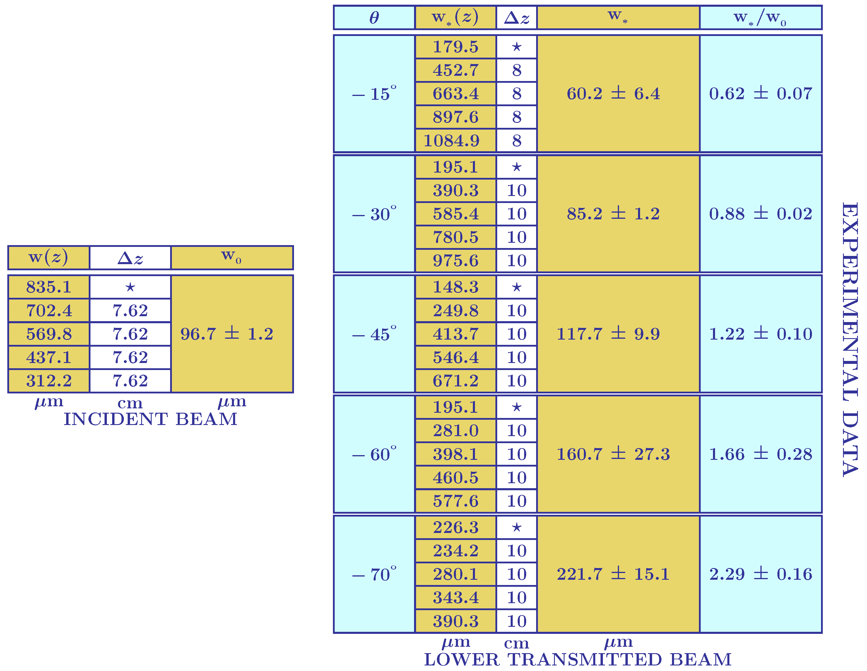
In the first configuration, we employ the knife-edge method to characterize the beam width $\mathrm{w}\left(z\right)$ as a function of propagation distance z along the free incoming beam. The data obtained from the knife-edge method, presented on the left side of Figure 2, allow us to determine not only the minimum beam waist, ${\mathrm{w}}_0=96.7\pm 1.2\mathsf{\mu }$m, but also its corresponding position. Subsequently, we position the front leg of the prism precisely at the minimum beam waist position to perform the knife-edge method on the lower transmitted beam. We carry out this method for various angles of incidence. For each angle, the knife-edge method measures the beam profile at different z values, capturing the power ranging from $10\%$ to $90\%$. The results obtained, shown on the right side of Figure 2, include the beam profile ${\mathrm{w}}_{*}\left(z\right)$ as well as the new minimum beam waist ${\mathrm{w}}_{*}$. 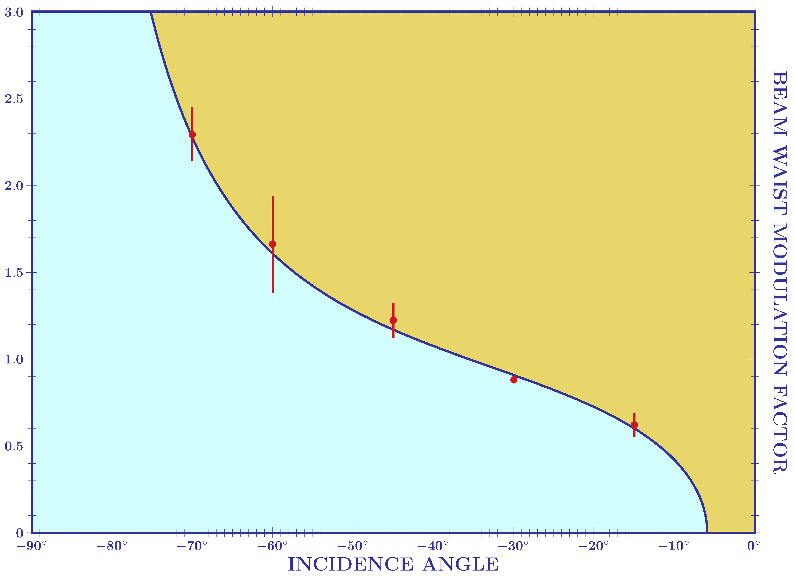The experimental values for the ratio ${\mathrm{w}}_{*}/{\mathrm{w}}_0$ are listed in the last column of Figure 2 and are utilized in the plot presented in Figure 3.

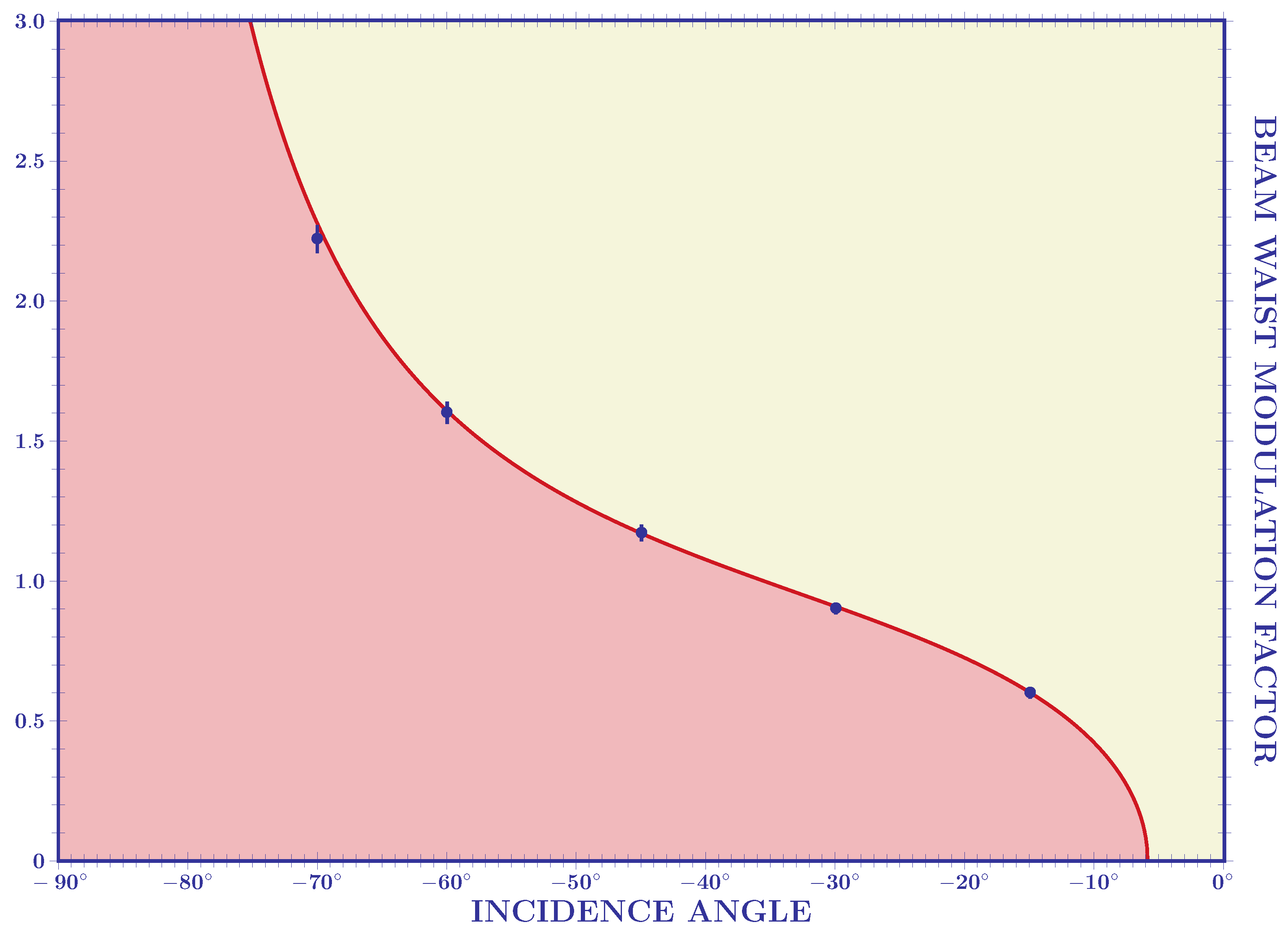
In the second configuration, we utilize the knife-edge method along the free incoming beam to verify the value of ${\mathrm{w}}_0$ as the beam is collimated. The knife-edge method data, presented on the left side of Figure 4, provide the beam radius, i.e., ${\mathrm{w}}_0=498.6\pm 10.2\mathsf{\mu }$m. For each angle of incidence, the knife-edge method measures the lower output power at various z values, covering the range from $10\%$ to $90\%$, to obtain the beam profile ${\mathrm{w}}_{*}$. The right side of Figure 4 displays, for each angle of incidence, the new minimum beam waist determined by taking the mean value and standard deviation from five measurements. Additionally, the experimental values for the ratio ${\mathrm{w}}_{*}/{\mathrm{w}}_0$ are listed in the last column of Figure 4 and are employed in the plot presented in Figure 5.

The plots given in Figure 3 and Figure 5 compare the experimental data with the theoretical curves (represented by blue solid lines) obtained using Equation (2). The remarkable agreement between the experimental data and theoretical results confirms the validity of the theoretical predictions [21].

4. Discussion

In the propagation of laser beams through dielectric prisms, studies usually concentrate on the detailed analysis of the upper transmitted beam. This is primarily because phenomena such as lateral beam displacements can only occur in the beam transmitted above, as a consequence of total internal reflection. Remarkably, due to the prism’s symmetry, this transmitted beam does not display any transverse asymmetry.

Recently, a theoretical study on laser planar trapping [21] has unveiled a transverse symmetry-breaking phenomenon in the lower transmitted beam. Additionally, it has proposed an analytical formula to characterize this intriguing effect. This formula, Equation (2), relies solely on two factors: the refractive index of the prism and the angle of incidence. The universality of $\rho (n,{\theta }_0)$ has been confirmed through the experimental analysis presented in this study, which involved two different experimental configurations. Notably, the experimental data have demonstrated a remarkable agreement with the theoretical formula; see Figure 3 and Figure 5. Once the theoretical formula is experimentally validated, it will prove valuable in utilizing the axial asymmetry caused by the prism as a novel means of controlling optical beam profiles.