
Correction of Error Interference Fringes Based on Automatic Spectral Analysis


Abstract
1. Introduction
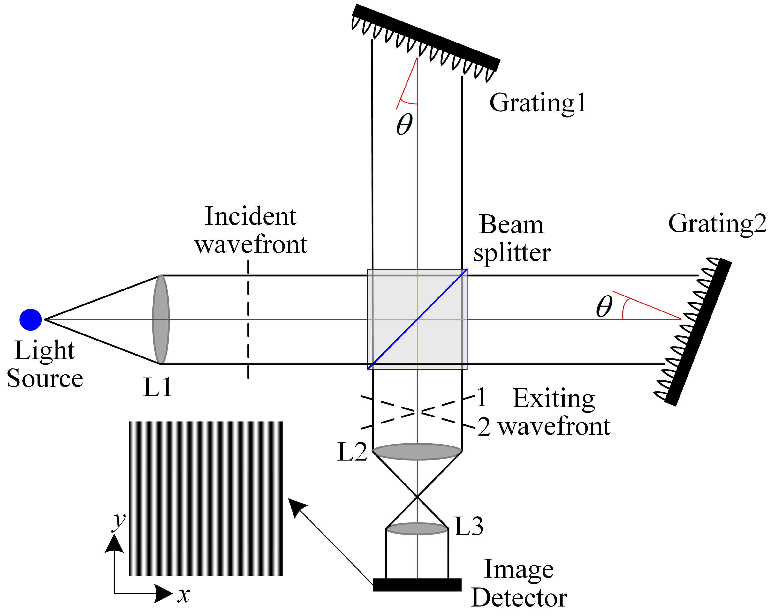
2. Method
3. Experiments
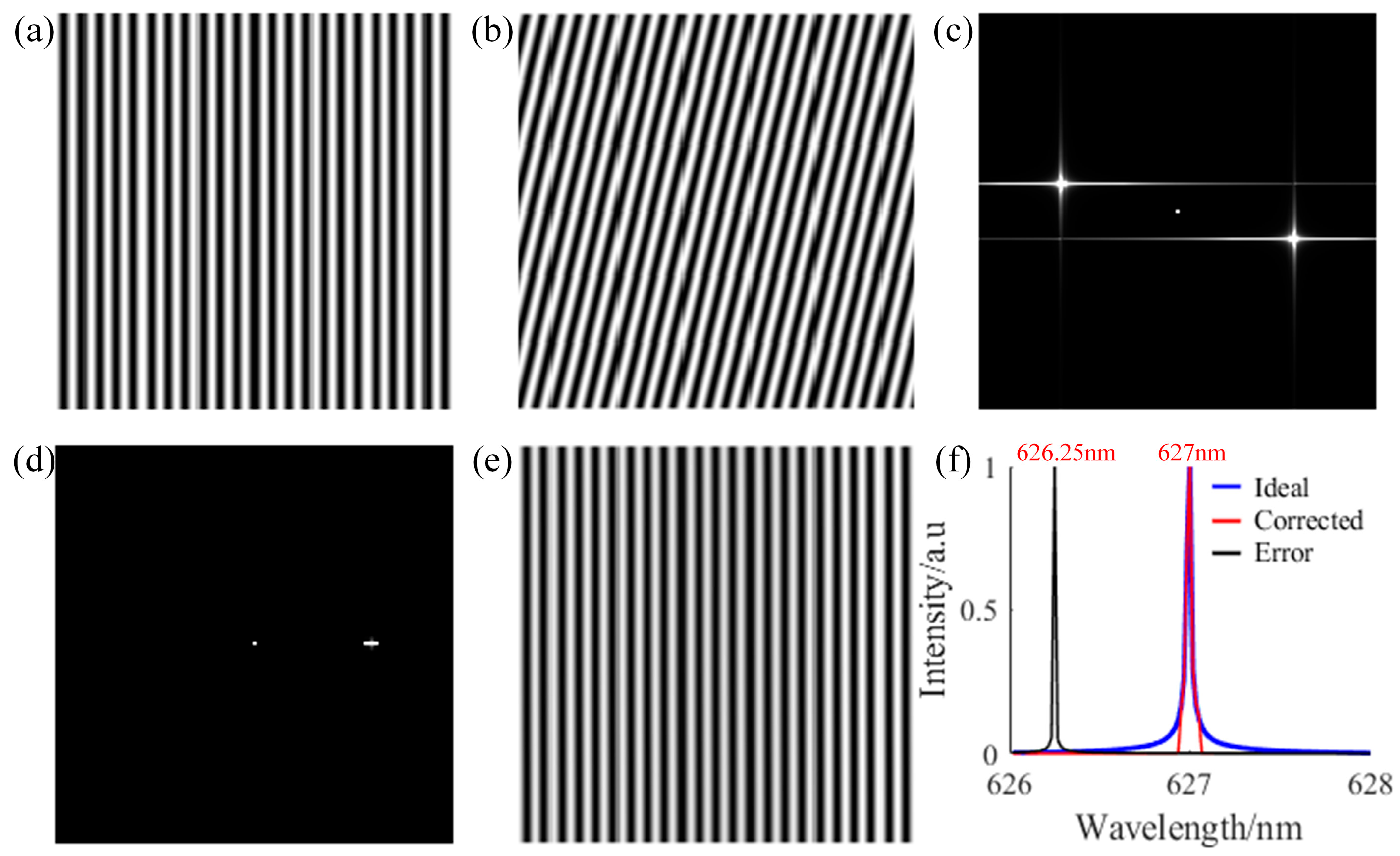
3.1. Simulation Analysis of Correction for Error Interferogram in Monochromatic Light
3.2. Simulation Analysis of Correction for Error Interferogram in Polychromatic Light
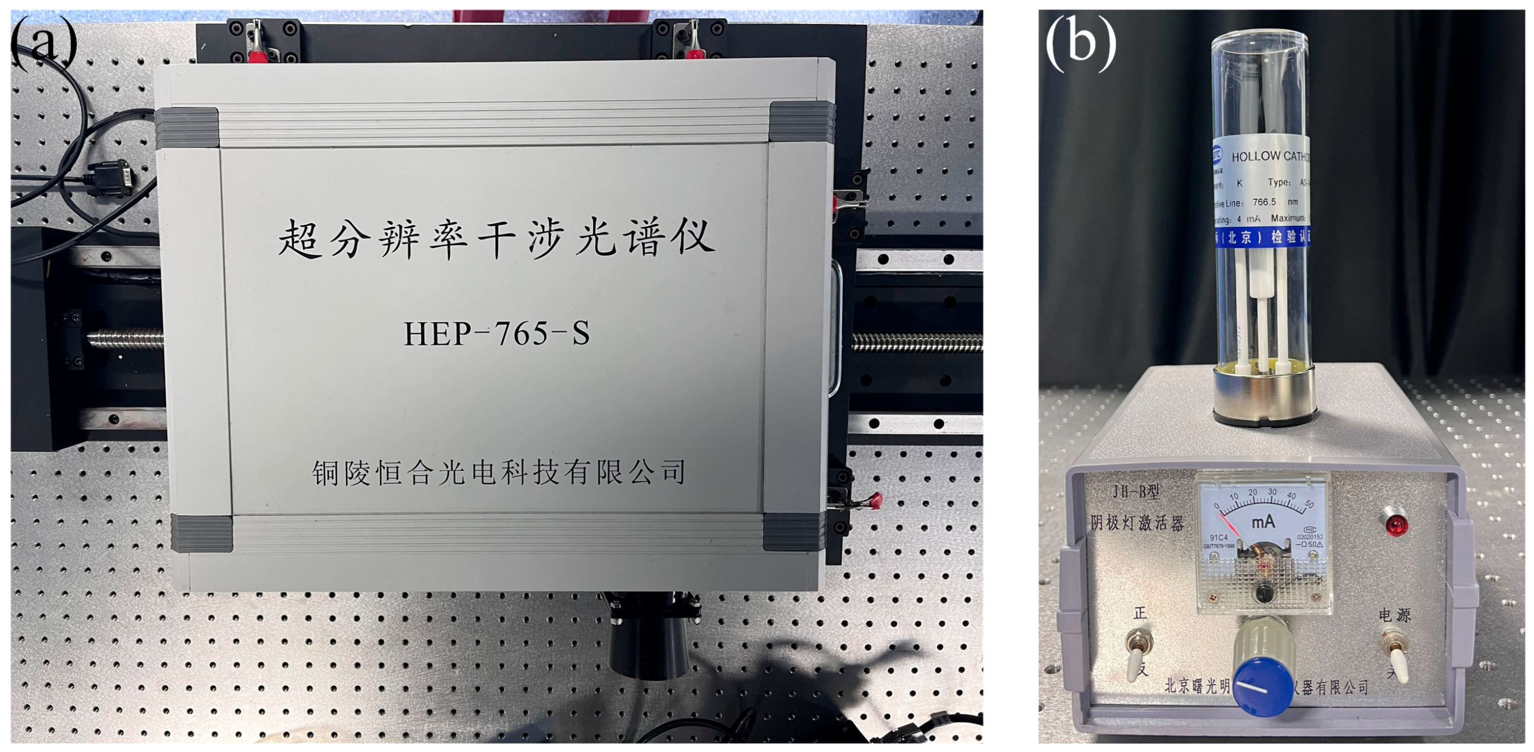
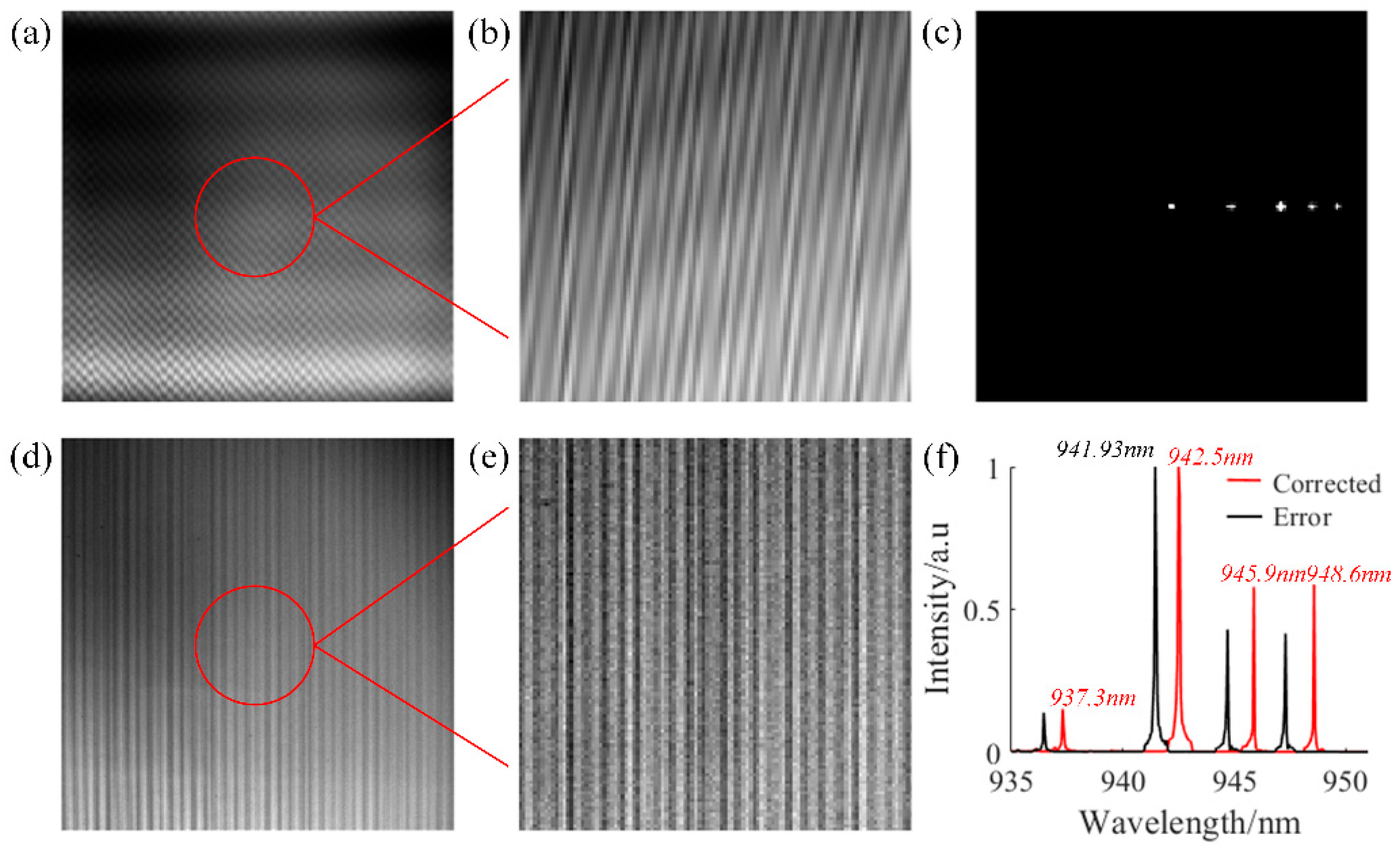
3.3. Correction of Potassium Lamp Interference Pattern
3.4. Correction Experiment of Neon Lamp Interference Pattern
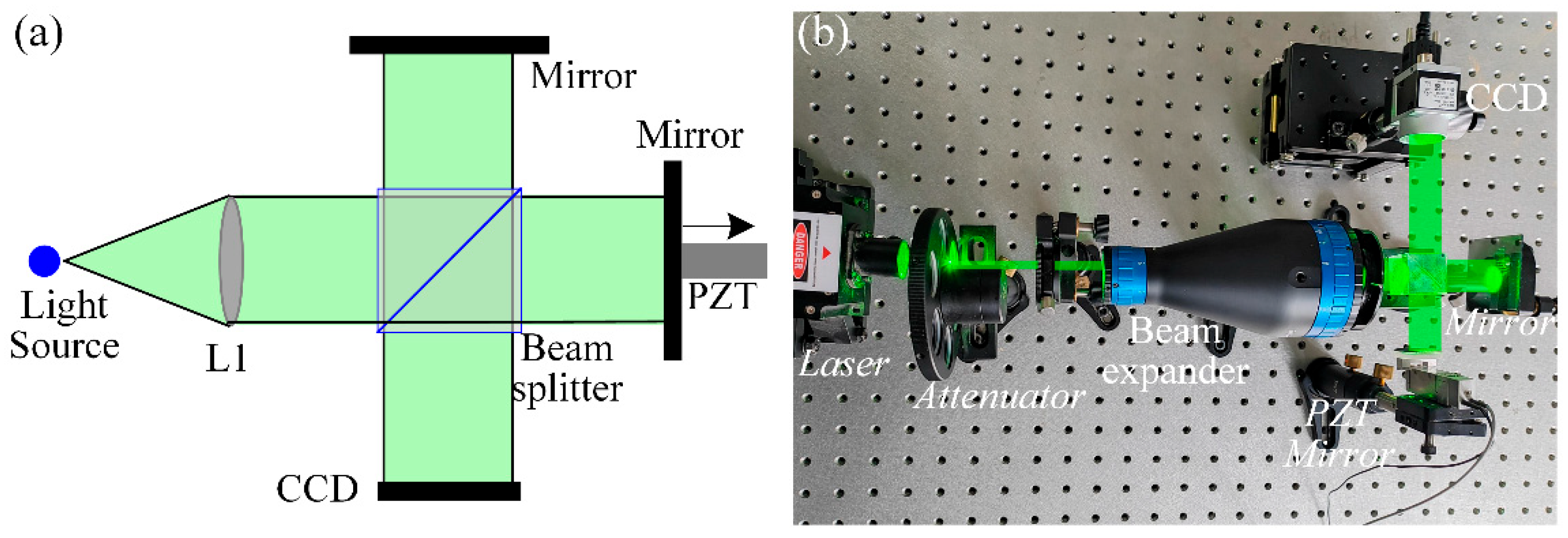
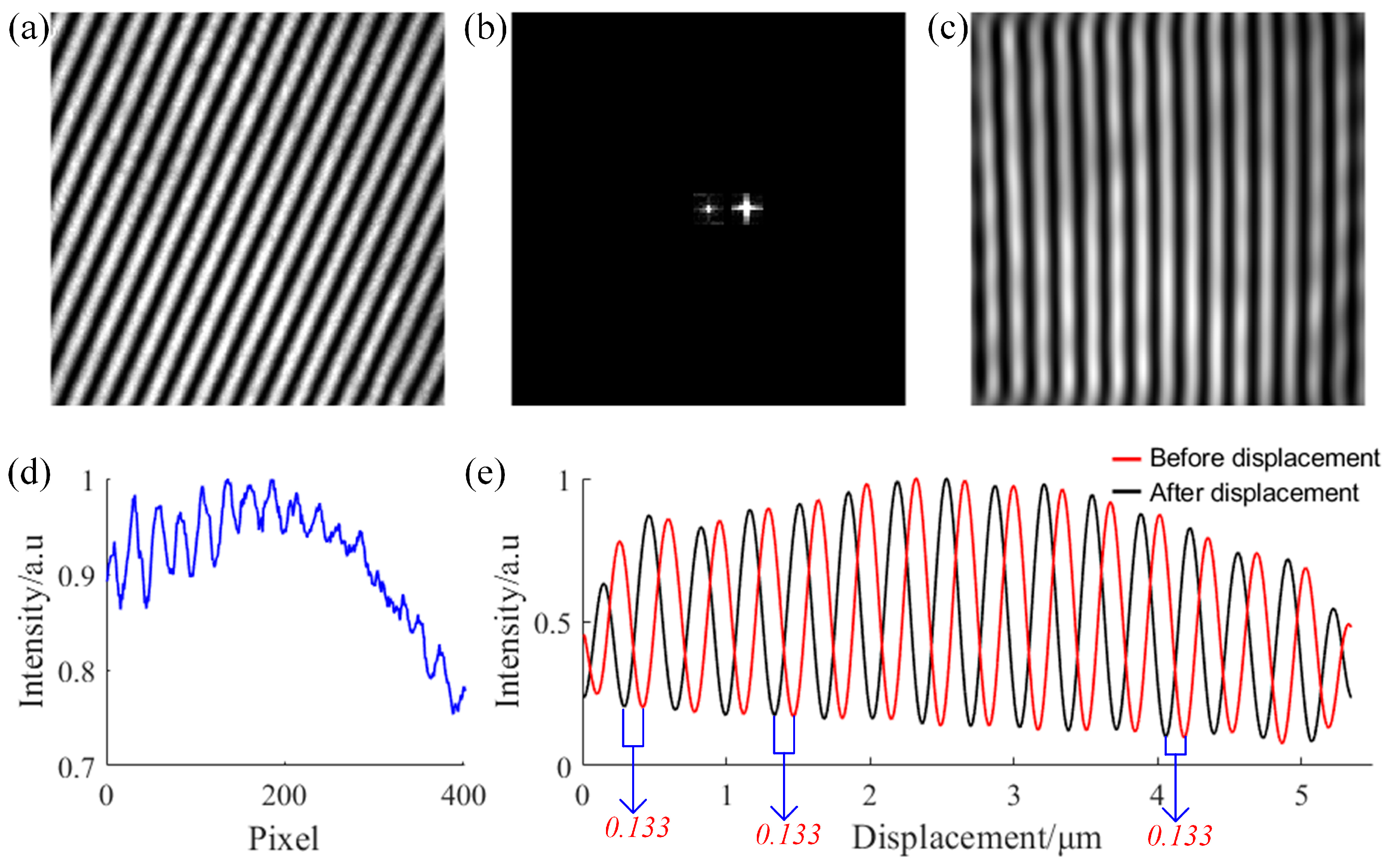
3.5. Application of Corrected Interference Patterns in Displacement Measurement
4. Discussion and Conclusions
Author Contributions
Funding
Data Availability Statement
Conflicts of Interest
References
- Wang, Q.; Luo, H.; Li, Z.; Ding, Y.; Xiong, W. Analysis of signal-to-noise ratio of spatial heterodyne spectroscopy. Measurement 2024, 237, 115180. [Google Scholar] [CrossRef]
- Wang, Q.; Luo, H.; Li, Z.; Shi, H.; Bai, Y.; Xiong, W. Digital micromirror device and spatial heterodyne spectroscopy combined modulation interference spectroscopy. Opt. Commun. 2022, 507, 127595. [Google Scholar] [CrossRef]
- Wang, Q.; Luo, H.; Bai, Y.; Ding, Y.; Li, Z.; Xiong, W. Optical system design of a DMD–SHS combined modulation interference spectrometer. Appl. Opt. 2023, 62, 2154–2160. [Google Scholar] [CrossRef] [PubMed]
- Long, X.; Huang, Z.; Tian, Y.; Du, J.; Liu, Y. High-resolution on-chip spatial heterodyne Fourier transform spectrometer based on artificial neural network and PCSBL reconstruction algorithm. Opt. Express 2023, 31, 33608–33621. [Google Scholar] [CrossRef]
- Zhang W-l Liu, Z.-Y.; Wang, H.; Chen, Y.; Wang, Y.; Zhao, Z.-Z.; Sun, T. Research status of spatial Heterodyne spectroscopy—A review. Microchem. J. 2021, 166, 106228. [Google Scholar] [CrossRef]
- Lenzner, M.; Diels, J.-C. Concerning the Spatial Heterodyne Spectrometer. Opt. Express 2016, 24, 1829–1839. [Google Scholar] [CrossRef] [PubMed]
- Englert, C.R.; Harlander, J.M.; Brown, C.M.; Marr, K.D. Spatial heterodyne spectroscopy at the Naval Research Laboratory. Appl. Opt. 2015, 54, F158–F163. [Google Scholar] [CrossRef]
- Hosseini, S. Characterization of cyclical spatial heterodyne spectrometers for astrophysical and planetary studies. Appl. Opt. 2019, 58, 2311–2319. [Google Scholar] [CrossRef]
- Zettner, A.; Gojani, A.B.; Schmid, T.; Gornushkin, I.B. Evaluation of a Spatial Heterodyne Spectrometer for Raman Spectroscopy of Minerals. Minerals 2020, 10, 202. [Google Scholar] [CrossRef]
- Hu, G.; Xiong, W.; Luo, H.; Shi, H.; Li, Z.; Shen, J.; Fang, X.; Xu, B.; Zhang, J. Raman Spectroscopic Detection for Simulants of Chemical Warfare Agents Using a Spatial Heterodyne Spectrometer. Appl. Spectrosc. 2017, 72, 151–158. [Google Scholar] [CrossRef]
- Qiu, J.; Qi, X.; Li, X.; Ma, Z.; Jirigalantu; Tang, Y.; Mi, X.; Zheng, X.; Zhang, R. Bayanheshig, Development of a spatial heterodyne Raman spectrometer with echelle-mirror structure. Opt. Express 2018, 26, 11994–12006. [Google Scholar] [CrossRef] [PubMed]
- Shi, H.; Xiong, W.; Luo, H.; Li, Z. Ground observation result of an OH radical hyper-resolution spectrometer for the middle and upper atmosphere. Appl. Opt. 2019, 58, 5602–5611. [Google Scholar] [CrossRef]
- Luo, H.; Wei, X.; Shi, H.; Chen, D.; Li, Z. Error analysis of field of view registration accuracy of hyper-resolution spatial heterodyne spectrometer for hydroxyl radical OH. Proc. SPIE 2019, 11337, 1133705. [Google Scholar]
- Bartula, R.J.; Ghandhi, J.B.; Sanders, S.T.; Mierkiewicz, E.J.; Roesler, F.L.; Harlander, J.M. OH absorption spectroscopy in a flame using spatial heterodyne spectroscopy. Appl. Opt. 2007, 46, 8635–8640. [Google Scholar] [CrossRef]
- Li, X.; Riedel, J.; You, Y. Practical high-resolution spectroscopy with a spatial heterodyne spectrometer: Determination of instrumental function for lineshape recovery. Spectrochim. Acta Part B At. Spectrosc. 2024, 221, 107053. [Google Scholar] [CrossRef]
- Kumar, V. Analysis of Atomic Structure Using Spectroscopy: An Emission and Absorption Line Spectrum Study. Int. Res. J. Adv. Sci. Hub. 2024, 6, 348–357. [Google Scholar] [CrossRef]
- Englert, C.R.; Harlander, J.M.; Cardon, J.G.; Roesler, F.L. Correction of phase distortion in spatial heterodyne spectroscopy. Appl. Opt. 2004, 43, 6680–6687. [Google Scholar] [CrossRef] [PubMed]
- Burke, M.G.; Fonck, R.J.; McKee, G.R.; Winz, G.R. Spatial heterodyne spectroscopy for fast local magnetic field measurements of magnetized fusion plasmas. Rev. Sci. Instrum. 2023, 94, 033504. [Google Scholar] [CrossRef]
- Pei, H.-y.; Jiang, L.; Wang, J.-j.; Cui, Y.; Fang, Y.-x.; Zhang, J.-m.; Chen, C. Phase distortion correction of fringe patterns in spaceborne Doppler asymmetric spatial heterodyne interferometry. Chin. Opt. 2025, 18, 382–392. [Google Scholar]
- Englert, C.R.; Harlander, J.M. Flatfielding in spatial heterodyne spectroscopy. Appl. Opt. 2006, 45, 4583–4590. [Google Scholar] [CrossRef]
- Soncco, D.C.; Barbanson, C.; Nikolova, M.; Almansa, A.; Ferrec, Y. Fast and Accurate Multiplicative Decomposition for Fringe Removal in Interferometric Images. IEEE Trans. Comput. Imaging 2017, 3, 187–201. [Google Scholar] [CrossRef]
- Ri, S.; Takimoto, T.; Xia, P.; Wang, Q.; Tsuda, H.; Ogihara, S. Accurate phase analysis of interferometric fringes by the spatiotemporal phase-shifting method. J. Opt. 2020, 22, 105703. [Google Scholar] [CrossRef]
- Liu, J.; Wei, D.; Wroblowski, O.; Chen, Q.; Mantel, K.; Olschewski, F.; Kaufmann, M.; Riese, M. Analysis and correction of distortions in a spatial heterodyne spectrometer system. Appl. Opt. 2019, 58, 2190–2197. [Google Scholar] [CrossRef] [PubMed]
- Wang, X.Q.; Zhang, L.J.; Xiong, W.; Zhang, W.T.; Ye, S.; Wang, J.J. Study on Inhomogeneous Correction of Interference Pattern of Spatial Heterodyne Spectrometer. Spectrosc. Spectr. Anal. 2017, 37, 1274–1278. [Google Scholar]
- Ye, S.; Gan, Y.; Xiong, W.; Zhang, W.; Wang, J.; Wang, X. Baseline correction of spatial heterodyne spectrometer using wavelet transform. Infrared Laser Eng. 2016, 45, 1117009. [Google Scholar]
- Wang, X.Q.; Ye, S.; Zhang, L.J.; Xiong, W. Study on phase correction method of spatial heterodyne spectrometer. Spectrosc. Spectr. Anal. 2013, 33, 1424–1428. [Google Scholar]
- Schwartz, E.; Ribak, E.N. Enhanced sampling of 2D interference patterns. Appl. Opt. 2017, 56, 1977–1981. [Google Scholar] [CrossRef] [PubMed]
- Ilya, G.; Julia, S.; Vladimir, T.; Alexis, K. Modified Fizeau interferometer with the polynomial and FFT smoothing algorithm. Proc. SPIE 2022, 12223, 122230T. [Google Scholar]
- Németh, G.; Pekker, Á. New design and calibration method for a tunable single-grating spatial heterodyne spectrometer. Opt. Express 2020, 28, 22720–22731. [Google Scholar] [CrossRef]
- Li, S.; Luo, H.; Li, Z.; Ding, Y.; Wang, Q.; Xiong, W. Characteristics of spatial heterodyne spectroscopy for polarization measurement. Appl. Opt. 2023, 62, 2207–2217. [Google Scholar] [CrossRef]
- Ye, S.; Li, Z.; Zhang, Y.; Xiong, W.; Wang, F.; Wang, X.; Zhang, W. Imaging spectrum reconstruction of a spatial heterodyne imaging spectrometer. Appl. Opt. 2022, 61, C13–C19. [Google Scholar] [CrossRef] [PubMed]


Disclaimer/Publisher’s Note: The statements, opinions and data contained in all publications are solely those of the individual author(s) and contributor(s) and not of MDPI and/or the editor(s). MDPI and/or the editor(s) disclaim responsibility for any injury to people or property resulting from any ideas, methods, instructions or products referred to in the content. |
© 2025 by the authors. Licensee MDPI, Basel, Switzerland. This article is an open access article distributed under the terms and conditions of the Creative Commons Attribution (CC BY) license (https://creativecommons.org/licenses/by/4.0/).
Share and Cite
Yang, S.; Wang, X.; Song, T.; Xiong, W.; Ye, S.; Wang, F. Correction of Error Interference Fringes Based on Automatic Spectral Analysis. Optics 2025, 6, 26. https://doi.org/10.3390/opt6020026
Yang S, Wang X, Song T, Xiong W, Ye S, Wang F. Correction of Error Interference Fringes Based on Automatic Spectral Analysis. Optics. 2025; 6(2):26. https://doi.org/10.3390/opt6020026
Chicago/Turabian StyleYang, Siqian, Xinqiang Wang, Tingli Song, Wei Xiong, Song Ye, and Fangyuan Wang. 2025. "Correction of Error Interference Fringes Based on Automatic Spectral Analysis" Optics 6, no. 2: 26. https://doi.org/10.3390/opt6020026
APA StyleYang, S., Wang, X., Song, T., Xiong, W., Ye, S., & Wang, F. (2025). Correction of Error Interference Fringes Based on Automatic Spectral Analysis. Optics, 6(2), 26. https://doi.org/10.3390/opt6020026