Automatic Focusing of Off-Axis Digital Holographic Microscopy by Combining the Discrete Cosine Transform Sparse Dictionary with the Edge Preservation Index

Abstract

Automatic focusing is a crucial research issue for achieving high-quality reconstructed images in digital holographic microscopy. This paper proposes an automatic focusing method that combines the discrete cosine transform (DCT) sparse dictionary with edge preservation index (EPI) criteria for off-axis digital holographic microscopy. Specifically, within a predefined search range, Fresnel transform is utilized to reconstruct the off-axis digital hologram, yielding reconstruction images at various reconstruction distances. Synchronously, the DCT sparse dictionary is employed to reduce speckle noise, and the EPI is calculated between the denoised image and original image. The value of EPI is used as an indicator for assessing the focal position. A single-peak focusing curve is obtained within the search range 10 mm, with a step size of 0.1 mm. Once the optimal focus position is determined, a focused and noise-reduced reconstructed image can be simultaneously achieved.

1. Introduction

Digital holography (DH) and digital holographic microscopy (DHM) utilize computer algorithms to numerically reconstruct the hologram, thereby obtaining the complex amplitude information of the recorded object [1]. DH has been employed in various fields such as quantitative phase imaging, micro/nanoscale detection, optical instrument manufacturing, multiphase reactive/nonreactive flows and morphology measurement [2,3,4,5,6,7,8]. DH can automatically determine the optimal reconstruction distance through various focusing algorithms, significantly enhancing the clarity and resolution of the reconstructed image. Therefore, researching algorithms suitable for the autofocusing of reconstructed images in DH has emerged as one of the critical issues that need to be tackled [9,10,11,12,13,14,15,16,17,18,19,20,21]. The primary automatic focusing methods utilized for digital holographic reconstruction images can be categorized into the following three types. (1) Methods based on image sharpness evaluation: these methods seek the optimal focus position by calculating sharpness evaluation metrics of the reconstructed images at varying reconstruction distances [9,10,11,12,13,14]. However, these methods are susceptible to noise interference and sensitive to the complexity of image content, necessitating further enhancements in focusing accuracy. (2) Methods based on phase retrieval: these methods employ iterative algorithms to recover phase information, thereby determining the optimal focus position [15,16,17]. Although these methods can provide relatively precise depth information, they involve high computational complexity and demand accurate initial phase estimation. (3) Methods based on deep learning: researchers have attempted to incorporate deep learning technologies such as convolutional neural networks (CNNs) into the automatic focusing of digital holographic reconstructions [18,19,20,21]. These methods can learn the intricate mapping relationship between image features and focus positions, enabling fast and accurate focusing. Nevertheless, deep learning models require substantial amounts of training data and often exhibit poor interpretability.

Meanwhile, due to the interference effects of coherent light sources, speckle noise inevitably arises, which significantly degrading the image quality of the reconstructed image. Several denoising algorithms have been utilized for reducing speckle noise in digital holographic reconstruction images, primarily grouped into three categories: those based on the spatial domain [22,23,24,25] those based on the transform domain [26,27,28] and those based on deep learning [29,30,31,32]. In 2023, an over-complete block discrete cosine transform (DCT) sparse dictionary was utilized for phase denoising in DHM reconstruction images [33]. Compared to traditional filtering methods, this approach exhibits superior denoising performance, detail preservation, and higher processing efficiency.

Generally speaking, the two issues of automatic focusing and speckle noise reduction are typically studied separately. In contrast, this paper attempts to utilize noise reduction methods for auto-focusing, in conjunction with a certain focusing evaluation function, to achieve automatic focusing of reconstructed images in DHM.

This paper proposes an automatic focusing scheme for off-axis DHM that combines the DCT sparse dictionary with edge preservation index (EPI) criteria. Specifically, within a predefined search range, the Fresnel transform is utilized to reconstruct the off-axis digital hologram, yielding reconstruction images at various reconstruction distances. Synchronously, the DCT sparse dictionary is employed to reduce speckle noise, and the EPI is calculated between the denoised image and original image. The value of EPI is used as an indicator for assessing the focal position. By doing so, a single-peak focusing curve is obtained within the search range 10 mm, with a step size of 0.1 mm. Once the optimal focus position is determined, a focused and noise-reduced reconstructed image can be simultaneously achieved.

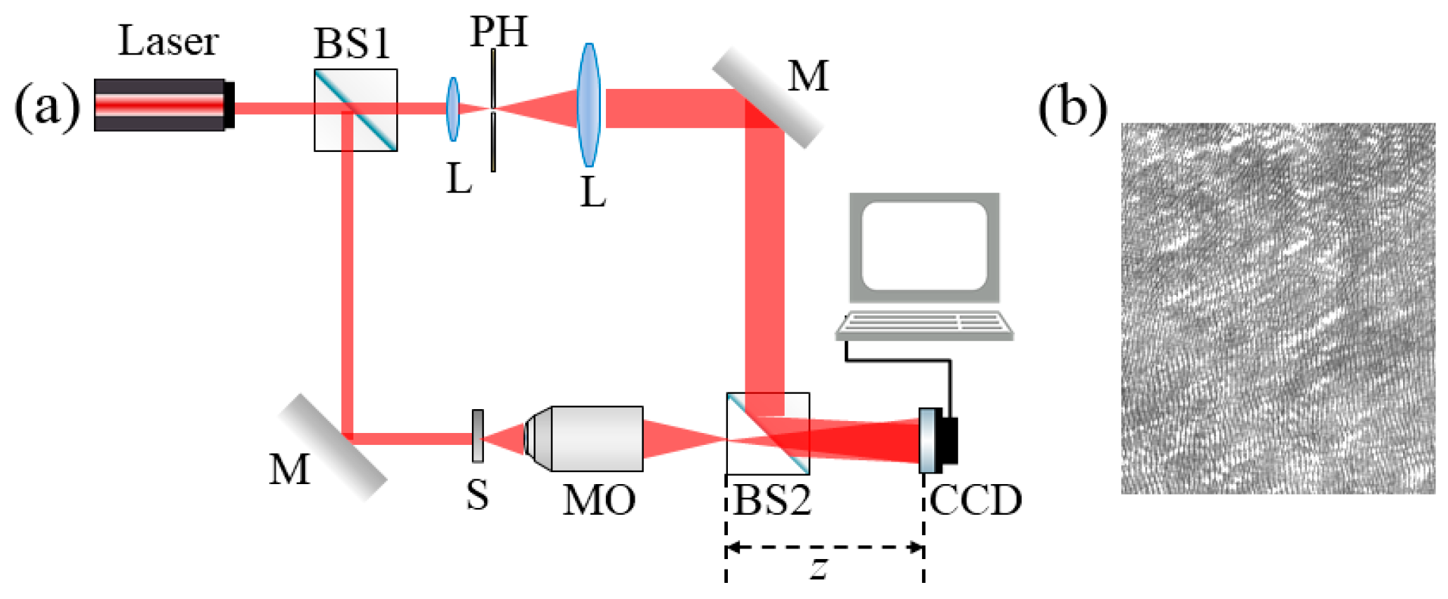
2. Off-Axis Digital Fresnel Hologram Reconstruction

In digital holography, the discretized digital hologram, denoted as I(p,q), can be formulated as follows,

$$I\left(p,q\right)=I(x,y)\times rect({\displaystyle \frac{x}{L_x}},{\displaystyle \frac{y}{L_y}})\times \sum _{p=1}^M\sum _{q=1}^N\delta (x-p\Delta x,y-q\Delta y)$$

(1)

where I(x,y) denotes the light intensity distribution of the hologram generated by the mutual interference between the object light and the reference light. M and N denote the number of pixels on the CCD plane in the x and y directions, respectively, with 1 ≤ p ≤ M and 1 ≤ q ≤ N. L_x and L_y denote the sizes of the CCD in the x and y directions, respectively. Δx and Δy denote the size of a single pixel on the CCD in the x and y directions, respectively. The relationships between these parameters are L_x = MΔx and L_y = NΔy. The last term δ(x−p∆x, y−q∆y) denotes a 2D Dirac comb function (also called sampling function). This describes a regular sampling grid in a 2D plane with intervals (Δx, Δy), generating a discrete array of sampling points. When the holographic optical recording conditions satisfy the Fresnel approximation conditions, the Fresnel approximation can be utilized to conduct numerical calculations on digital holograms, yielding a digital expression for the light intensity distribution on the reconstructed image plane,

$$\phi \left(m,n,z\right)={\displaystyle \frac{exp(i2\pi z/\lambda )}{i\lambda z}}exp\left\{i\pi \lambda z[{\left({\displaystyle \frac{x}{L_x}}\right)}^2+{\left({\displaystyle \frac{y}{L_y}}\right)}^2]\right\}FT\{I(p,q)R(p,q)exp\{{\displaystyle \frac{i\pi }{\lambda z}}[{(p\Delta x)}^2+{(q\Delta y)}^2]\}$$

(2)

where z represents the reconstruction distance, and 1 ≤ m ≤ M and 1 ≤ n ≤ N. FT{} represents the two-dimensional Fourier transform operation. During the digital hologram reconstruction process, the digital reference light used for numerical reconstruction is set as R(p,q) = 1. In simulations, when z equals the object distance (i.e., the distance from the object plane to the CCD detection plane during the recording process, the reconstructed image will be an ideally focused image. The various digital holographic autofocus methods mentioned earlier address the problem of how to find the ideal z-value. The light intensity distribution of the reconstructed image can be obtained by taking the modulus of the left-hand side of the above equation,

$$I\left(m,n,z\right)=\left|\phi (m,n,z)\right|$$

(3)

In DH, the reconstructed image consists of three components: the real image, the conjugate image, and the zero-order image. For off-axis Fresnel holographic optical paths, these three components can be well spatially separated when the angle between the reference light and the object optical axis satisfies the condition: θ ≥ (3D/2z), where D is the width of the object and z is the object distance. If this condition is not met, the three components will spatially overlap, resulting in a blurred reconstructed image. Additionally, in off-axis DH, if the reconstruction distance z used for numerical reconstruction does not match the distance between the object and the CCD during the hologram recording process, the reconstructed image will not be focused, resulting in a blurred image [33,34,35]. By introducing a microscope objective into the off-axis digital holographic recording optical configuration, it can be transformed into off-axis DHM, enabling the recording of digital holograms of microscopic objects. The numerical reconstruction of the hologram can also be achieved by Equation (2). Similarly, one of the key issues that needs to be addressed in off-axis DHM is how to quantitatively obtain the reconstruction distance of digital holograms, thereby achieving high-quality reconstructed image.

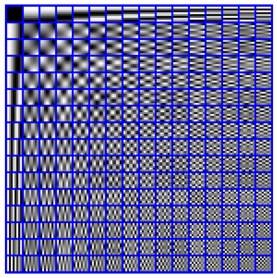
3. Basic Principle and Process of Denoising Image Through the DCT Dictionary

The basic principle and process of image denoising through the combination of the DCT dictionary and the OMP algorithm are as follows [33,36]. (1) The DCT dictionary construction: the DCT is a commonly used image transformation method that converts images from the spatial domain to the frequency domain. In image denoising, the coefficients resulting from the DCT transformation serve as the atoms of the dictionary, representing fundamental patterns of different frequency components within the image. The atoms of a fixed DCT dictionary are directly derived from the basis functions of the DCT transformation, which are typically predefined and do not vary with the image content. In this paper, an over-complete dictionary with a redundancy of 4 is employed, consisting of 256 atoms, resulting in a dictionary size of 64 × 256. The DCT dictionary used in this paper is shown in Figure 1. Blue grid cells are used to represent the decomposition of an augmented image into 256 atoms, with each grid cell representing one atom. Each of its atoms shown as an 8 × 8 pixel image. (2) Image blocking: the noisy image is segmented into multiple overlapping small blocks. In this paper, the image is partitioned into 8 × 8 blocks for processing. (3) Sparse coding: for each image block, the optimized orthogonal matching pursuit (OMP) algorithm is employed in conjunction with the DCT fixed dictionary to perform sparse coding, thereby identifying the optimal sparse representation coefficients. OMP is a greedy algorithm designed to solve the problem of sparse representation coefficients. OMP iteratively selects dictionary atoms that best match the current residual to gradually approximate the original signal. During each iteration, the OMP updates the residual and selects the atom from the remaining dictionary that is most correlated with the current residual. This process continues until a stopping criterion is met, such as achieving a predetermined sparsity level or when the residual falls below a certain threshold. (4) Image blocks reconstructing: each image block is reconstructed using the sparse representation coefficients and the DCT dictionary. These image blocks are stitched together to form a complete denoised image.

4. Focus Evaluation Function: The Edge Preservation Index

The autofocusing evaluation function generally serves as the standard for assessing the image clarity. The edge preservation index (EPI) is an important metric for evaluating the edge preservation capability of an image [37]. The EPI is defined as the ratio of the edge intensity along the horizontal direction in the denoised image to that in the original image, as illustrated in Equation (4). D(i,j) represents the denoised image. O(i,j) represents the original image. In this paper, the EPI is calculated and used as the vertical coordinate value of the obtained focus curve.

$${\mathrm{E}\mathrm{P}\mathrm{I}}_{\mathrm{H}}={\displaystyle \frac{\sum _{i=1}^{300}\sum _{j=1}^{200}\left|\mathrm{D}\left(\mathrm{i}+1,\mathrm{j}\right)-\mathrm{D}\left(\mathrm{i},\mathrm{j}\right)\right|}{\sum _{i=1}^{300}\sum _{j=1}^{200}\left|\mathrm{O}\left(\mathrm{i}+1,\mathrm{j}\right)-\mathrm{O}\left(\mathrm{i},\mathrm{j}\right)\right|}}$$

(4)

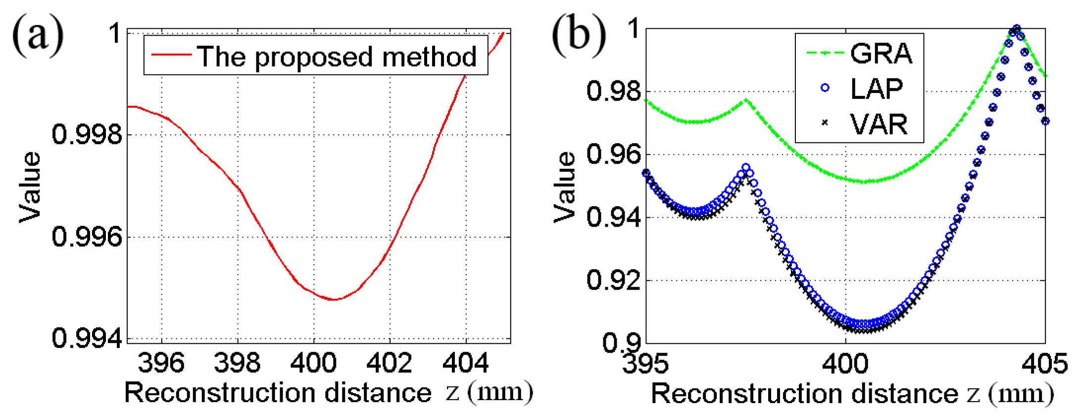
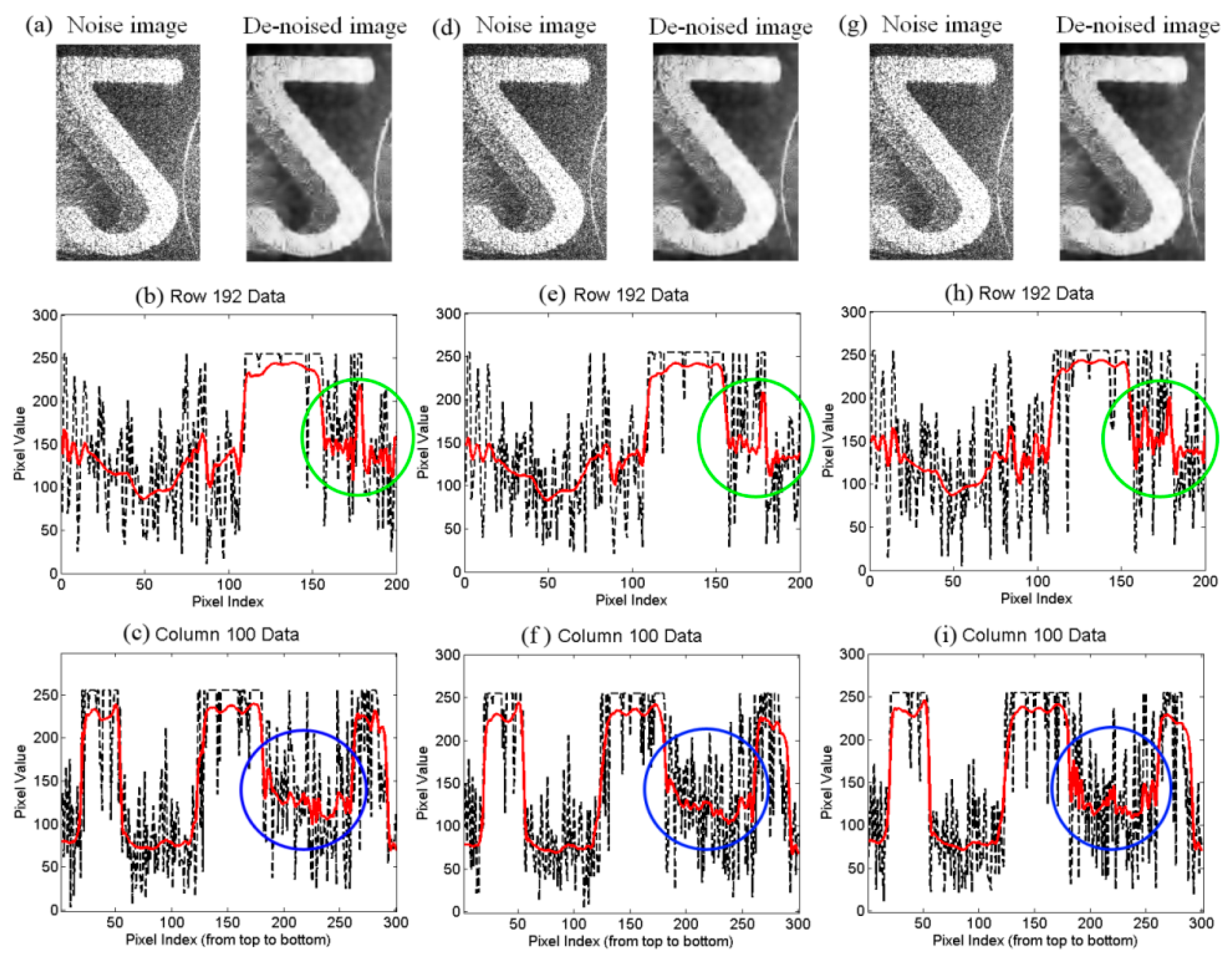
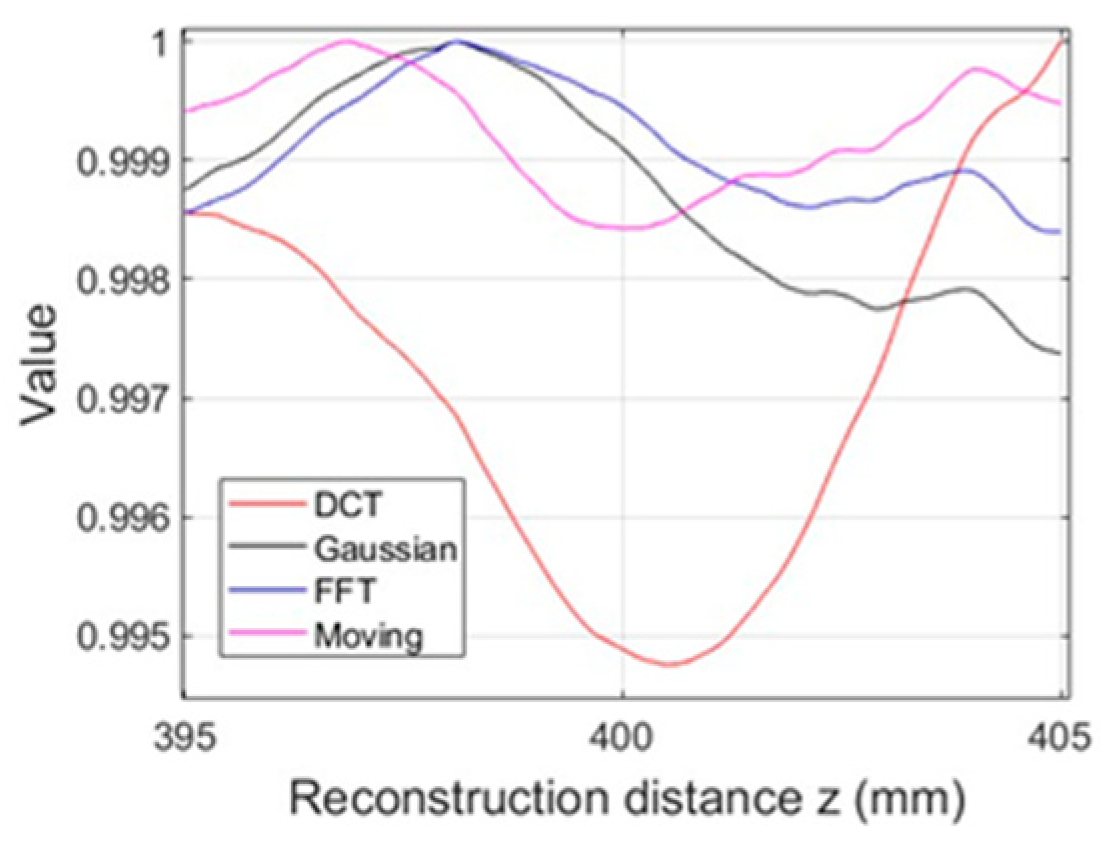
5. Results and Analysis

Figure 2a illustrates the optical configuration of the transmission-type off-axis DHM used in this paper. The light source is a He-Ne laser with a wavelength of 632.8 nm. The laser beam is split into two paths by a beam splitter (BS1). One path is expanded and collimated into a plane wave, serving as the reference light. The other path illuminates the micro-object (S denotes the sample), which is then magnified by microscope objective (MO) to form the object light. The reference light and the object light are converged by a polarizing beam splitter (BS2), with the reference light reaching the CCD plane at a slight incident angle relative to the object optical axis of the object light. The interference between the object and reference lights results in an off-axis digital hologram, as shown in Figure 2b. The parameters of the CCD camera include: a resolution of 756 × 572 pixels, a pixel size of 8.6 μm × 8.3 μm, and a sensing area of 6.4 mm × 4.8 mm. The microscopic object is a digit from a resolution test chart. A commercial MO with 10 × 0.25 NA is employed to generate a magnified image. In the experiment, the magnified image is positioned between the MO and the CCD plane, at a distance z in front of the CCD (as shown in Figure 2a). In the process of numerical reconstruction, if the reconstruction distance is set equal to z, a focused reconstructed image can be achieved. Furthermore, due to the configuration of the off-axis digital holographic optical path, it is convenient to filter out the conjugate image and zero-order image in the reconstructed image through frequency domain filtering techniques, thereby only obtaining the real image of the recorded object.

The process of obtaining the focus curve is as follows. Firstly, a sequence of reconstructed images is generated along the direction of light propagation at precise intervals of 0.1 mm within the search range of 10 mm. Synchronously, each reconstructed image undergoes efficient noise reduction processing using the DCT dictionary, resulting in a series of optimized, noise-reduced image sets corresponding to different reconstruction distances. On this basis, the EPI value between the denoised image and the original image at each reconstruction distance is calculated and used as the vertical coordinate of the focus curve. Next, a continuous graph is plotted, depicting the relationship between the EPI values and their respective reconstruction distances, to create an automatic focus curve.

Figure 3a presents the obtained autofocus curve for the off-axis digital holographic microscopic reconstructed image. It can be observed that, with a step size of 0.1 mm and within a search range of 10 mm, the resulting focus curve exhibits good unimodality. The optimal focus distances extracted from the minimum values of the focus curves is 400.5 mm. For comparison, Figure 3b presents the focus curves obtained using three other focusing methods. The definitions of these three focus functions can be found in Equations (5)–(7). Among them, VAR stands for the variance of gray value distribution, GRA represents the absolute gradient computation, and LAP denotes the Laplacian filtering algorithm [14]. VAR, GRA, and LAP exhibit fundamental differences in their operational principles. VAR quantifies global contrast through intensity dispersion. GRA measures edge sharpness via gradient magnitudes. LAP characterizes textural details using second-order derivatives.

$$\mathrm{V}\mathrm{A}\mathrm{R}={\displaystyle \frac{1}{\mathrm{M}\mathrm{N}}}{\sum }_{\mathrm{m}=1}^{\mathrm{M}}{\sum }_{\mathrm{n}=1}^{\mathrm{N}}{[\mathrm{I}\left(\mathrm{m},\mathrm{n}\right)-\overline{\mathrm{I}}]}^2,$$

(5)

$$\mathrm{G}\mathrm{R}\mathrm{A}={\sum }_{\mathrm{m}=2}^{\mathrm{M}}{\sum }_{\mathrm{n}=2}^{\mathrm{N}}\sqrt{{[\mathrm{I}\left(\mathrm{m},\mathrm{n}\right)-\mathrm{I}(\mathrm{m}-1,\mathrm{n}\left)\right]}^2+{[\mathrm{I}\left(\mathrm{m},\mathrm{n}\right)-\mathrm{I}(\mathrm{m},\mathrm{n}-1\left)\right]}^2},$$

(6)

$$\mathrm{L}\mathrm{A}\mathrm{P}={\sum }_{\mathrm{m}=2}^{\mathrm{M}}{\sum }_{\mathrm{n}=2}^{\mathrm{N}}{[\mathrm{I}\left(\mathrm{m}+1,\mathrm{n}\right)+\mathrm{I}\left(\mathrm{m}-1,\mathrm{n}\right)+\mathrm{I}\left(\mathrm{m},\mathrm{n}+1\right)+\mathrm{I}\left(\mathrm{m},\mathrm{n}-1\right)-4\mathrm{I}(\mathrm{m},\mathrm{n}\left)\right]}^2.$$

(7)

As can be seen from Figure 3b, with a step size of 0.1 mm and within a search range of 10 mm, these three focus curves exhibit multiple peaks, failing to meet the criteria of unimodality. Generally speaking, the focus evaluation curve needs to meet the criteria of unimodality and convergence. The optimal focus distances extracted from the minimum values of the focus curves corresponding to the VAR, GRA, and LAP evaluation functions are 400.6 mm, 400.5 mm, and 400.7 mm, respectively. In contrast, the focus curve derived from the focus evaluation function proposed in this paper exhibits good unimodality.

To further explain why the focus curves obtained exhibit unimodality characteristics, and to provide a comprehensive comparison of the image quality of the reconstructed images before and after noise reduction, the synthesis results are given in Figure 4. Figure 4a,d and g show the reconstructed images of the off-axis DHM before and after noise reduction, when the reconstruction distance z is set to 396 mm, 400.5 mm and 404 mm, respectively. Among them, z = 400.5 mm is the optimal reconstruction distance obtained by the proposed focusing algorithm in this paper. By comparing the noise image and denoised image shown in Figure 4a,d,g, a notable enhancement image quality in denoised image can be seen, including the preservation of details, sharpening of edges, and significant reduction in noise. The data corresponding to row 192 and column 100 in Figure 4a,d,g are extracted and plotted as graphs to illustrate the detailed changes in the images along the horizontal and vertical directions. Specifically, the curve data in Figure 4b,c are derived from Figure 4a. The curve data in Figure 4e,f are derived from Figure 4d. The curve data in Figure 4h,i are derived from Figure 4g. Among them, the black dashed line represents the data of noise image, while the red solid line represents the data of denoised image. These graphs provide a detailed analysis of the local features of the reconstructed images before and after noise reduction at each reconstruction distance. For instance, comparing the black and red curves, the black curve exhibits many random fluctuations (i.e., caused by noise), while the red curve is much smoother. These validate the effectiveness of the DCT dictionary learning-based image denoising method.

Next, let us analyze the red solid line data and black dashed line data within the green circles in Figure 4b,e,h, as well as the red solid line data and black dashed line data within the blue circles in Figure 4c,f,i. It can be observed that the red lines at the optimal reconstruction distance of z = 400.5 mm (see Figure 4e,f) exhibit a smoother profile with less fluctuation compared to the red lines at z = 396 mm (see Figure 4b,c) and z = 404 mm (see Figure 4h,i). This indicates that at the optimal reconstruction distance of z = 400.5 mm, not only a focused reconstructed image is obtained, but also a reconstructed image with better noise reduction is achieved. Consequently, the overall image quality of the reconstructed image is enhanced. At the same time, it should also be noted that: In Figure 4, there are saturated pixel values in the black dashed curve. This saturation may affect the quality or stability of the denoised result. However, the main purpose of this study is to achieve the focus of the reconstructed image and obtain the optimal reconstruction distance. For the denoising problem, in practical operation, the saturation problems can be effectively alleviated by combining dynamic range adjustment, anisotropic filtering, and post correction.

Once again, further analysis is conducted on the data represented by the red solid line and black dashed line shown in Figure 4b,e,h. Due to the smoother nature of the red curve and the higher randomness of the black curve’s fluctuations, at the optimal focus position (z = 400.5 mm), the differences between adjacent pixels along the horizontal direction in the denoised image are generally much smaller than those in the original noise image. According to Equation (4), the EPI defined in this paper is the ratio of the edge intensity along the horizontal direction in the denoised image to that in the original image before denoising. Their ratio will be slightly smaller or relatively smaller. However, at other reconstruction distances (e.g., z = 396 mm and z = 404 mm), the reconstructed image itself is blurred, and even after denoising, the image remains blurred. Consequently, it can be seen that the extracted red and black curves will both have many random fluctuations, as shown in Figure 4b,h. According to Equation (4), their ratio will be somewhat or relatively larger. Therefore, the curve obtained in this paper exhibits a minimum value within the search range.

By combining EPI focus evaluation function with various denoising algorithms, including the DCT-based denoising algorithm, the Gaussian denoising algorithm, the FFT denoising algorithm, and the moving average algorithm, the resulting focusing curves are given in Figure 5 [38,39,40]. It can be seen from Figure 5 that the focus curve obtained by combining the DCT-based filtering algorithm with the EPI criterion has unimodal characteristics, presents a U-shaped distribution, and has a large range of focus function values. However, the focus curves generated by integrating other denoising algorithms with the EPI criterion lack this crucial unimodal characteristic. This is mainly due to the fact that the DCT denoising algorithm can preserve more edge information of the denoised image. Therefore, Figure 5 effectively demonstrates the advantages of the focusing algorithm proposed in this paper, which combines the DCT denoising algorithm with the EPI criterion.

In brief, the experimental results indicate that, with a step size of 0.1 mm and within a broader search range of 10 mm, the obtained focusing evaluation curve exhibits better unimodality, and simultaneously a noise-reduced reconstructed image is achieved in DHM. This is the greatest advantage of the focus evaluation function proposed in this paper.

6. Conclusions

This paper proposes an automatic focusing scheme for off-axis DHM that combines the DCT dictionary with edge preservation index criteria. The fundamental process comprises several key steps. Firstly, a sequence of reconstruction images is generated at precise intervals within a predefined distance search range. Synchronously, speckle noise reduction is performed using DCT dictionaries and the OMP algorithm. Next, the EPI, which quantifies the ratio of edge intensity between the denoised and original images, is calculated and serves as a critical indicator for focus evaluation. Finally, an automatic focusing curve is constructed by plotting the EPI against the reconstruction distance, enabling the precise localization of the optimal focus position. The focusing curve obtained in this paper exhibits a good unimodality within the search range 10 mm with a step size of 0.1 mm. Once the optimal focus position is determined, a noise-reduced and focused reconstructed image can be simultaneously obtained.

This paper attempts to utilize noise reduction methods for autofocusing, in conjunction with a certain focusing evaluation function, to achieve automatic focusing of reconstructed images in DHM. By incorporating the DCT fixed dictionary to reduce speckle noise of the reconstructed images, and calculating the EPI between the denoised and original images as an evaluation metric, a single-peak focusing curve is obtained, enabling the determination of the optimal reconstruction distance in DHM. In end, both the automatic focused and denoised reconstructed images are achieved. This may be crucial for subsequent image analysis and processing tasks.

References

1. Anand, V.; Tahara, T.; Lee, W.M. Advanced optical holographic imaging technologies. Appl. Phys. B 2022, 128, 198. [Google Scholar] [CrossRef]
2. Li, S.; Kner, P.A. Optimizing self-interference digital holography for single-molecule localization. Opt. Express 2023, 31, 29352–29367. [Google Scholar] [CrossRef] [PubMed]
3. Zhang, J.; Dai, S.; Ma, C.; Xi, T.; Di, J.; Zhao, J. A review of common-path off-axis digital holography: Towards high stable optical instrument manufacturing. Light Adv. Manuf. 2021, 2, 333–349. [Google Scholar] [CrossRef]
4. Ghosh, A.; Noble, J.; Sebastian, A.; Das, S.; Liu, Z. Digital holography for non-invasive quantitative imaging of two-dimensional materials. J. Appl. Phys. 2020, 127, 084901. [Google Scholar] [CrossRef]
5. Huang, J.; Cai, W.; Wu, Y.; Wu, X. Recent advances and applications of digital holography in multiphase reactive/nonreactive flows: A review. Meas. Sci. Technol. 2021, 33, 022001. [Google Scholar] [CrossRef]
6. Li, T.; Wu, Y.; Wu, X. Morphology and position measurement of irregular opaque particle with digital holography of side scattering. Powder Technol. 2021, 394, 384–393. [Google Scholar] [CrossRef]
7. Di, J.; Song, Y.; Xi, T.; Zhang, J.; Li, Y.; Ma, C.; Wang, K.; Zhao, J. Dual-wavelength common-path digital holographic microscopy for quantitative phase imaging of biological cells. Opt. Eng. 2017, 56, 111712. [Google Scholar] [CrossRef]
8. Huang, J.; Li, S.; Zi, Y.; Qian, Y.; Cai, W.; Aldén, M.; Li, Z. Clustering-based particle detection method for digital holography to detect the three-dimensional location and in-plane size of particles. Meas. Sci. Technol. 2021, 32, 055205. [Google Scholar] [CrossRef]
9. Trusiak, M.; Picazo-Bueno, J.A.; Zdankowski, P.; Micó, V. DarkFocus: Numerical autofocusing in digital in-line holographic microscopy using variance of computational dark-field gradient. Opt. Laser Eng. 2020, 134, 106195. [Google Scholar] [CrossRef]
10. Tang, M.; Liu, C.; Wang, X.P. Autofocusing and image fusion for multi-focus plankton imaging by digital holographic microscopy. Appl. Opt. 2020, 59, 333–345. [Google Scholar] [CrossRef]
11. Wen, Y.; Wang, H.; Anand, A.; Qu, W.; Cheng, H.; Dong, Z.; Wu, Y. A fast autofocus method based on virtual differential optical path in digital holography: Theory and applications. Opt. Laser Eng. 2019, 121, 133–142. [Google Scholar] [CrossRef]
12. Ou, H.; Wu, Y.; Lam, E.Y.; Wang, B.Z. New autofocus and reconstruction method based on a connected domain. Opt. Lett. 2018, 43, 2201–2203. [Google Scholar] [CrossRef] [PubMed]
13. Memmolo, P.; Paturzo, M.; Javidi, B.; Netti, P.A.; Ferraro, P. Refocusing criterion via sparsity measurements in digital holography. Opt. Lett. 2014, 39, 4719–4722. [Google Scholar] [CrossRef] [PubMed]
14. Langehanenberg, P.; Kemper, B.; Dirksen, D.; Von Bally, G. Autofocusing in digital holographic phase contrast microscopy on pure phase objects for live cell imaging. Appl. Opt. 2008, 47, D176–D182. [Google Scholar] [CrossRef]
15. Long, J.; Yan, H.; Li, K.; Zhang, Y.; Pan, S.; Cai, P. Autofocusing by phase difference in reflective digital holography. Appl. Opt. 2022, 61, 2284–2292. [Google Scholar] [CrossRef] [PubMed]
16. Zhang, Y.; Wang, H.; Wu, Y.; Tamamitsu, M.; Ozcan, A. Edge sparsity criterion for robust holographic autofocusing. Opt. Lett. 2017, 42, 3824–3827. [Google Scholar] [CrossRef]
17. Fatih Toy, M.; Kühn, J.; Richard, S.; Parent, J.; Egli, M.; Depeursinge, C. Accelerated autofocusing of off-axis holograms using critical sampling. Opt. Lett. 2012, 37, 5094–5096. [Google Scholar] [CrossRef]
18. Zhang, Y.; Huang, Z.; Jin, S.; Cao, L. Hough transform-based multi-object autofocusing compressive holography. Appl. Opt. 2023, 62, D23–D30. [Google Scholar] [CrossRef]
19. Ghosh, A.; Kulkarni, R.; Mondal, P.K. Autofocusing in digital holography using eigenvalues. Appl. Opt. 2021, 60, 1031–1040. [Google Scholar] [CrossRef]
20. Zhang, Y.; Huang, Z.; Jin, S.; Cao, L. Autofocusing of in-line holography based on compressive sensing. Opt. Laser Eng. 2021, 146, 106678. [Google Scholar] [CrossRef]
21. Ren, Z.; Xu, Z.; Lam, E.Y. Learning-based nonparametric autofocusing for digital holography. Optica 2018, 5, 337–344. [Google Scholar] [CrossRef]
22. Lin, W.; Chen, L.; Chen, Y.; Cai, W.; Hu, Y.; Wen, K. Single-shot speckle reduction by elimination of redundant speckle patterns in digital holography. Appl. Opt. 2020, 59, 5066–5072. [Google Scholar] [CrossRef]
23. Bianco, V.; Memmolo, P.; Leo, M.; Montresor, S.; Distante, C.; Paturzo, M.; Picart, P.; Javidi, B.; Ferraro, P. Strategies for reducing speckle noise in digital holography. Light Sci. Appl. 2018, 7, 48. [Google Scholar] [CrossRef] [PubMed]
24. Bianco, V.; Memmolo, P.; Paturzo, M.; Finizio, A.; Javidi, B.; Ferraro, P. Quasi noise-free digital holography. Light Sci. Appl. 2016, 5, e16142. [Google Scholar] [CrossRef] [PubMed]
25. Hincapie, D.; Herrera-Ramírez, J.; Garcia-Sucerquia, J. Single-shot speckle reduction in numerical reconstruction of digitally recorded holograms. Opt. Lett. 2015, 40, 1623–1626. [Google Scholar] [CrossRef] [PubMed]
26. Ibrahim, D.G.A. Improving the intensity-contrast image of a noisy digital hologram by convolution of Chebyshev type 2 and elliptic filters. Appl. Opt. 2021, 60, 3823–3829. [Google Scholar] [CrossRef]
27. Chen, K.; Chen, L.; Xiao, J.; Li, J.; Hu, Y.; Wen, K. Reduction of speckle noise in digital holography using a neighborhood filter based on multiple sub-reconstructed images. Opt. Express 2022, 30, 9222–9232. [Google Scholar] [CrossRef]
28. Montrésor, S.; Memmolo, P.; Bianco, V.; Ferraro, P.; Picart, P. Comparative study of multi-look processing for phase map de-noising in digital Fresnel holographic interferometry. J. Opt. Soc. Am. A 2019, 36, A59–A66. [Google Scholar] [CrossRef]
29. Fang, Q.; Xia, H.; Song, Q.; Zhang, M.; Guo, R.; Montresor, S.; Picart, P. Speckle denoising based on deep learning via a conditional generative adversarial network in digital holographic interferometry. Opt. Express 2022, 30, 20666–20683. [Google Scholar] [CrossRef]
30. Yan, K.; Chang, L.; Andrianakis, M.; Tornari, V.; Yu, Y. Deep learning-based wrapped phase denoising method for application in digital holographic speckle pattern interferometry. Appl. Sci. 2020, 10, 4044. [Google Scholar] [CrossRef]
31. Montresor, S.; Tahon, M.; Laurent, A.; Picart, P. Computational de-noising based on deep learning for phase data in digital holographic interferometry. APL Photonics 2020, 5, 030802. [Google Scholar] [CrossRef]
32. Zeng, T.; Zhu, Y.; Lam, E.Y. Deep learning for digital holography: A review. Opt. Express 2021, 29, 40572–40593. [Google Scholar] [CrossRef] [PubMed]
33. Lin, Z.; Jia, S.; Zhou, X.; Zhang, H.; Wang, L.; Li, G.; Wang, Z. Digital holographic microscopy phase noise reduction based on an over-complete chunked discrete cosine transform sparse dictionary. Opt. Laser Eng. 2023, 166, 107571. [Google Scholar] [CrossRef]
34. Picazo-Bueno, J.A.; Trusiak, M.; Micó, V. Single-shot slightly off-axis digital holographic microscopy with add-on module based on beamsplitter cube. Opt. Express 2019, 27, 5655–5669. [Google Scholar] [CrossRef]
35. Reddy, B.L.; Ramachandran, P.; Nelleri, A. Optimal Fresnelet sparsification for compressive complex wave retrieval from an off-axis digital Fresnel hologram. Opt. Eng. 2021, 60, 073102. [Google Scholar] [CrossRef]
36. Elad, M.; Aharon, M. Image denoising via sparse and redundant representations over learned dictionaries. IEEE Trans. Image Process. 2006, 15, 3736–3745. [Google Scholar] [CrossRef]
37. Waske, B.; Braun, M.; Menz, G. A segment-based speckle filter using multisensoral remote sensing imagery. IEEE Geosci. Remote Sens. Lett. 2007, 4, 231–235. [Google Scholar] [CrossRef]
38. Ri, S.; Takimoto, T.; Xia, P.; Wang, Q.; Tsuda, H.; Ogihara, S. Accurate phase analysis of interferometric fringes by the spatiotemporal phase-shifting method. J. Opt. 2020, 22, 105703. [Google Scholar] [CrossRef]
39. Soncco, D.C.; Barbanson, C.; Nikolova, M.; Almansa, A.; Ferrec, Y. Fast and accurate multiplicative decomposition forfringe removal in interferometric images. IEEE Trans. Comput. Imaging 2017, 3, 187–201. [Google Scholar] [CrossRef]
40. Galaktionov, I.; Sheldakova, J.; Toporovsky, V.; Kudryashov, A. Modified fizeau interferometer with the polynomial and FFT smoothing algorithm. Proc. SPIE 2022, 12223, 6. [Google Scholar] [CrossRef]
Figure 1. The DCT dictionary used for noise reduction in this paper.
Optics 06 00017 g001
Figure 2. (a) The off-axis DHM optical configuration. BS: beam splitter, PH: pinhole, M: mirror, MO: microscope objective, and S: sample. z: object distance. (b) A portion of the obtained hologram.
Optics 06 00017 g002
Figure 3. The obtained autofocus curve for the reconstructed images in off-axis DHM. (a) corresponds to the DCT dictionary-based denoising with edge preservation index criteria method, and (b) corresponds to the VAR, GRA, and LAP evaluation functions.
Optics 06 00017 g003
Figure 4. Experimental results. (a), (d) and (g), respectively, show the reconstructed images of the off-axis DHM before and after noise reduction, when the reconstruction distance z = 396 mm, 400.5 mm and 404 mm. z = 400.5 mm is the optimal reconstruction distance obtained by the proposed focusing algorithm in this paper. (b), (e) and (h), respectively, show the data extracted from the 192nd row of the reconstructed images shown in (a,d,g). (c), (f) and (i), respectively, show the data extracted from the 100th column of the reconstructed images shown in (a,d,g). Among them, the black dashed line corresponds to the data of noise image, and the red solid line corresponds to the data of denoised image.
Optics 06 00017 g004
Figure 5. The focusing curves obtained by combining EPI with the DCT-based denoising algorithm, the Gaussian denoising algorithm, the FFT denoising algorithm, and the moving average algorithm.
Optics 06 00017 g005
Disclaimer/Publisher’s Note: The statements, opinions and data contained in all publications are solely those of the individual author(s) and contributor(s) and not of MDPI and/or the editor(s). MDPI and/or the editor(s) disclaim responsibility for any injury to people or property resulting from any ideas, methods, instructions or products referred to in the content.