Article

Theoretical Model of Curved Liquid Surface in the Microholes for Molding Microlenses

Engineering Research Center of Optical Instrument and System, The Ministry of Education, Shanghai Key Laboratory of Modern Optical System, University of Shanghai for Science and Technology, Shanghai 200093, China
*
Authors to whom correspondence should be addressed.
Optics 2025, 6(2), 13; https://doi.org/10.3390/opt6020013
Submission received: 8 February 2025 / Revised: 19 March 2025 / Accepted: 20 March 2025 / Published: 3 April 2025

Abstract

:
Microlenses are essential optics widely used in many fields. The microfluidics-assisted fabrication method provides a rapid, convenient way to manufacture microlenses. However, there is no mathematical model to describe the profile of the liquid surface. This paper provides a theoretical explanation and mathematical model for the formation of the liquid surface of different curvatures in the microholes of different shapes. A numerical model based on the finite–difference time–domain method verifies the mathematical model. Furthermore, the optical properties of the microlenses in different shapes are analyzed through the demolded microlenses. The proposed theoretical model provides an analytical way to study the properties of microlenses.

1. Introduction

Microlenses play an important role in micro-optical systems. Microlenses in different shapes realize the precise manipulation of light at the micro and nano scale through specific processing. They are small, lightweight, highly integrated, and have excellent optical properties. Microlenses in different shapes have a wide range of applications in many fields [1,2,3,4,5,6,7,8,9]. In fiber optic communications, microlenses in different shapes can be used for optical coupling, beam shaping, and optical path conversion to improve the transmission efficiency of the communication system [1,2]. In imaging and detection systems, microlenses in different shapes can be used to realize high-resolution imaging and fast target detection [3,4,5,6,7]. In biomedical fields, microlenses in different shapes can be used in laser surgery, skin aesthetics, and optical diagnostics. They can be used to make miniature endoscopes for in vivo observation and diagnosis to improve the precision and effectiveness of treatment [8,9].
There are several methods for fabricating microlenses [10,11,12,13,14,15,16,17,18,19,20,21,22,23,24,25,26,27,28,29,30]. In the thermal reflow method, photoresist cylinders are prepared on a substrate using the photolithography technique. Then, the cylindrical posts are heated. The photoresist is softened and reflows into a lens shape [10,11,12]. The laser direct writing method utilizes a variable-intensity laser beam to expose the photoresist coated on the substrate. After development, a microlens profile can be formed [13,14,15]. Two-photon polymerization 3D printing technology utilizes the simultaneous absorption of energy by two photons to stimulate a polymerization reaction in the photosensitive polymer. Complex structures can be precisely printed in three dimensions [16,17]. Reactive ion etching based on chemical reaction and physical bombardment mechanisms can also be applied for microlens fabrication [18,19]. Grayscale lithography utilizes a mask plate to realize variable-dose exposure on the different positions. Microstructures with different depths can be generated [20,21,22]. In recent years, the microfluidics-assisted fabrication method has been widely used in the fabrication of miniature optical devices [23,24,25,26,27,28,29]. The method harnesses gravitational force, viscous resistance, surface tension, and other external forces, e.g., spinning force, to manipulate the microfluid. By regulating the profile of the liquid surface, microlenses and microlens arrays can be efficiently generated.
Although the microfluidics-assisted fabrication method has been widely used in the fabrication of microlenses and microlens arrays, there are few studies on the theory of the method, especially the formation of the liquid profiles [23,24,25,26]. Herein, we developed numerical models and analytical models to explain the formation of the liquid profile in the microholes of different shapes. Three types of microhole models, i.e., cylindrical, square, and hexagonal microholes, are used in the simulation. We also derived the equations to calculate the liquid profiles in the cylindrical, square, and hexagonal microholes. The calculated results were validated with those obtained in the simulation using the numerical models. The 3D models of the microlenses with the profiles predicted by the proposed model were established, based on which of the optical properties were analyzed.

2. Design of Microlens in the Pre-Defined Microholes

There is a relationship between the contact angle formed by the photoresist and the microhole wall and the curvature of the microlens, as shown in Figure 1. By adjusting the contact angle between the photoresist in the microhole and the microhole wall, we can obtain microlenses with adjustable curvature [31]. The relationship between the contact angle θ formed by the photoresist and the microhole wall and the contact angle α of the microlens is shown in Equation (1).
α + θ = 90 ° ,
By adjusting the contact angle θ, we obtain microlenses with different contact angles α to realize the adjustable curvature. In the figure, h is the concave height of the microhole, and conversely, h indicates the convex height of the microlens. By adjusting the contact angle θ, the raised height of the microlens changes accordingly. In order to investigate different shapes of microlenses, we designed three shapes of microlens models: a round microlens model, a square microlens model, and a hexagonal microlens model. By modeling the rise of the liquid surface in the microholes, we can get the concave liquid surface under different contact angles. The microlenses with different contact angles are finally obtained to realize the adjustable curvature.

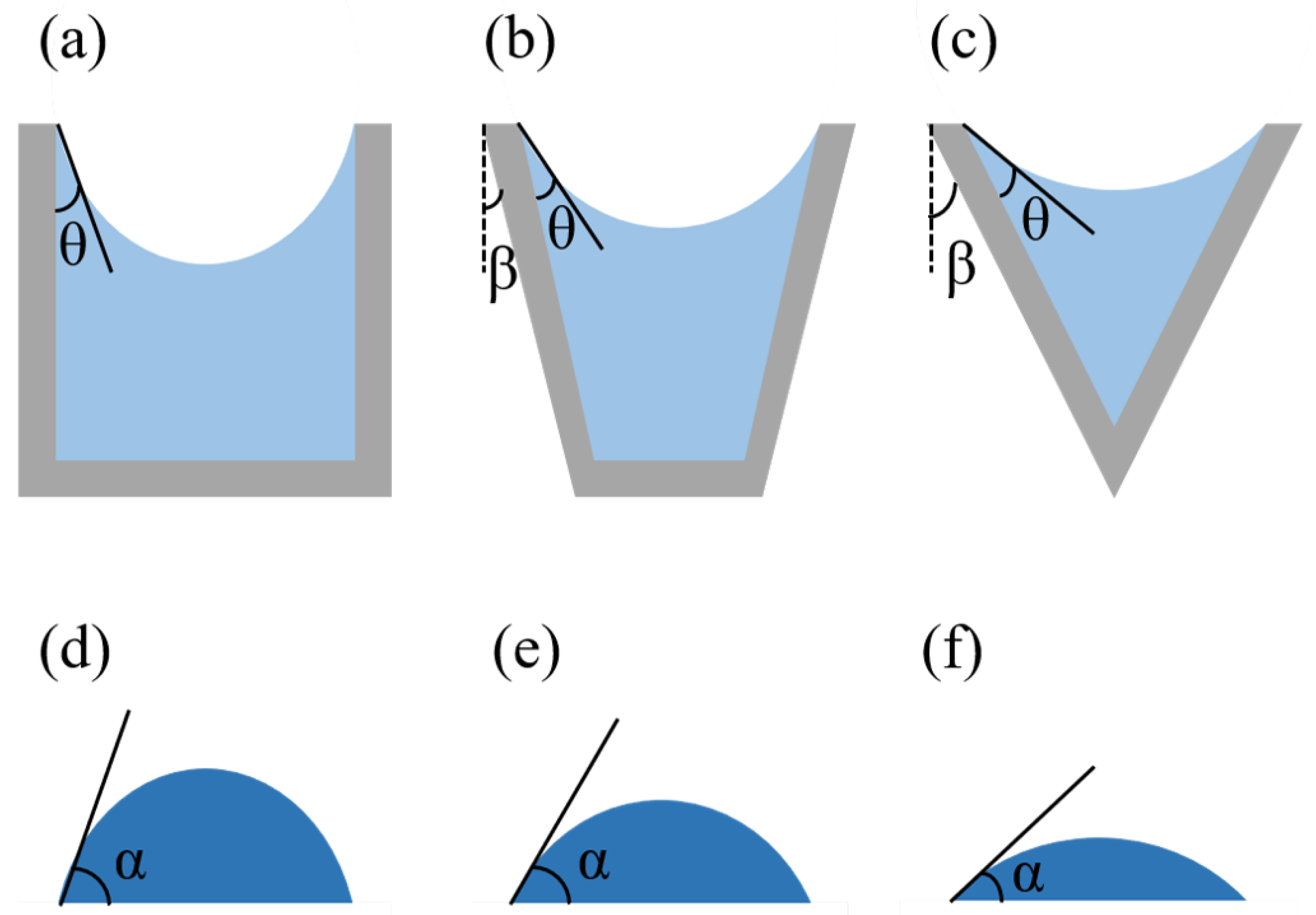
3. Models for the Formation of the Microlens Mold

3.1. Numerical Model Based on Finite–Difference Time–Domain (FDTD) Method

We built a numerical model using capillary filling models using the FDTD method in the COMSOL Multiphysics 6.0 software [32,33,34,35,36,37,38,39,40]. In order to investigate different shapes, we built three shapes of capillary filling models as a cylindrical model, a square model, and a hexagonal model.
We describe the cylindrical model in detail. We built a cylinder with a radius of 0.5 mm and a height of 8 mm. The cylinder was divided into upper and lower parts. The upper part was air and the lower part was liquid. Liquid rises through the channel due to wall adhesion and surface tension between the air and the liquid interface. The wall adhesion force causes the liquid to diffuse up along the side of the column wall, and the deformation of the liquid surface triggers the surface tension at the air–liquid interface. This leads to a sudden change in pressure above and below the interface. This pressure difference causes liquid and air to rise. The liquid continues to rise until the surface tension equilibrates with the gravitational force generated by the rising liquid in the channel. We used the “two-phase flow, phase field” Multiphysics field coupling feature in the microfluidics module to model the filling of the capillary. In the “Phase Field” interface, the two-phase flow dynamics was governed by the Cahn–Hilliard equation [41]. We use this equation to represent the diffusion interface separating the two phases. The model simulates the mass and momentum transfer of the fluid based on the Navier–Stokes equation for incompressible fluids [42]; in order to include the effect of surface tension, it must be included in the model.
Here, we present a detailed account of COMSOL simulations investigating liquid surface behavior within cylindrical microholes. The simulation framework was established by initiating a three-dimensional model in COMSOL Multiphysics software, utilizing the fluid flow module to configure multi-phase, two-phase, and laminar flow using the phase field method. A transient study with phase initialization was selected to capture dynamic interface evolution. The geometric model comprised two vertically aligned cylinders with a radius of 0.5 mm and a height of 4 mm merged into a unified structure, with material assignments differentiating the upper air domain from the lower SU8 polymer section. Boundary conditions were implemented with no-slip walls at the top and bottom extremities, while lateral surfaces employed Navier slip conditions using minimum cell length factors for slip length specification, excluding wall translation effects under friction. The fluid–fluid interface configuration incorporated prescribed contact angle parameters and wall–normal velocity constraints, complemented by pressure point constraints applied to four vertices of the upper cylinder. Mesh refinement was systematically executed through physics-controlled grid optimization to enhance resolution at critical interfaces. Transient simulations were conducted with adaptive solver parameter adjustments to address potential convergence challenges, including initialization inconsistencies, temporal step failures, and Newton–Raphson iteration limits. This comprehensive approach enabled robust numerical analysis of interfacial dynamics while maintaining computational stability throughout the simulation process.
By setting different angles of contact angle, we finally get the cylindrical liquid rise model with α of 10°, 20°, 30°, 40°, as shown in Figure 2.
By analogy, we can obtain the square liquid rise model, and the hexagonal liquid rise model, as shown in Figure 3 and Figure 4. We compare the numerical model simulated by COMSOL with the theoretical model derived from the equation.

3.2. Theoretical Model Based on Mathematical Derivation

For the theoretical model, through the derivation of the equation, we established the cylindrical surface model, the square surface model, and the hexagonal surface model. The theoretical model is based on the space xyz coordinate system. Through Equation (2), we can obtain the cylindrical surface model.
z = R 2 x 2 y 2 ,
where R = r c o s ( θ ) , r is the cylindrical radius, and θ is the contact angle. Since the liquid surface of the cylindrical surface model is a concave liquid surface, we chose the negative solution.
For the square surface model, the surface consists of a superposition of two surfaces. Since the square is formed by combining two sets of walls that are perpendicular to each other, the two surfaces contribute independently to the height of the curved moon surface [43]. Through the mathematical relationship of the concave liquid surface, as shown in Figure 5, we can obtain the equation of the surface. Establish a coordinate system at the lowest point of the lower concave liquid level, and Equations (3)–(5) show the process of calculating a parabolic surface. By using Equations (6)–(8), we can obtain the square surface model.
Z = a x 2 + b y + c ,   b   =   0 ,   c   =   0 ,
r c o s ( θ ) r t a n ( θ ) = a r 2 ,
a = 1 r c o s ( θ ) tan ( θ ) r ,
z 1 = ( 1 r c o s ( θ ) tan ( θ ) r ) x 2 ,
z 2 = ( 1 r c o s ( θ ) tan ( θ ) r ) y 2 ,
z = z 1 + z 2 = ( 1 r c o s ( θ ) tan ( θ ) r ) x 2 + ( 1 r c o s ( θ ) tan ( θ ) r ) y 2 ,
where r is the radius of the inscribed circle, and θ is the contact angle.
For the hexagonal surface model, the surface consists of three surfaces superimposed on each other. The three surfaces contribute to the height of the curved moon surface with certain weights. By using Equations (9)–(14), we can obtain the hexagonal surface model.
z 1 = ( 1 r cos ( θ ) tan ( θ ) r ) x 2 ,
x 2 = 1 2 x 3 2 y y 2 = 3 2 x + 1 2 y ,
z 2 = f ( x 2 , y 2 , z ) ,
x 3 = 1 2 x 3 2 y y 3 = 3 2 x 1 2 y ,
z 3 = f ( x 3 , y 3 , z ) ,
z = 1 3 z 1 + 1 3 z 2 + 1 3 z 3 ,
where r is the radius of the inscribed circle of the hexagonal, and θ is the contact angle.
By comparing the numerical model of the COMSOL simulation with the theoretical model derived from the equation, Figure 6 is obtained. The picture shows that the numerical model simulated by COMSOL is in general agreement with the theoretical model derived from the equation. Since the COMSOL simulation has some minor fluctuations in the liquid level, it is not perfectly symmetrical. The deviation is small—less than 0.5 microns. The relative error is small, and the absolute error is small. The absolute errors for the cylindrical model, the square model, and the hexagonal model are MSE1cylindrical = 1.4127 × 10 7 , MSE2square = 2.2677 × 10 8 , and MSE3hexagonal = 1.5498 × 10 8 , respectively. This shows that the theoretical model derived from the equation has a great degree of veracity.

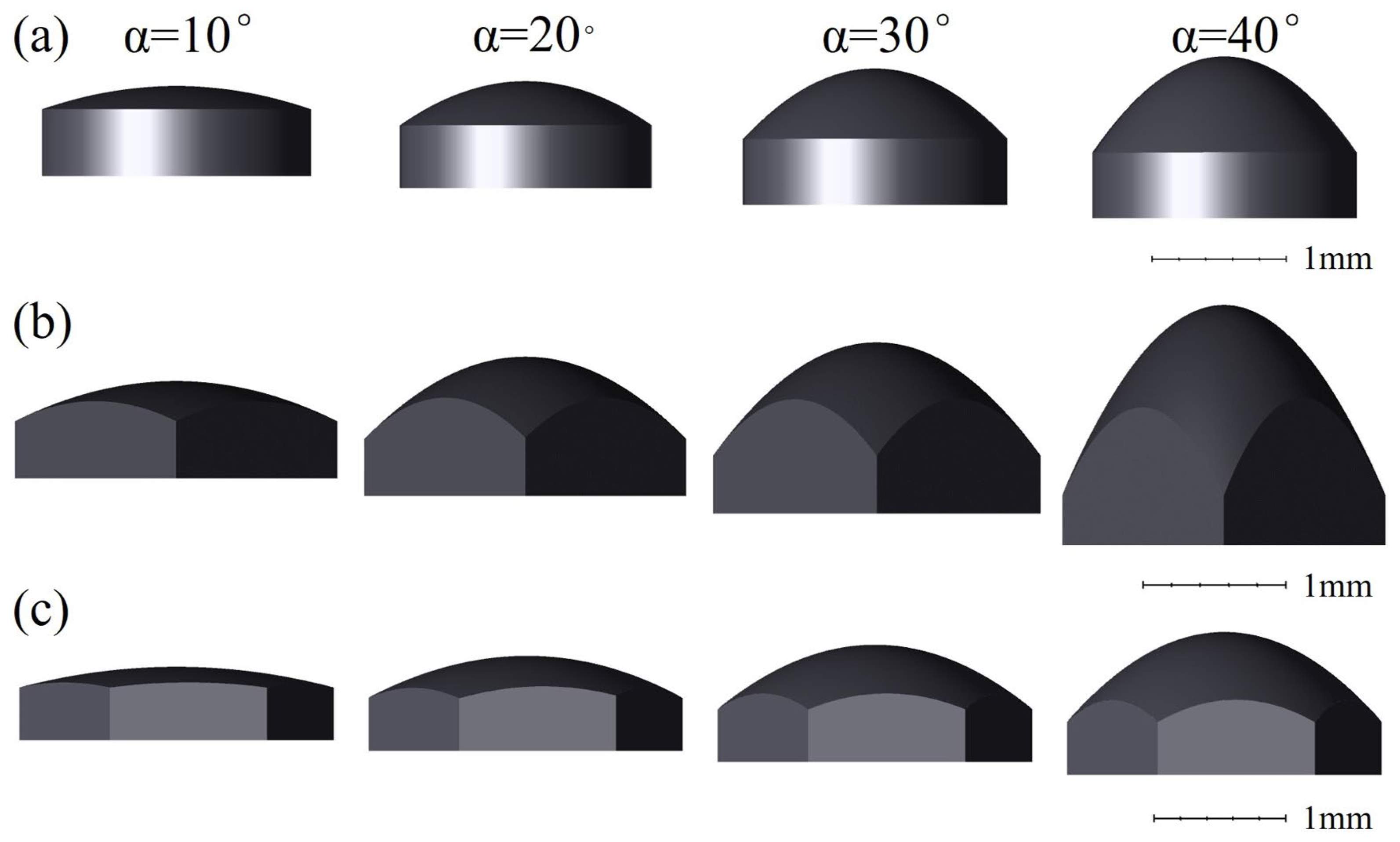
4. Profile of Microlens

Based on the theoretical model derived from the equation through MATLAB R2018b simulation, we derive the extended polynomial corresponding to the model, as shown in Equation (15). In Ansys Zemax OpticStudio, using the extended polynomial corresponding to the model, we can derive the profile of the microlens, as shown in Figure 7. The light propagated from top to bottom. The microlens’ thickness is 0.5 mm, and the material is BK7.
z = p 00 + p 10 x + p 01 y + p 20 x 2 + p 11 x y + p 02 y 2 ,

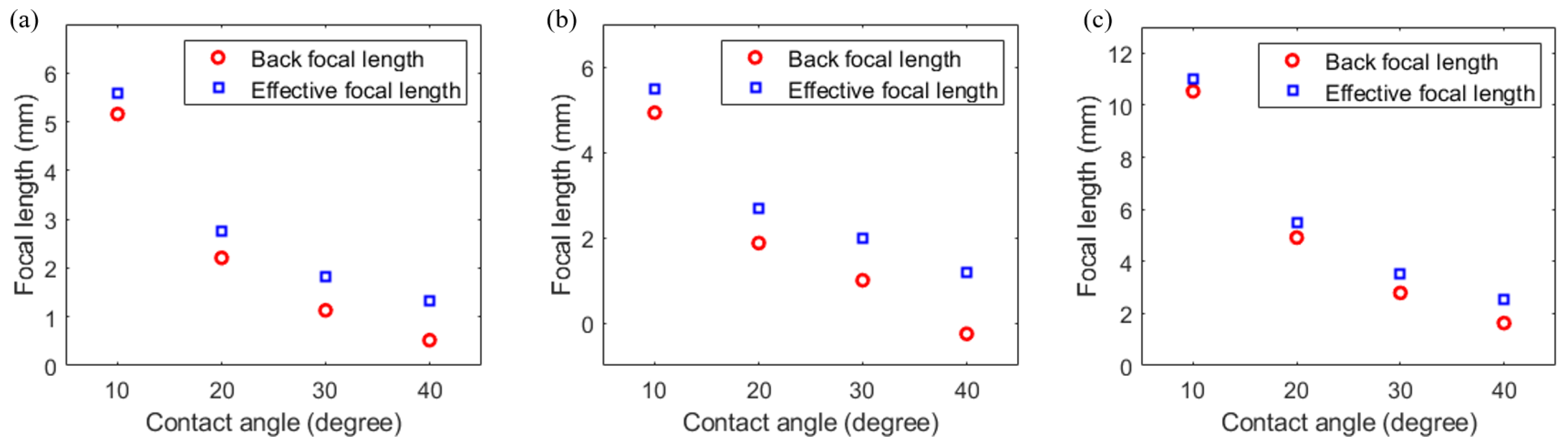
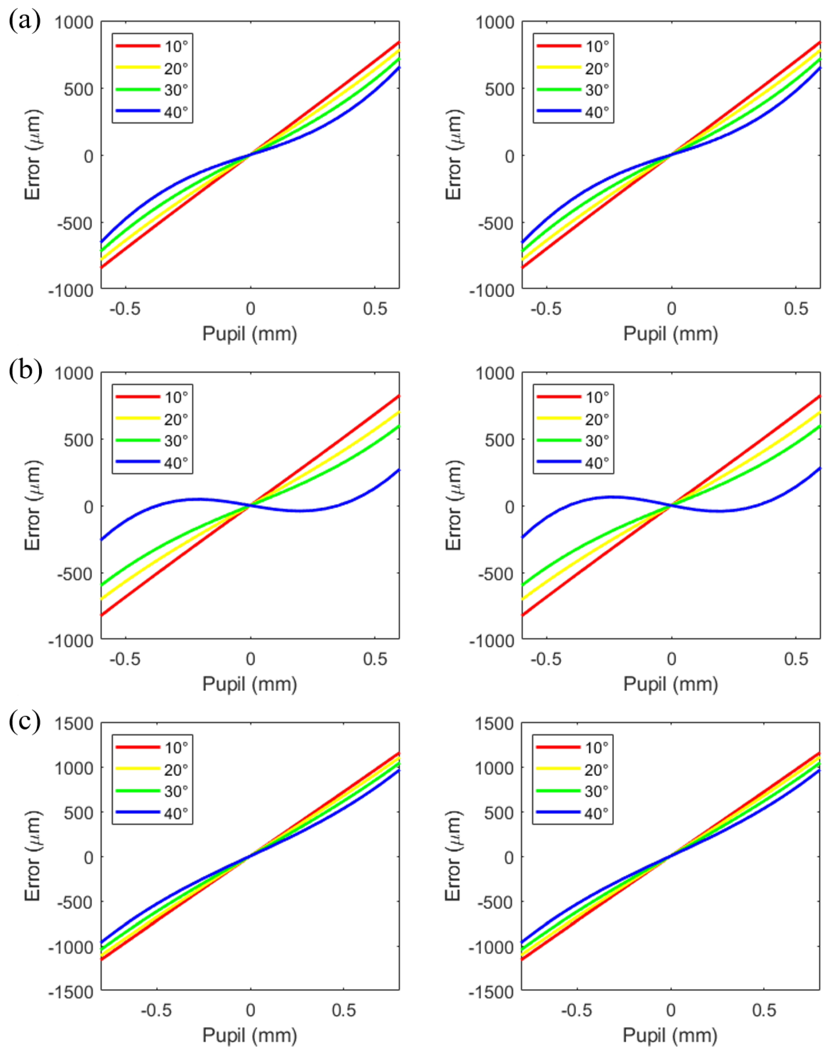
5. Optical Characteristics of the Microlens

The models of the microlenses are created using commercial optical design software, i.e., Ansys Zemax OpticStudio 2023. Then, we analyze the optical characteristics of the microlenses to realize the study of microlenses in different shapes.
The back focal length and the effective focal length are important parameters of a microlens, and they determine the ability of the lens to converge light rays and its imaging characteristics. The formulas for back focal length and effective focal length are shown in Equations (16)–(18).
B F L = f d n ,
where f is the effective focal length, n is the refractive index of the lens material, and d is the thickness of the lens.
1 f = ( n 1 ) ( 1 R 1 1 R 2 ) ,
where f is the effective focal length, n is the refractive index of the lens material, and R 1 and R 2 are the radius of curvature of the two surfaces of the lens, respectively. For plano-convex lenses, assuming that the radius of curvature of the plane side of the R 2 = , the formula simplifies to Equation (18).
f = R 1 n 1 ,
In addition, it has been suggested that exact equations for the back and effective focal lengths of a plano–concave thick lens are those shown in Equations (19) and (20) [44].
B F L = R ( 1 n n 2 1 n 2 1 ) ,
E F L = R n 2 1 n ( n 2 1 ) ,
where n is the refractive index of the lens material, and R is the radius of curvature of the surfaces of the lens.
First, we can obtain the back focal length and effective focal length of the microlens as shown in Figure 8. As the contact angle gradually increases, both the back focal length and effective focal length of the microlens gradually decrease. For the same range of contact angle variation, round microlenses and square microlenses have similar ranges of back focal length and effective focal length in Figure 8a,b, and hexagonal microlenses have wider ranges of back focal length and effective focal length in Figure 8c. The longer the effective focal length, the weaker the ability of the lens to converge light rays, and the smaller and farther away the image of the object will be when it is imaged.
For spherical aberration, we can obtain spherical aberration along the y-axis and spherical aberration along the x-axis, as shown in Figure 9. Compared to the spherical aberration along the y-axis and the spherical aberration along the x-axis of round microlenses in Figure 9a, Figure 9c shows hexagonal microlenses have a slightly bigger spherical aberration along the y-axis and spherical aberration along the x-axis. For different contact angles, the spherical aberration along the y-axis and the spherical aberration along the x-axis of square microlenses have a slightly more significant change. All three shapes of microlenses have small phase differences.
In addition, the meridional plane (which contains the optical axis of the lens) and the sagittal plane (which is vertical to the meridional plane) have different radiuses. Therefore, the meridional and sagittal rays have different focal points. This is called an astigmatism aberration. The spherical aberration along the y-axis and spherical aberration along the x-axis illustrated in Figure 9 are very similar, which suggests that the astigmatism aberration is small.
In addition, compared to the ideal lens, such as diffraction-limited, high-precision aspheric lens, as shown in Figure 10, their silhouettes overlap significantly. Our manufacturing method is simple and low-cost, but the profile of the lens is constrained by the surface formed in the microholes due to the range of contact angles.

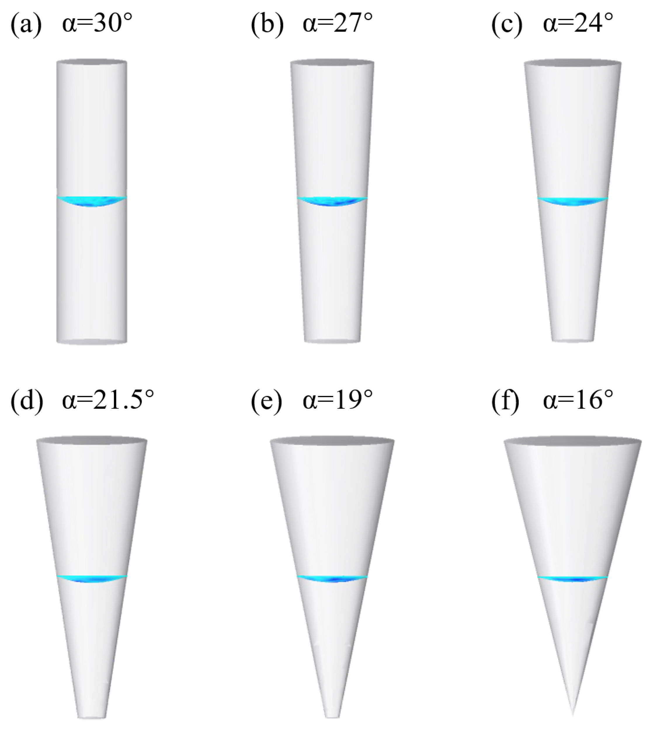
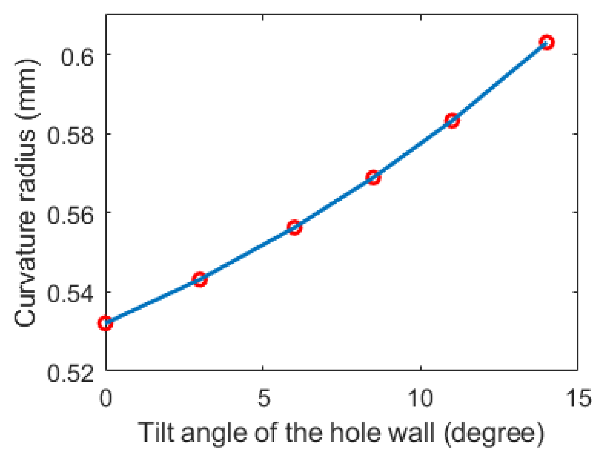
6. Microlenses Based on Microfluidic Flip-Flop Molds with Inclined Wall Holes

In order to achieve controllable microlens curvature, we establish the controlled surface microlens with an inclined hole wall structure [26] for the study. There is a relationship between the inclination angle of the hole wall, the contact angle formed by the photoresist and the microhole wall, and the curvature of the microlens, as shown in Figure 11. By adjusting the inclination angle of the hole wall, we can obtain microlenses with adjustable curvature. The relationship between the inclination angle β of the hole wall, the contact angle θ formed by the photoresist and the microhole wall, and the contact angle α of the microlens is shown in Equation (21). On the basis of the constant contact angle formed by the photoresist and the microhole wall, by adjusting the inclination angle β of the hole wall, we can obtain microlenses with different contact angles α to realize the adjustable curvature. Compared with a rectangular mold, the microlens mold with inclined hole wall structures is able to achieve adjustable curvature without changing the contact angle formed by the photoresist and the microhole wall.
α + θ + β = 90 ° ,
By modeling the rise of the liquid surface in the microholes, we can get the concave liquid surface under different contact angles. The microlenses with different contact angles are finally obtained to realize the adjustable curvature.
For the numerical modeling, following the COMSOL simulation method for cylindrical models, we model the liquid level rise in microholes with inclined hole walls. First, we build a cylinder with a radius of 0.5 mm and a height of 8 mm. The cylinder is divided into two parts: the upper part is air, and the lower part is liquid. Then, we adjust the inclination angle β of the hole wall, which is 0°, 3°, 6°, 8.5°, 11°, and 14°. Keeping the contact angle θ between the photoresist in the microhole and the microhole wall unchanged, the contour of the liquid surface in the microhole with inclined hole wall structure with a contact angle θ of 20° was finally obtained, as shown in Figure 12.
For the theoretical model, through the derivation of the equation, we establish the inclined hole wall cylindrical surface model. The theoretical model is based on the space xyz coordinate system. Through Equation (22), we can obtain the inclined hole wall cylindrical surface model.
z = R 2 x 2 y 2 ,
where R = r cos ( β + θ ) , r is the cylindrical radius, and θ is the contact angle.
By using the formula, we can see the relationship between the inclination angle of the hole wall and the radius of curvature of the microlens surface, as shown in Figure 13.

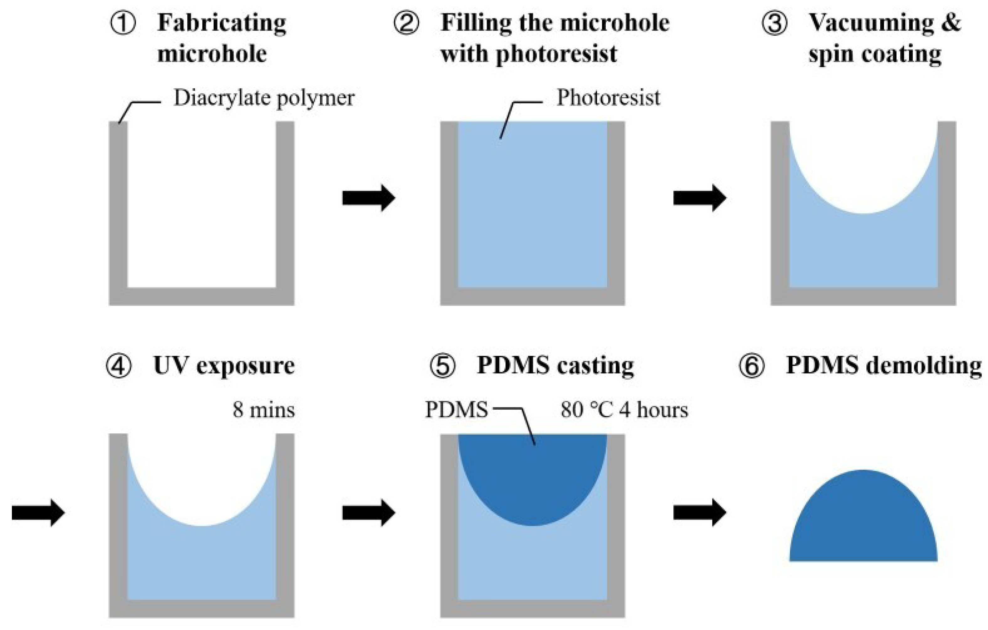
7. Schemes for Microlens Fabrication

The fabrication method of the microlens is briefly described in Figure 14: First, the microholes are fabricated via 3D printing. Photoresist is poured into the microhole. Then, the photoresist-filled microhole is put into a vacuum machine to remove the air bubbles in the microhole. The microhole is spin-coated. After the microhole is stabilized, the photoresist is cured by exposing the microhole to UV light. In this way, the mold for fabricating the microlens can be obtained. Then, polydimethylsiloxane (PDMS) is poured into the pre-fabricated microhole mold and the microhole is filled. The mold is heated. After the PDMS is cured, the PDMS is demolded from the microhole. In this way, the desired microlens can be obtained.

8. Conclusions

In this paper, a theoretical model of curved liquid surface in the microholes for molding microlens is proposed. Round, square, and hexagonal microlenses with adjustable curvature can be obtained by controlling the contact angle between the photoresist in the microhole and the wall of the microhole via capillary force action. This paper provides the theoretical explanation and mathematical model for the formation of the liquid surface in the microholes of different shapes. A numerical model based on the FDTD method is also given for verification. The profiles calculated by the mathematical model match those obtained by the FDTD method. The influence of the shape of the microholes and the contact angles of the liquid in the microholes over the profile of the surface is investigated. Furthermore, 3D models of the microlenses that have replicated profiles of the liquid surfaces are presented. The optical properties of the microlenses in different shapes can be studied. As the contact angle of the microlens gradually increases, both the back focal length and the effective focal length of the microlens gradually decrease. The hexagonal microlens exhibits a great change of back focal length and effective focal length with the variation of the contact angles compared to the round microlens and the square microlens. As for the aberration, the phase difference is small for all three shapes of microlenses. The proposed theoretical model provides an analytical way to study the properties of microlenses, making the microlens and microlens array design simple and straightforward.

Author Contributions

Conceptualization, Y.S. and B.D.; methodology, Y.S. and B.D.; software, Y.S. and Y.L.; validation, Y.S. and B.D.; formal analysis, Y.S. and B.D.; investigation, Y.S. and B.D.; resources, B.D.; data curation, Y.S.; writing—original draft preparation, Y.S.; writing—review and editing, Y.S., Y.L., X.Z., L.W. and B.D.; visualization, Y.S., L.W. and B.D.; supervision, B.D.; project administration, B.D. and D.Z.; funding acquisition, B.D. and D.Z. All authors have read and agreed to the published version of the manuscript.

Funding

This research was supported by the National Natural Science Foundation of China (No. 62205017, 62475157), and Three-Year Public Health Action Plan of Shanghai (No. GWVI-11.1-13).

Data Availability Statement

The study did not report any data. Figures were generated using COMSOL, ZEMAX, and MATLAB.

Conflicts of Interest

The authors declare no conflicts of interest.

References

  1. Han, J.L.; Zhang, J.; Shan, X.N.; Zhang, Y.W.; Peng, H.Y.; Qin, L.; Tan, Y.N.; Wang, L.J. Conversion of a Gaussian-distributed circular beam to a flat-top-distributed square beam in laser shock processing based on a micro-lens array structure. Optik 2023, 274, 170525. [Google Scholar] [CrossRef]
  2. Gradkowski, K.; Morrissey, P.E.; Brien, P. Packaging of micro-lens arrays to photonic integrated circuits using beam shape evaluation. J. Phys. Photonics 2024, 6, 035022. [Google Scholar]
  3. Garza-Rivera, A.; Gómez-Correa, J.E.; Renero-Carrillo, F.J.; Trevino, J.P.; Coello, V. Gabor superlens with variable focus. Chin. Opt. Lett. 2020, 18, 122201. [Google Scholar]
  4. Wang, W.W.; Chen, G.X.; Weng, Y.L.; Weng, X.Y.; Zhou, X.T.; Wu, C.X.; Guo, T.L.; Yan, Q.; Lin, Z.X.; Zhang, Y.G. Large-scale microlens arrays on flexible substrate with improved numerical aperture for curved integral imaging 3D display. Sci. Rep. 2020, 10, 11741. [Google Scholar]
  5. Choi, I.S.; Park, S.; Jeon, S.; Kwon, Y.W.; Park, R.; Taylor, R.A.; Kyhm, K.; Hong, S.W. Strain-tunable optical microlens arrays with deformable wrinkles for spatially coordinated image projection on a security substrate. Microsyst. Nanoeng. 2022, 8, 98. [Google Scholar]
  6. Liu, Z.H.; Hu, G.W.; Ye, H.P.; Wei, M.Y.; Guo, Z.H.; Chen, K.X.; Liu, C.; Tang, B.; Zhou, G.F. Mold-free self-assembled scalable microlens arrays with ultrasmooth surface and record-high resolution. Light Sci. Appl. 2023, 12, 143. [Google Scholar] [CrossRef]
  7. Xu, C.; Guan, X.; Abbasi, S.A.; Xia, N.; Ngai, T.; Zhang, L.; Ho, H.P.; Ng, S.H.C.; Yuan, W. Liquid-shaped microlens for scalable production of ultrahigh-resolution optical coherence tomography microendoscope. Commun. Eng. 2024, 3, 1. [Google Scholar] [CrossRef]
  8. Ahn, K.H.; Park, E.S.; Nam, S.M. Usefulness of a 1064 nm Microlens Array-type, Picosecond-dominant Laser for Pigmented Scars with Improvement of Vancouver Scar Scale. Med. Lasers 2019, 8, 19. [Google Scholar]
  9. Choi, J.; Duc, T.M.; Kim, H.; Hwang, J.K.; Kang, H.W. Diffractive micro-lens array (DLA) for uniform and selective picosecond laser treatment. Biomed. Opt. Express 2023, 14, 1992. [Google Scholar]
  10. Liang, X.X.; Yan, M.M.; Xu, Y.Z.; Zhang, T.C.; Zhang, D.N.; Zhang, C.R.; Wang, B.; Yi, F.T.; Liu, J. The fabrication of microlens array in PMMA material with the assistant of nickel pillars by LIGA technology and thermal reflow method. Microsyst. Technol. 2023, 29, 763. [Google Scholar]
  11. Yong, Y.Q.; Chen, S.; Chen, H.; Ge, H.X.; Hao, Z.B. A Rapid Fabrication Method of Large-Area MLAs with Variable Curvature for Retroreflectors Based on Thermal Reflow. Micromachines 2024, 15, 816. [Google Scholar] [CrossRef] [PubMed]
  12. Wu, Y.; Dong, X.S.; Wang, X.F.; Xiao, J.F.; Sun, Q.Q.; Shen, L.F.; Lan, J.; Shen, Z.F.; Xu, J.F.; Du, Y.Q.Y. Fabrication of Large-Area Silicon Spherical Microlens Arrays by Thermal Reflow and ICP Etching. Micromachines 2024, 15, 460. [Google Scholar] [CrossRef] [PubMed]
  13. Wang, Z.H.; Wu, Y.L.; Chen, L.; Bakhtiyari, A.N.; Yu, W.H.; Qi, D.F.; Zheng, H.Y. Spatial light assisted femtosecond laser direct writing of a bionic superhydrophobic Fresnel microlens arrays. Opt. Laser Technol. 2024, 180, 111451. [Google Scholar]
  14. Deng, H.T.; Qi, D.F.; Wang, X.M.; Liu, Y.H.; Shangguan, S.Y.; Zhang, J.G.; Shen, X.; Liu, X.Y.; Wang, J.; Zheng, H.Y. Femtosecond laser writing of infrared microlens arrays on chalcogenide glass. Opt. Laser Technol. 2023, 159, 108953. [Google Scholar]
  15. Huang, L.; Hong, Z.H.; Chen, Q.D.; Zhang, Y.L.; Zhao, S.Q.; Dong, Y.J.; Liu, Y.Q.; Liu, H. Imaging/nonimaging microoptical elements and stereoscopic systems based on femtosecond laser direct writing. Light Adv. Manuf. 2023, 4, 543. [Google Scholar]
  16. Wang, H.; Zhang, W.; Ladika, D.; Yu, H.; Gailevičius, D.; Wang, H.; Pan, C.; Nair, P.N.S.; Ke, Y.; Mori, T.; et al. Two-Photon Polymerization Lithography for Optics and Photonics: Fundamentals, Materials, Technologies, and Applications. Adv. Funct. Mater. 2023, 33, 2214211. [Google Scholar]
  17. Wang, Z.H.; Wu, Y.L.; Yu, W.H.; Qi, D.F.; Bakhtiyari, A.N.; Zheng, H.Y. Investigation into fabrication and optical characteristics of tunable optofluidic microlenses using two-photon polymerization. Opt. Express 2024, 32, 7448. [Google Scholar]
  18. Dirdal, C.A.; Jensen, G.U.; Angelskår, H.; Thrane, P.C.V.; Gjessing, J.; Ordnung, D.A. Towards high-throughput large-area metalens fabrication using UV-nanoimprint lithography and Bosch deep reactive ion etching. Opt. Express 2020, 28, 15542. [Google Scholar]
  19. Zheng, J.X.; Tian, K.S.; Qi, J.Y.; Guo, M.R.; Liu, X.Q. Advances in fabrication of micro-optical components by femtosecond laser with etching technology. Opt. Laser Technol. 2023, 167, 109793. [Google Scholar]
  20. Aderneuer, T.; Fernández, O.; Ferrini, R. Two-photon grayscale lithography for free-form micro-optical arrays. Opt. Express 2021, 29, 39511. [Google Scholar]
  21. Lamprecht, B.; Ulm, A.; Lichtenegger, P.; Leiner, C.; Nemitz, W.; Sommer, C. Origination of free-form micro-optical elements using one- and two-photon grayscale laser lithography. Appl. Opt. 2022, 61, 1863. [Google Scholar] [CrossRef] [PubMed]
  22. Garcia, I.S.; Ferreira, C.; Santos, J.D.; Martins, M.; Dias, R.A.; Aguiam, D.E. Fabrication of a MEMS Micromirror Based on Bulk Silicon Micromachining Combined with Grayscale Lithography. J. Microelectromech. Syst. 2020, 29, 734. [Google Scholar] [CrossRef]
  23. Chen, P.C.; Chang, Y.P.; Zhang, R.H.; Wu, C.C.; Tang, G.R. Microfabricated microfluidic platforms for creating microlens array. Opt. Express 2017, 25, 16101. [Google Scholar] [CrossRef] [PubMed]
  24. Xu, Q.; Dai, B.; Huang, Y.; Wang, H.; Yang, Z.; Wang, K.; Zhuang, S.; Zhang, D.W. Fabrication of polymer microlens array with controllable focal length by modifying surface wettability. Opt. Express 2018, 26, 4172. [Google Scholar] [CrossRef]
  25. Liu, C.; Wang, D.; Wang, Q.; Xing, Y. Multifunctional optofluidic lens with beam steering. Opt. Express 2020, 28, 7734. [Google Scholar] [CrossRef]
  26. Long, Y.; Song, Z.Y.; Pan, M.L.; Tao, C.X.; Hong, R.J.; Dai, B.; Zhang, D.W. Fabrication of uniform-aperture multi-focus microlens array by curving microfluid in the microholes with inclined walls. Opt. Express 2021, 29, 12763. [Google Scholar] [CrossRef]
  27. Bogdanowicz, R.; Jönsson-Niedziółka, M.; Vereshchagina, E.; Dettlaff, A.; Boonkaew, S.; Pierpaoli, M.; Wittendorp, P.; Jain, S.; Tyholdt, F.; Thomas, J.; et al. Microfluidic devices for photo-and spectroelectrochemical applications. Curr. Opin. Electrochem. 2022, 36, 101138. [Google Scholar] [CrossRef]
  28. Golozar, M.; Chu, W.K.; Casto, L.D.; McCauley, J.; Butterworth, A.L.; Mathies, R.A. Fabrication of high-quality glass microfluidic devices for bioanalytical and space flight applications. MethodsX 2020, 7, 101043. [Google Scholar] [CrossRef]
  29. Dai, B.; Zhang, L.; Zhao, C.L.; Bachman, H.; Becker, R.; Mai, J.; Jiao, Z.; Li, W.; Zheng, L.L.; Wan, X.J.; et al. Biomimetic apposition compound eye fabricated using microfluidic-assisted 3D printing. Nat. Commun. 2021, 12, 6458. [Google Scholar] [CrossRef]
  30. Xu, Z.H.; Zhou, J.Y.; Wang, B.; Meng, Z.M. Design of Refractive/Diffractive Hybrid Projection Lens for DMD-Based Maskless Lithography. Optics 2021, 2, 103–112. [Google Scholar] [CrossRef]
  31. Xu, M.; Li, J.; Chang, X.Y.; Chen, C.F.; Lu, H.B.; Wang, Z. Self-assembled microlens array with controllable curvatures for integral imaging 3D display. Opt. Lasers Eng. 2024, 180, 108322. [Google Scholar] [CrossRef]
  32. Gerlach, F.; Hussong, J.; Roisman, I.V.; Tropea, C. Capillary rivulet rise in real-world corners. Colloids Surf. A Physicochem. Eng. Asp. 2020, 592, 124530. [Google Scholar] [CrossRef]
  33. Li, C.X.; Dai, H.Y.; Gao, C.; Jiang, L. Bioinspired inner microstructured tube controlled capillary rise. Appl. Biol. Sci. 2019, 116, 12704. [Google Scholar] [CrossRef]
  34. Zuo, Z.W.; Wang, J.F.; Huo, Y.P.; Wang, D.B.; Ji, H.B. Experimental simulation of capillary effect on rough flat surfaces. Particuology 2022, 60, 115. [Google Scholar] [CrossRef]
  35. Abadi, G.B.; Bahrami, M. The effect of surface roughness on capillary rise in micro-grooves. Sci. Rep. 2022, 12, 14867. [Google Scholar]
  36. Chen, S.T.; Duan, L.; Li, Y.; Ding, F.L.; Liu, J.T.; Li, W. Capillary Phenomena Between Plates from Statics to Dynamics Under Microgravity. Microgravity Sci. Technol. 2022, 34, 70. [Google Scholar]
  37. Li, W.; Wu, D.; Li, Y.; Chen, S.Y.; Ding, F.L.; Kang, Q.; Chen, S.T. Static profiles of capillary surfaces in the annular space between two coaxial cones under microgravity. Acta Mech. Sin. 2024, 40, 123218. [Google Scholar]
  38. Son, S.Y.; Chen, L.; Kang, Q.J.; Derome, D.; Carmeliet, J. Contact Angle Effects on Pore and Corner Arc Menisci in Polygonal Capillary Tubes Studied with the Pseudopotential Multiphase Lattice Boltzmann Model. Computation 2016, 4, 12. [Google Scholar] [CrossRef]
  39. Mohseni, K. Surface Tension Capillarity and Contact Angle. In Encyclopedia of Microfluidics and Nanofluidics; Li, D., Ed.; Springer: Boston, MA, USA, 2008; pp. 1949–1956. [Google Scholar]
  40. Liou, W.W.; Peng, Y.Q.; Parker, P.E. Analytical modeling of capillary flow in tubes of nonuniform cross section. J. Colloid Interface Sci. 2009, 333, 389–399. [Google Scholar] [CrossRef]
  41. Vermolen, F.; Gharasoo, M.G.; Zitha, P.L.J.; Bruining, J. Numerical Solutions of Some Diffuse Interface Problems: The Cahn-Hilliard Equation and the Model of Thomas and Windle. Int. J. Multiscale Comput. Eng. 2009, 7, 523–543. [Google Scholar] [CrossRef]
  42. Athukorallage, B.; Iyer, R. On a two-point boundary value problem for the 2-D Navier-Stokes equations arising from capillary effect. Math. Model. Nat. Phenom. 2020, 15, 17. [Google Scholar]
  43. Wu, P.K.; Zhang, H.; Nikolov, A.; Wasan, D. Rise of the main meniscus in rectangular capillaries: Experiments and modeling. J. Colloid Interface Sci. 2016, 461, 195. [Google Scholar] [PubMed]
  44. Durán-Ramírez, V.M.; Muñoz-Maciel, J.; Casillas-Rodríguez, F.J.; Mora-Gonzalez, M.; Peña-Lecona, F.G. Exact Equations for the Back and Effective Focal Lengths of a Plano-Concave Thick Lens. Optics 2024, 5, 452–464. [Google Scholar] [CrossRef]
Figure 1. (a) The model of the microlens mold. (b) The demolded microlens.
Optics 06 00013 g001
Figure 2. The profile of the liquid surface in the cylindrical microholes with α of 10°, 20°, 30°, and 40°, respectively.
Optics 06 00013 g002
Figure 3. The profile of the liquid surface in the square microholes with α of 10°, 20°, 30°, and 40°, respectively.
Optics 06 00013 g003
Figure 4. The profile of the liquid surface in the hexagonal microholes with α of 10°, 20°, 30°, and 40°, respectively.
Optics 06 00013 g004
Figure 5. Schematic diagram of the lower concave liquid level, g r e e n   l i n e = r cos ( θ ) , y e l l o w   l i n e = r tan ( θ ) , h = r cos ( θ ) r tan ( θ ) .
Optics 06 00013 g005
Figure 6. The surface profiles in the (a) cylindrical, (b) square, and (c) hexagonal microholes calcu-lated by the FDTD model. The surface profiles in the (d) cylindrical, (e) square, and (f) hexagonal microholes calculated by the proposed mathematical model. The deviation between the results ob-tained by the two models for the surface profiles in the (g) cylindrical, (h) square, and (i) hexagonal microholes, respectively.
Optics 06 00013 g006
Figure 7. The microlenses demolded from the molds with radius of 1 mm and α of 10°, 20°, 30°, and 40°, respectively. (a) The round microlenses. (b) The square microlenses. (c) The hexagonal microlenses.
Optics 06 00013 g007
Figure 8. Back focal length and effective focal length of the microlenses. (a) The round microlenses. (b) The square microlenses. (c) The hexagonal microlenses.
Optics 06 00013 g008
Figure 9. The spherical aberration along y-axis and the spherical aberration along x-axis of the mi-crolenses. (a) The round microlenses. (b) The square microlenses. (c) The hexagonal microlenses.
Optics 06 00013 g009
Figure 10. The sectional view of the microlens and the ideal lens with same EFL and pupil diameter.
Optics 06 00013 g010
Figure 11. (ac) Modeling of controlled surface microlens molds with inclined hole wall structures. (df) Modeling of demolded microlenses.
Optics 06 00013 g011
Figure 12. Contours of the liquid surface in microholes with inclined hole wall structure with contact angle θ of 20°.
Optics 06 00013 g012
Figure 13. Relationship between the inclination angle of the hole wall and the radius of curvature of the microlens surface.
Optics 06 00013 g013
Figure 14. The fabrication procedure of the microlens.
Optics 06 00013 g014
Disclaimer/Publisher’s Note: The statements, opinions and data contained in all publications are solely those of the individual author(s) and contributor(s) and not of MDPI and/or the editor(s). MDPI and/or the editor(s) disclaim responsibility for any injury to people or property resulting from any ideas, methods, instructions or products referred to in the content.

