Electronic Population Reconstruction from Strong-Field-Modified Absorption Spectra with a Convolutional Neural Network

Abstract

We simulate ultrafast electronic transitions in an atom and corresponding absorption line changes with a numerical, few-level model, similar to previous work. In addition, a convolutional neural network (CNN) is employed for the first time to predict electronic state populations based on the simulated modifications of the absorption lines. We utilize a two-level and four-level system, as well as a variety of laser-pulse peak intensities and detunings, to account for different common scenarios of light–matter interaction. As a first step towards the use of CNNs for experimental absorption data in the future, we apply two different noise levels to the simulated input absorption data.

1. Introduction

The development of attosecond laser sources [1,2,3] not only allows for capturing electronic motion in atoms, molecules and solids on their natural time scales, but it has also expanded the spectral regime of ultrafast pulses into the ultraviolet (UV) and extreme-ultraviolet (XUV) ranges. Besides the pioneering work on high-order harmonic generation (HHG) from near-infrared optical pulses [1,2,3], free-electron lasers can also generate XUV laser pulses [4], which are, since recently, also available with attosecond pulse durations [5,6]. One of the crucial benefits of FEL pulses is their high peak intensity, which allows for all-XUV pump–probe experiments [7] and strong-field effects in the XUV range on ultrashort time scales, such as Rabi cycling [8] or absorption line shape modifications [9,10,11,12]. Although properties such as the temporal dipole moment can be reconstructed under certain circumstances [13], the (intra-pulse) time-dependent state populations have not yet been directly reconstructed. This kind of inversion problem is common in a broad variety of quantum-based experiments, where phase information is typically lost and inversions are non-trivial, if possible at all. Still, electronic state populations and coherences are crucial for understanding effects such as Rabi cycling [8] or X-ray lasing [14] in atoms or charge transfer in molecules [15,16,17].

In contrast, machine learning (ML) in general and especially neural networks [18] as a subtype of ML based on multilayers of interconnected ‘neurons’ are well-known methods for pattern recognition and solving inversion problems. While nowadays utilized in broad areas and diverse applications, ML has recently also been used in ultrafast science, for example, in laser pulse reconstructions [19,20,21,22,23,24], high-order harmonic generation [25], noise reduction [26] and molecular- [27,28,29,30] or electronic-structure reconstruction methods [31,32,33]. In these applications, neural networks [19,20,21,22,23,25,27,28,30,33], and especially convolutional neural networks (CNNs) [23,27,28,30,33], based on convolutional operations on spectral data, are utilized frequently. A common technique is to train the CNNs on simulated or modeled datasets [21,23,24,25,27,28,30,33] and (potentially) use them on experimental data afterwards. Besides large-scale quantum simulations and experimental approaches, ML can provide new insights for data analysis and reconstruction problems, with the goal of ultimately enhancing the understanding of the underlying quantum processes. Most recently, the first steps towards reconstructing time-resolved molecular dynamics have been demonstrated [28].

In this work, we simulate strong-field-induced line shape modifications with a numerical, few-level system, similar to previous work [9,10,11,12]. Furthermore, we implement a CNN, which reconstructs the electronic populations during the driving pulse from the simulated strong-field-modified absorption spectra of a two-level system. To allow the CNN to predict populations from experimental data in the future, we also introduce different noise levels into the absorption spectra before training the CNN. To extend our model towards more complex electron dynamics involving several states, we additionally apply the CNN to a four-level system, where a coherent wavepacket of three excited states is initiated.

2. Materials and Methods

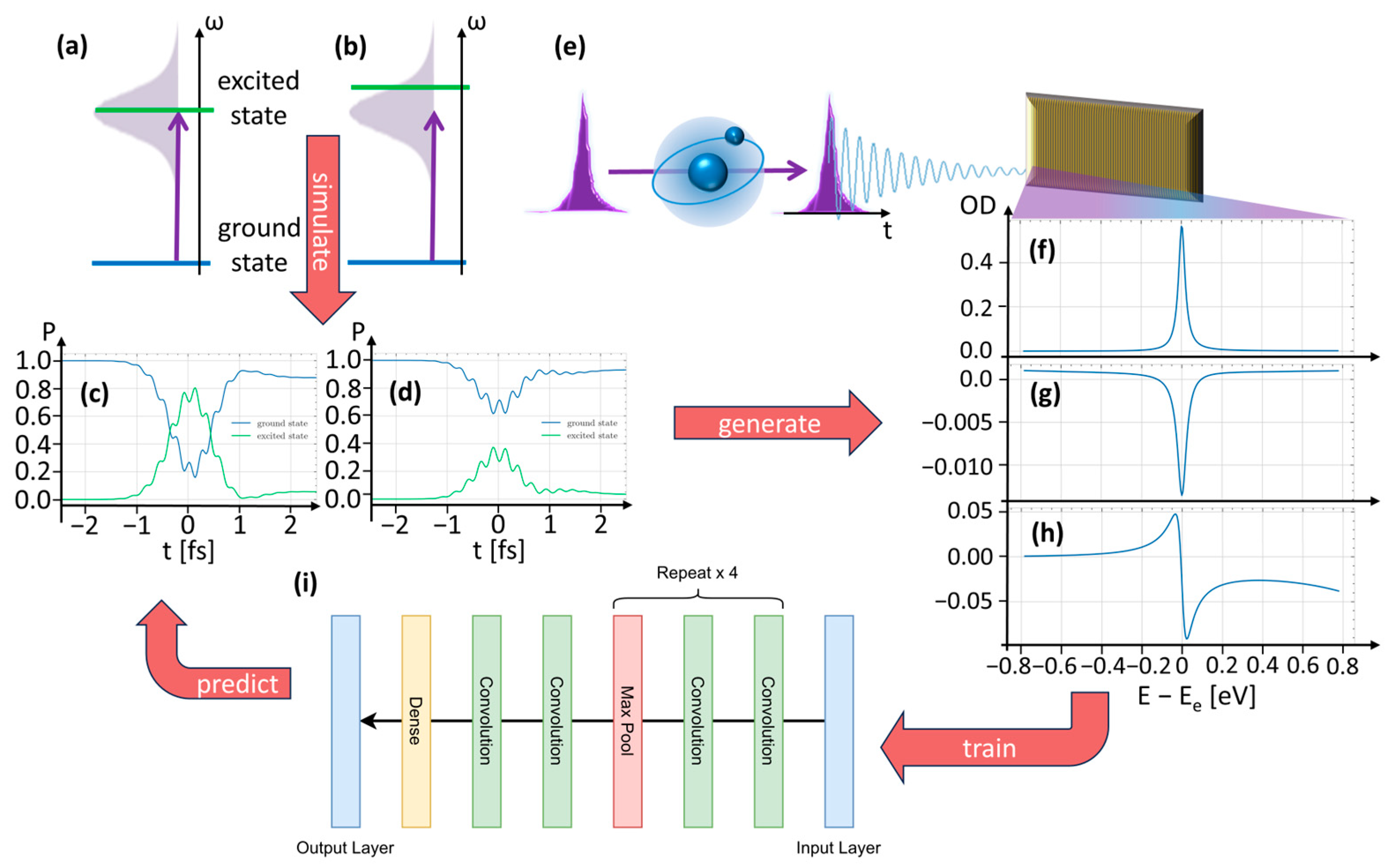
2.1. Few-Level Systems for Simulations of Absorption Line Shape Changes

To simulate strong-field light–matter interaction and the resulting absorption changes, we consider a few-level system and solve the Schrödinger equation numerically, as described in detail in our previous work [11]. First, we describe a generic two-electronic-state system in an atom interacting with a laser pulse, cf. Figure 1a,b, with a Hamiltonian as follows:

$${\mathrm{H}}_{2\mathrm{l}\mathrm{v}\mathrm{l}}=\left(\begin{array}{cc}{\mathrm{E}}_{\mathrm{g}}& {\mathrm{d}}_{\mathrm{g}\mathrm{e}}\mathsf{\epsilon }\left(\mathrm{t}\right)\\ {\mathrm{d}}_{\mathrm{g}\mathrm{e}}\mathsf{\epsilon }\left(\mathrm{t}\right)& {\mathrm{E}}_{\mathrm{e}}-\mathrm{i}\mathrm{h}{\mathsf{\Gamma }}_{\mathrm{e}}/2\end{array}\right)$$

(1)

The diagonal matrix elements contain the eigenstate energies of the ground (g) and excited (e) state, E_g = 0 a.u and E_e = 0.2932 a.u., and the inverse lifetime of the excited state, ${\mathsf{\Gamma }}_{\mathrm{e}}$ = 0.002 a.u. (a.u. denotes atomic units). The i represents the imaginary unit, whereas the h is the Planck constant. The off-diagonal matrix elements describe the dipole coupling between the two states, where we choose d_ge = d_eg = 1 a.u. as the dipole constant and ε(t) is the electric field of the laser pulse. We use a Gaussian pulse defined in the spectral domain $\tilde{\mathsf{\epsilon }}(\omega )$, with a spectral width of σ = 0.02314 a.u., corresponding to a 2.5 fs pulse duration, and centered at the resonance transition of the two states. To additionally produce a detuned dataset, we shift the excited-state energy by 0.0568 a.u towards lower photon energies without changing the laser pulse parameters. The time-dependent Schrödinger equation is solved for each time step t between −2.5 fs and 2.5 fs relative to the pulse peak intensity in steps of 0.025 fs. The two resulting time-dependent populations, P_g,e(t) = |c_g,e(t)|², of the bare states are shown in Figure 1c,d for the resonant and detuned pulses, respectively. c_g,e are the coefficients of the general quantum state of the system, $\left|\mathsf{\Psi }\right(\mathrm{t})⟩={\left[{\mathrm{c}}_{\mathrm{g}}\right(\mathrm{t}),{\mathrm{c}}_{\mathrm{e}}(\mathrm{t}\left)\right]}^{\mathrm{T}}$, in the basis of the two bare states. With the help of the state coefficients, we can calculate the dipole response of the two-level system, d(t) = d_ge$·$c_g(t)c_e × (t) + c.c., see Figure 1e, and its Fourier transform, $\tilde{\mathrm{d}}(\mathsf{\omega })$. In the case of strong coupling dynamics, the resulting energy-level shifts lead to a phase shift of the temporal dipole response since the laser pulse is (much) shorter than the lifetime of the excited state [34]. This leads to line shape changes in the optical density, $\mathrm{O}\mathrm{D}\left(\mathsf{\omega }\right)$, which we calculate from the in- and outgoing fields:

$$\mathrm{O}\mathrm{D}\left(\mathsf{\omega }\right)=-{\mathrm{l}\mathrm{o}\mathrm{g}}_{10}\left(\frac{{\left|\tilde{\mathsf{\epsilon }}\left(\mathsf{\omega }\right)+\mathrm{i}\mathsf{\eta }·\tilde{\mathrm{d}}\left(\mathsf{\omega }\right)\right|}^2}{{\left|\tilde{\mathsf{\epsilon }}\left(\mathsf{\omega }\right)\right|}^2}\right)$$

(2)

Here, $\mathsf{\eta }={10}^{-4}$ is a numerical constant, proportional to the particle density in an absorption experiment. We illustrate the change in the resonance line shape in $\mathrm{O}\mathrm{D}\left(\mathsf{\omega }\right)$ from the weak-field case in Figure 1f to the strongly driven case for resonant and detuned pulses, shown in Figure 1g,h, respectively. $\mathrm{O}\mathrm{D}\left(\mathsf{\omega }\right)$ is the input for the CNN, see Figure 1i, which is used to reconstruct the populations, as described in the next section.

Regarding the four-level system, we replace the Hamiltonian with a 4 × 4 matrix containing the four eigen-energies of the ground state and the three excited states (e1, e2 e3): E_g = 0 a.u, E_e1 = 0.2676 a.u., E_e2 = 0.2932 a.u. and E_e3 = 0.315 a.u. For all three excited states, we use the same inverse lifetime and dipole constant as for the two-level system. No dipole couplings are allowed between any two excited states by setting all other off-diagonal matrix elements to zero. The laser pulse is defined as above and resonant with the second excited state, thus also being equally red- and blue-detuned as the two other excited states.

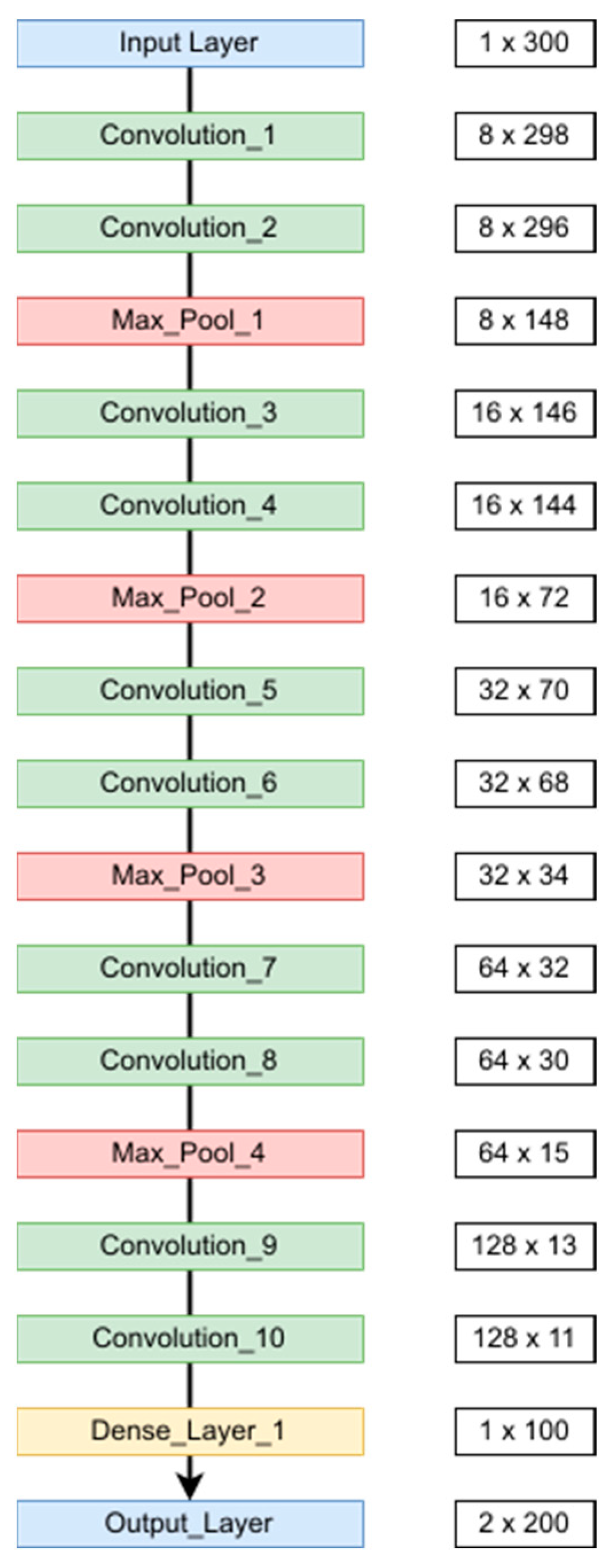
2.2. Convolutional Neutral Network for State Population Reconstruction

2.2.1. Convolutional Neural Network Architecture

The inputs for the CNN are the OD spectra sampled with 300 data points symmetrically around the resonance position. The output variables of the CNN are the electron populations, each sampled on a time grid centered around a pulse between −2.5 fs and 2.5 fs with 200 points. For the two-level system, this results in a prediction of 2 × 200 output variables based on 300 input variables. To achieve such a high-dimensional output (relative to the input), the CNN architecture is constructed with several layers, in total containing 279,932 trainable parameters. The CNN layer-by-layer structure, which is constructed in a similar way as the methodologies in [30,33] describe, is depicted in Figure 2. The CNN architecture is characterized by five blocks, each comprising two convolutional layers with a convolution window of size = 3 (kernel) and stride = 1, which is the step size by which the convolutional window moves across the input data. After each convolutional operation within the network, the convolutional layers are followed up by the Rectified Linear Unit (ReLU) activation function, defined as ReLU(x) = max(0, x). The convolutional operations are calculated without padding, resulting in an array size shrinkage of 2 after each layer. In each block, the two convolutional layers are followed up by a max-pooling layer with a kernel size = 2 and stride = 2. The inclusion of max-pooling layers segments the arrays into pooling regions of size 2, resulting in a further reduction in array dimensions by half after each block. To allow for more complex patterns to be captured by the CNN, the number of filters in each convolutional layer is doubled between consecutive blocks, ranging from 8 filters in the initial block to 128 filters in the last block. For the final block, the max-pooling layer is replaced by a densely, i.e., fully connected layer (with ReLU activation) consisting of 100 neurons. The final output layer is also a dense layer (with linear activation) with an output size of 2 × 200—quantifying the two time-dependent populations of the two-level system.

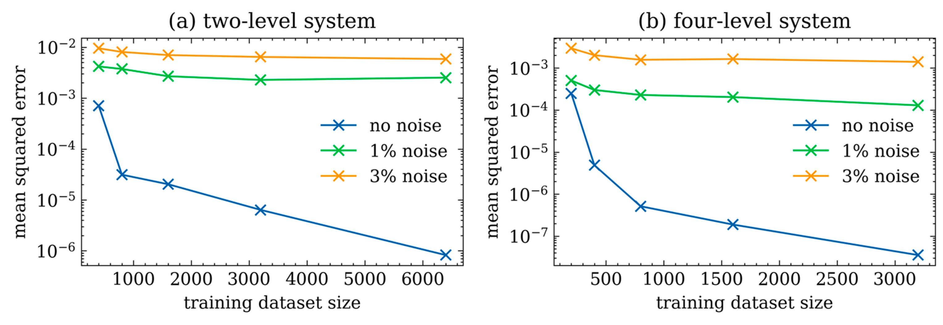
2.2.2. Training Dataset Properties

For the training phase, we generated a comprehensive dataset consisting of 10,000 samples through repeated simulations of the two-level model by randomly sampling the peak field strength of the driving laser pulse, ε₀, on a logarithmic scale, ranging from 0.1 a.u. to 10 a.u. The random sampling improves consistency, promotes comparability and serves to minimize randomness as a confounding factor during the training process. This dataset combines the resonant and detuned cases introduced in Section 2.1. We allocate subsets of 6400 of these samples for training, 1600 for validation during training and 2000 for subsequent testing. Exactly one half of all (sub)sets are calculated with the resonant and detuned settings, respectively. Furthermore, we generate two more datasets by introducing two Gaussian noise levels into the OD spectra. The two noise levels, 1% and 3%, are given as the standard deviation of Gaussian sampled noise. We chose these noise levels based on our experimental observations, for example, detecting absorption changes at a 2% level clearly above a smaller noise level in [35]. For the four-level system, as described in Section 2.1, we use nearly the same architecture as for the two-level system. Since the output variables, i.e., the state populations, are twice as large as before, 4 × 200, we also increase the resolution of the OD to 350 points to maintain comparable predictive resolution. This results in a total network size of 358,732 trainable parameters for the four-level system.

2.2.3. Training Process

To train the CNN, we utilize the Adam optimizer [36], a widely known optimization algorithm used for training deep neural networks. Both the selection of the optimizer and an initial learning rate of 10⁻³ are grounded in a heuristic approach, given that the Adam optimizer inherently adapts the learning rate during training. For the established regression task, the mean-squared error (MSE) is used as the loss function. This metric quantifies the average squared difference between predicted and actual values, thereby providing a measure of the CNN’s proficiency in capturing the deviations between simulated and reconstructed populations.

$$\mathrm{M}\mathrm{S}\mathrm{E}\left(\mathrm{y},\widehat{\mathrm{y}}\right)=\frac{1}{{\mathrm{n}}_{\mathrm{s}\mathrm{a}\mathrm{m}\mathrm{p}\mathrm{l}\mathrm{e}\mathrm{s}}}\sum _{\mathrm{i}=1}^{{\mathrm{n}}_{\mathrm{s}\mathrm{a}\mathrm{m}\mathrm{p}\mathrm{l}\mathrm{e}\mathrm{s}}}{\left({\mathrm{y}}_{\mathrm{i}}-\widehat{{\mathrm{y}}_{\mathrm{i}}}\right)}^2$$

(3)

Here, $\widehat{{\mathrm{y}}_{\mathrm{i}}}$ are the (simulated) input values and y_i are the values predicted by the CNN. The sample size, ${\mathrm{n}}_{\mathrm{s}\mathrm{a}\mathrm{m}\mathrm{p}\mathrm{l}\mathrm{e}\mathrm{s}},$ sums over all data points, including all populations, time steps and laser field strengths. By training the CNN on datasets of different sizes and quantifying the losses with the MSE, as shown in Figure 3a, we observe the loss to be converged for the scenarios with 1% and 3% noise when our utilized training size of 6400 is reached. The loss function for the set without noise still decreases within the reported number of samples, as expected for a noise-free scenario, since the machine precision was not reached. Our goal is a CNN which, ultimately, can predict populations from (noisy) experimental data; thus, we did not increase the data size for the noise-free scenario. Further, we also use the Mean Absolute Error (MAE) as an additional metric, given as follows:

$$\mathrm{M}\mathrm{A}\mathrm{E}\left(\mathrm{y},\widehat{\mathrm{y}}\right)=\frac{1}{{\mathrm{n}}_{\mathrm{s}\mathrm{a}\mathrm{m}\mathrm{p}\mathrm{l}\mathrm{e}\mathrm{s}}}\sum _{\mathrm{i}=1}^{{\mathrm{n}}_{\mathrm{s}\mathrm{a}\mathrm{m}\mathrm{p}\mathrm{l}\mathrm{e}\mathrm{s}}}\left|{\mathrm{y}}_{\mathrm{i}}-\widehat{{\mathrm{y}}_{\mathrm{i}}}\right|$$

(4)

This choice is grounded in the constraint of our model outputs within the range of zero to one for the populations. Consequently, interpreting the Mean Absolute Error allows for an intuitive understanding of our CNN’s performance because it quantifies the average error over all data points, which can also be read as a percentage, i.e., MAE = 0.01 can be read as an average error of 1% over all data points. We train the two- and four-level CNNs for 5000 epochs each, with early stopping after 1000 epochs if the loss function has already converged. For each epoch, we randomly divide the training set into 100 batches of size 64, on which the CNN is trained iteratively to circumvent the expansive full training dataset size of 6400. After training, only the best-performing model is saved and selected for subsequent testing. As for the two-level case, we evaluate our model with the MSE for different training data sizes, as shown in Figure 3b. For the two cases containing noise, the loss converges for our data size of 3200, whereas the noise-free case has not reached convergence yet.

3. Results

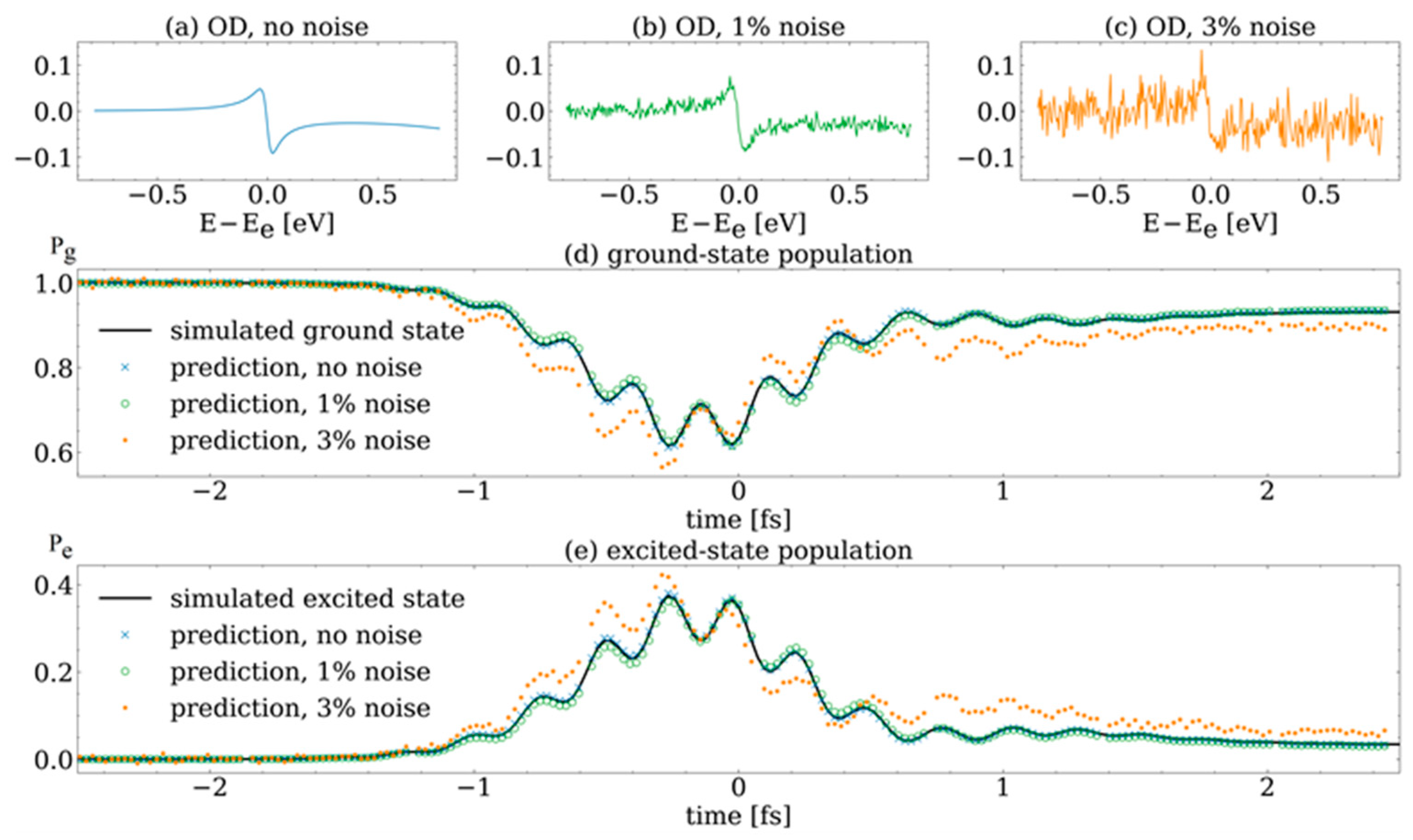
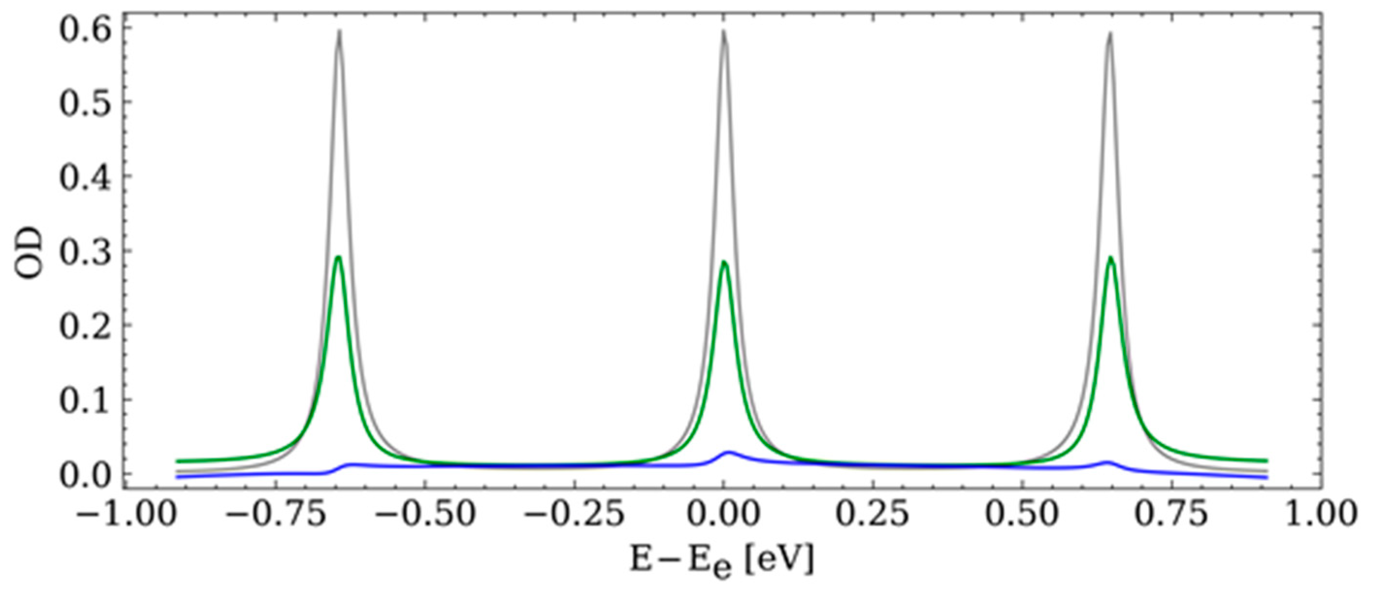
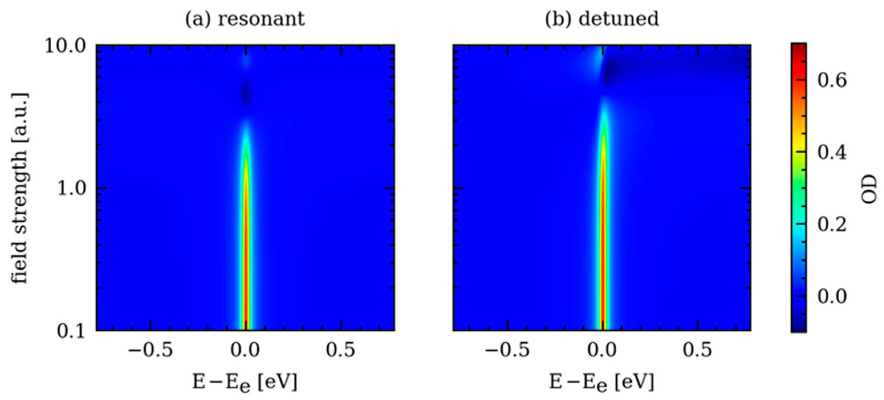
3.1. Line Shape Changes and Population Reconstruction for the Two-Level System

In this section, we first show the results of the simulated absorption spectra (Figure 4) and discuss them with respect to previous findings [11,12]. Afterwards, the results of our novel approach to reconst the time-dependent electronic state populations from the absorption spectra are presented and discussed (Figure 5 and Figure 6). In Figure 4a, the field-strength-dependent absorption is changing continuously in amplitude while staying Lorentzian, thus symmetric. As shown in our previous work [11,12], dipole phase shifts cancel out for exactly resonant driving pulses, hence explaining the symmetric line shape. For electric field strengths of 3.3 a.u. and 6.3 a.u., the resonant OD switches sign due to π-phase jumps in the Rabi cycle of the population coefficients [12]. In contrast, the detuned pulses can change the asymmetry of the resonance line by inducing dipole phase shifts [11,12], as shown in Figure 4b, hence making it Fano-like shaped [37]. For electric field strengths around 5 a.u. to 6 a.u., Fano-like line shapes emerge, which exhibit negative OD. A more detailed discussion of these line shape changes and how they are connected to the electronic state energies and coefficients can be found in [11,12].

In Figure 5, we illustrate that the CNN is capable of reconstructing the populations of the ground (Figure 5d) and excited states (Figure 5e), including the three different noise levels, for a single field strength of ε₀ = 6.1 a.u. of a detuned driving pulse. The OD spectrum is shown in Figure 5a without noise, with a 1% noise level in Figure 5b and a 3% noise level in Figure 5c. For both states—the ground state in Figure 5d and the excited state in Figure 5e—the reconstructed populations for the noise-free case (blue) are in near-perfect agreement with the simulated populations (black). Even when introducing 1% noise into the OD, the CNN reconstructs the state populations excellently (shown in green). In contrast, when the noise level is increased to 3%, only the slow overall shapes of the reconstructed populations (orange) can be predicted reasonably well, whereas the faster dynamics are not accurate anymore. To prove that the CNN can reconstruct the electronic populations in general for the complete dataset, we compare the simulated population (Figure 5a,b) of the excited state to the reconstructed population (Figure 5c,d) as a function of the field strength of the driving pulse in Figure 6. We look at the excited state population only because the sum of the ground state and excited state populations is equal to one for all time steps without the presence of further loss channels. For the CNN reconstruction, we chose the 1% noise level in the OD based on the results obtained for a single electric field strength, as discussed in Figure 5. For the resonant driving pulse, the population is reconstructed excellently for most field strengths in Figure 6c compared to the simulated population in Figure 6a. Only for field strengths from 6.1 a.u. to 6.6 a.u. does the reconstruction differ from the simulation, as discussed below. In the detuned case, the population is reconstructed accurately for most field strengths in Figure 6d compared to Figure 6b. For field strengths of 4.5 a.u. to 4.6 a.u., the reconstruction is significantly different from the simulation. Looking at the corresponding input ODs in Figure 4a,b reveals that for a field strength of 3.3 a.u. and 6.5 a.u. in the resonant case (a) and 4.5 a.u. in the detuned case (b), the ODs are near flat and close to zero. Due to this ambiguity, the CNN cannot distinguish between the three cases where the OD vanishes, which is why the training and reconstruction with the CNN fail in these specific cases.

For a quantitative comparison of the reconstructed with the simulated populations, the MSEs (Equation (3)) and MAEs (Equation (4)) are presented in

Table 1. MSE and MAE of the population reconstruction for the two-level system.

Error	No Noise	1% Noise	3% Noise
MSE	5.7 × 10−7	3.4 × 10−3	5.5 × 10−3
MAE	4.1 × 10−4	1.5 × 10−2	3.3 × 10−2

for all three noise levels. As expected from the above findings, the errors increase with the noise. All error values are a few percent or less, thus confirming the excellent agreement between the reconstructed and simulated populations for most field strengths, with the exceptions mentioned above. This demonstrates that the CNN is capable of reconstructing the populations of two electronic states based on absorption line changes in all cases where the absorption signal is larger than the noise.

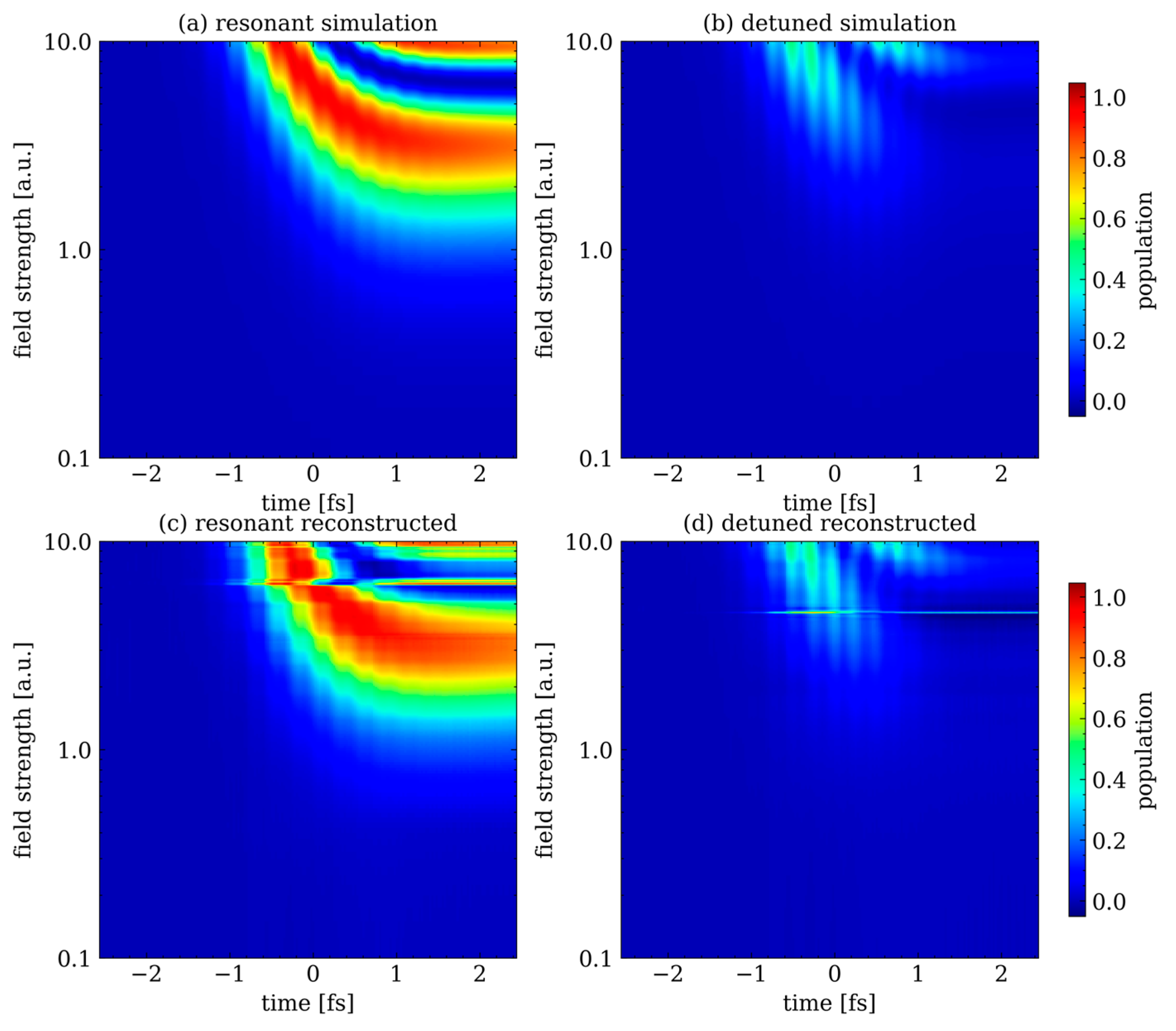
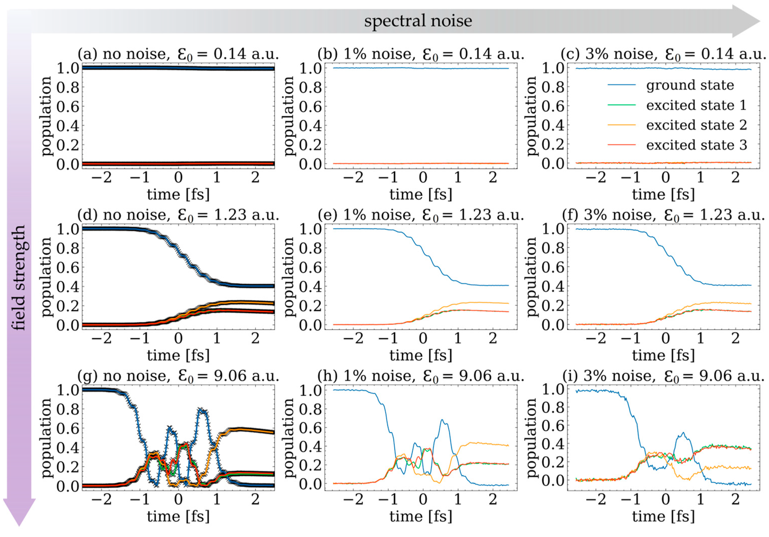
3.2. Line Shape Changes and Population Reconstruction for the Four-Level System

To investigate how more complex electronic population dynamics can be reconstructed with our CNN, we simulate a four-level system, as described in Section 2.1.

The driving pulse, resonant with the central excited state, excites a coherent wavepacket across the three states, where the energy spacing between the excited states is smaller than the spectral bandwidth of the pulse. The resulting absorption spectra for three different field strengths are shown in Figure 7. With an increasing field strength of the pulse, the amplitudes of all three resonances are reduced because of a reduction in the ground state population. As in the two-level system, the resonant excited state stays symmetric, whereas the line shapes of the two other excited states become more asymmetric with increased field strength. As shown in [11], for equal red and blue detuning of the driving pulse, their line shapes become Fano-like with mirrored asymmetries. Small deviations from this asymmetry come from numerical errors due to the discrete spectral grid. The corresponding population dynamics of the four states are shown in Figure 8. The CNN can reconstruct all four state populations for all three field strengths when no noise is added to the OD, compared to the simulated populations (depicted with black markers; see Figure 8a,d,g). Adding noise levels of 1% and 3%, the populations can be reconstructed as well, but only for low and intermediate field strengths; see Figure 8b,c,e,f. For the highest field strength and a 1% noise level, shown in Figure 8h, the reconstructed populations show similar slower dynamics as the simulated populations, but the local minima and maxima of the population transfer are decreased in amplitude when compared to the simulations. When increasing the noise to 3% for the highest field strength, as shown in Figure 8i, many of the predicted population dynamics are not correct with regard to the simulated populations: the fast oscillations are missing, the number of Rabi cycles is reduced and after the pulse is over (t > 1 fs), the populations of the detuned states, e1 (green) and e2 (red), are larger than the resonant excited state population (orange), which is in contrast to the simulated populations. Yet these deviations can only be found for the highest field strengths in the 3% noise case. Overall, the CNN reconstructs the four electronic state populations mostly accurately, as quantified by the mean errors in

Table 2. MSE and MAE of the population reconstruction for the four-level system.

Error	No Noise	1% Noise	3% Noise
MSE	3.6 × 10−8	1.7 × 10−4	1.3 × 10−3
MAE	1.2 × 10−4	4.4 × 10−3	1.4 × 10−2

. The mean errors are obtained by averaging over the populations of all field strengths; thus, the deviations for the highest field strengths contribute only marginally. As in the two-level system, the errors increase by an order(s) of magnitude when the noise level is increased. Comparing the overall performance to the two-level system and the error values in Table 1, the CNN reconstructs the four-level populations slightly better than for the two-level system, which might be due to the higher amount of information provided in the OD spectra.

4. Conclusions and Outlook

In summary, we have shown that a CNN can be used to reconstruct time-dependent electronic state populations from simulated OD spectra for two different scenarios of laser pulse excitations: the excitation of an individual electronic state (in the two-level system) as well as launching an electronic wave packet consisting of three excited states (in the four-level system). We have demonstrated this for driving pulse electric-field strengths spanning across two orders of magnitude—continuously tuning from the weak-field to the strong-coupling case. For the two-level system, we have further shown that reconstruction is possible for (two) different cases of pulse detunings. Furthermore, by including two different noise levels in the input spectra, we have found that a 1% noise level does not change the CNN reconstructions significantly, whereas an increase to a 3% noise level leads to the CNN predictions deviating more significantly from the input populations for the highest driving pulse field strengths. With regards to the pulse intensities and dipole couplings chosen here, we thus identify the 3% noise level as an upper limit. In the future, for utilizing the CNN for experimental strong-field-driven absorption spectra, we suggest a dataset combining theoretical simulations and experimental weak-field absorption measurements—where the populations are nearly unchanged and could be calculated with perturbation theory—which is conceptually similar to previous works [21,23,24,25,27,28,30,33]. In the XUV spectral regime, strong coupling experiments have been performed with self-amplified spontaneous emission (SASE) [4]-based FEL pulses in an autoionizing state [9]. In these cases, not only the peak intensity but also the spectral structure, central photon energy and pulse duration vary from shot to shot. The models and datasets discussed here should thus be expanded to higher dimensions by also training the CNN on this extended parameter space. To that end, the measurements should account for these different input parameters instead of averaging over them to provide large enough datasets. As a possible benefit of this, the CNN might be capable of learning and predicting FEL pulse parameters in parallel with the populations or could be combined with other neural networks (NNs) trained for FEL pulses [20,24] to achieve this. Alternatively, using more stable and coherent seeded FEL pulses [39], the simulation and CNN presented here could already be sufficient to predict the electronic state populations, but such experiments have not been performed yet. Furthermore, combinations with noise reduction NNs [26] might be helpful for even more precise predictions. As an outlook, our simulated two-level dynamics reveal absorption changes that in principle allow for a novel method of light amplification (when the OD becomes negative), even without population inversion (cf. Figure 5). In previous work, light amplification was achieved by population inversion [14], stimulated Raman scattering [40,41], phase shifts through mechanical displacement [42] or by including additional states/ionization continua or light fields in the case of amplification without population inversion [34,43,44,45,46,47,48,49,50,51,52]. In most cases, the electron populations play a key role. Thus, we expect that our approach of a few-level-based simulation and CNN will also help in the future to investigate different light amplification mechanisms. In addition, the population dynamics of the coherent wavepacket excitation in the four-level system illustrate how intra-pulse electronic population transfer leads to absorption changes when more than a single resonance in an atom is involved. Going one step further by exciting or ionizing (several) electronic states in molecules could ultimately lead to ultrafast charge transfer dynamics [15,17,53], where we expect a CNN to provide predictions of electronic populations during the pulse duration—which might influence subsequent charge transfer and even slower molecular structural dynamics—perhaps in combination with corresponding CNNs [27,28,29,30]. Overall, strong-field-modified absorption spectra can be used to investigate electronic dynamics in atoms and molecules, which—in turn—can also be used to shape and modify the driving pulses themselves, such as their amplification in selected spectral regions. In the future, we expect ML in general and CNNs in particular to provide new insights into the ultrafast interplay of UV, XUV and X-ray laser pulses with atoms or molecules.

References

1. Hentschel, M.; Kienberger, R.; Spielmann, C.; Reider, G.A.; Milosevic, N.; Brabec, T.; Corkum, P.; Heinzmann, U.; Drescher, M.; Krausz, F. Attosecond Metrology. Nature 2001, 414, 509–513. [Google Scholar] [CrossRef]
2. Lewenstein, M.; Balcou, P.; Ivanov, M.Y.; L’Huillier, A.; Corkum, P.B. Theory of High-Harmonic Generation by Low-Frequency Laser Fields. Phys. Rev. A 1994, 49, 2117. [Google Scholar] [CrossRef]
3. Paul, P.M.; Toma, E.S.; Breger, P.; Mullot, G.; Augé, F.; Balcou, P.; Muller, H.G.; Agostini, P. Observation of a Train of Attosecond Pulses from High Harmonic Generation. Science 2001, 292, 1689–1692. [Google Scholar] [CrossRef] [PubMed]
4. Ackermann, W.; Asova, G.; Ayvazyan, V.; Azima, A.; Baboi, N.; Bähr, J.; Balandin, V.; Beutner, B.; Brandt, A.; Bolzmann, A.; et al. Operation of a Free-Electron Laser from the Extreme Ultraviolet to the Water Window. Nat. Photonics 2007, 1, 336–342. [Google Scholar] [CrossRef]
5. Duris, J.; Li, S.; Driver, T.; Champenois, E.G.; MacArthur, J.P.; Lutman, A.A.; Zhang, Z.; Rosenberger, P.; Aldrich, J.W.; Coffee, R.; et al. Tunable Isolated Attosecond X-Ray Pulses with Gigawatt Peak Power from a Free-Electron Laser. Nat. Photonics 2019, 14, 30–36. [Google Scholar] [CrossRef]
6. Maroju, P.K.; Grazioli, C.; Di Fraia, M.; Moioli, M.; Ertel, D.; Ahmadi, H.; Plekan, O.; Finetti, P.; Allaria, E.; Giannessi, L.; et al. Attosecond Pulse Shaping Using a Seeded Free-Electron Laser. Nature 2020, 578, 386–391. [Google Scholar] [CrossRef]
7. Tzallas, P.; Skantzakis, E.; Nikolopoulos, L.A.A.; Tsakiris, G.D.; Charalambidis, D. Extreme-Ultraviolet Pump–Probe Studies of One-Femtosecond-Scale Electron Dynamics. Nat. Phys. 2011, 7, 781–784. [Google Scholar] [CrossRef]
8. Nandi, S.; Olofsson, E.; Bertolino, M.; Carlström, S.; Zapata, F.; Busto, D.; Callegari, C.; Di Fraia, M.; Eng-Johnsson, P.; Feifel, R.; et al. Observation of Rabi Dynamics with a Short-Wavelength Free-Electron Laser. Nature 2022, 608, 488–493. [Google Scholar] [CrossRef]
9. Ott, C.; Aufleger, L.; Ding, T.; Rebholz, M.; Magunia, A.; Hartmann, M.; Stooß, V.; Wachs, D.; Birk, P.; Borisova, G.D.; et al. Strong-Field Extreme-Ultraviolet Dressing of Atomic Double Excitation. Phys. Rev. Lett. 2019, 123, 163–201. [Google Scholar] [CrossRef]
10. Aufleger, L.; Friebel, P.; Rupprecht, P.; Magunia, A.; Ding, T.; Rebholz, M.; Hartmann, M.; Ott, C.; Pfeifer, T. Line-Shape Broadening of an Autoionizing State in Helium at High XUV Intensity. New J. Phys. 2022, 24, 013014. [Google Scholar] [CrossRef]
11. Magunia, A.; Aufleger, L.; Ding, T.; Rupprecht, P.; Rebholz, M.; Ott, C.; Pfeifer, T. Bound-State Electron Dynamics Driven by Near-Resonantly Detuned Intense and Ultrashort Pulsed XUV Fields. Appl. Sci. 2020, 10, 6153. [Google Scholar] [CrossRef]
12. He, Y.; Shi, H.; Xue, N.; Magunia, A.; Sun, S.; Ding, J.; Hu, B.; Liu, Z. Direct Manipulation of Atomic Excitation with Intense Extreme-Ultraviolet Laser Fields. Phys. Rev. A 2022, 105, 043113. [Google Scholar] [CrossRef]
13. Stooß, V.; Cavaletto, S.M.; Donsa, S.; Blättermann, A.; Birk, P.; Keitel, C.H.; Březinová, I.; Burgdörfer, J.; Ott, C.; Pfeifer, T. Real-Time Reconstruction of the Strong-Field-Driven Dipole Response. Phys. Rev. Lett. 2018, 121, 173005. [Google Scholar] [CrossRef]
14. Rohringer, N.; Ryan, D.; London, R.A.; Purvis, M.; Albert, F.; Dunn, J.; Bozek, J.D.; Bostedt, C.; Graf, A.; Hill, R.; et al. Atomic Inner-Shell X-Ray Laser at 1.46 Nanometres Pumped by an X-Ray Free-Electron Laser. Nature 2012, 481, 488–491. [Google Scholar] [CrossRef]
15. Calegari, F.; Ayuso, D.; Trabattoni, A.; Belshaw, L.; De Camillis, S.; Anumula, S.; Frassetto, F.; Poletto, L.; Palacios, A.; Decleva, P.; et al. Ultrafast Electron Dynamics in Phenylalanine Initiated by Attosecond Pulses. Science 2014, 346, 336–339. [Google Scholar] [CrossRef]
16. Mayer, D.; Lever, F.; Picconi, D.; Metje, J.; Alisauskas, S.; Calegari, F.; Düsterer, S.; Ehlert, C.; Feifel, R.; Niebuhr, M.; et al. Following Excited-State Chemical Shifts in Molecular Ultrafast x-Ray Photoelectron Spectroscopy. Nat. Commun. 2022, 13, 198. [Google Scholar] [CrossRef]
17. Al-Haddad, A.; Oberli, S.; González-Vázquez, J.; Bucher, M.; Doumy, G.; Ho, P.; Krzywinski, J.; Lane, T.J.; Lutman, A.; Marinelli, A.; et al. Observation of Site-Selective Chemical Bond Changes via Ultrafast Chemical Shifts. Nat. Commun. 2022, 13, 7170. [Google Scholar] [CrossRef]
18. Cheng, B.; Titterington, D.M. Neural Networks: A Review from a Statistical Perspective. Stat. Sci. 1994, 9, 2–30. [Google Scholar] [CrossRef]
19. Salmela, L.; Tsipinakis, N.; Foi, A.; Billet, C.; Dudley, J.M.; Genty, G. Predicting Ultrafast Nonlinear Dynamics in Fibre Optics with a Recurrent Neural Network. Nat. Mach. Intell. 2021, 3, 344–354. [Google Scholar] [CrossRef]
20. Sanchez-Gonzalez, A.; Micaelli, P.; Olivier, C.; Barillot, T.R.; Ilchen, M.; Lutman, A.A.; Marinelli, A.; Maxwell, T.; Achner, A.; Agåker, M.; et al. Accurate Prediction of X-Ray Pulse Properties from a Free-Electron Laser Using Machine Learning. Nat. Commun. 2017, 8, 15461. [Google Scholar] [CrossRef] [PubMed]
21. Kleinert, S.; Morgner, U.; Tajalli, A.; Nagy, T. Rapid Phase Retrieval of Ultrashort Pulses from Dispersion Scan Traces Using Deep Neural Networks. Opt. Lett. 2019, 44, 979–982. [Google Scholar] [CrossRef]
22. DeLong, K.W.; Ladera, C.L.; Fittinghoff, D.N.; Krumbügel, M.A.; Trebino, R.; Sweetser, J.N. Direct Ultrashort-Pulse Intensity and Phase Retrieval by Frequency-Resolved Optical Gating and a Computational Neural Network. Opt. Lett. 1996, 21, 143–145. [Google Scholar] [CrossRef]
23. Zahavy, T.; Dikopoltsev, A.; Cohen, O.; Mannor, S.; Segev, M. Deep Learning Reconstruction of Ultrashort Pulses. Optica 2018, 5, 666–673. [Google Scholar] [CrossRef]
24. Breckwoldt, N.; Son, S.-K.; Mazza, T.; Rörig, A.; Boll, R.; Meyer, M.; LaForge, A.C.; Mishra, D.; Berrah, N.; Santra, R. Machine-Learning Calibration of Intense x-Ray Free-Electron-Laser Pulses Using Bayesian Optimization. Phys. Rev. Res. 2023, 5, 023114. [Google Scholar] [CrossRef]
25. Gherman, A.M.M.; Kovács, K.; Cristea, M.V.; Toşa, V. Artificial Neural Network Trained to Predict High-Harmonic Flux. Appl. Sci. 2018, 8, 2106. [Google Scholar] [CrossRef]
26. Gutberlet, T.; Chang, H.-T.; Zayko, S.; Sivis, M.; Ropers, C. High-Sensitivity Extreme-Ultraviolet Transient Absorption Spectroscopy Enabled by Machine Learning. Opt. Express 2023, 31, 39757–39764. [Google Scholar] [CrossRef]
27. Shvetsov-Shilovski, N.I.; Lein, M. Deep Learning for Retrieval of the Internuclear Distance in a Molecule from Interference Patterns in Photoelectron Momentum Distributions. Phys. Rev. A 2022, 105, L021102. [Google Scholar] [CrossRef]
28. Liu, X.; Amini, K.; Sanchez, A.; Belsa, B.; Steinle, T.; Biegert, J. Machine Learning for Laser-Induced Electron Diffraction Imaging of Molecular Structures. Commun. Chem. 2021, 4, 154. [Google Scholar] [CrossRef]
29. Rupp, M.; Tkatchenko, A.; Müller, K.R.; Von Lilienfeld, O.A. Fast and Accurate Modeling of Molecular Atomization Energies with Machine Learning. Phys. Rev. Lett. 2012, 108, 058301. [Google Scholar] [CrossRef]
30. Shvetsov-Shilovski, N.I.; Lein, M. Transfer Learning, Alternative Approaches, and Visualization of a Convolutional Neural Network for Retrieval of the Internuclear Distance in a Molecule from Photoelectron Momentum Distributions. Phys. Rev. A 2023, 107, 033106. [Google Scholar] [CrossRef]
31. Brockherde, F.; Vogt, L.; Li, L.; Tuckerman, M.E.; Burke, K.; Müller, K.-R. By-Passing the Kohn-Sham Equations with Machine Learning. Nat. Commun. 2016, 8, 872. [Google Scholar] [CrossRef]
32. Snyder, J.C.; Rupp, M.; Hansen, K.; Müller, K.R.; Burke, K. Finding Density Functionals with Machine Learning. Phys. Rev. Lett. 2012, 108, 253002. [Google Scholar] [CrossRef]
33. Mills, K.; Spanner, M.; Tamblyn, I. Deep Learning and the Schrödinger Equation. Phys. Rev. A 2017, 96, 042113. [Google Scholar] [CrossRef]
34. Ott, C.; Kaldun, A.; Raith, P.; Meyer, K.; Laux, M.; Evers, J.; Keitel, C.-H.; Greene, C.-H.; Pfeifer, T. Lorentz Meets Fano in Spectral Line Shapes: A Universal Phase and Its Laser Control. Science 2013, 340, 716–720. [Google Scholar] [CrossRef]
35. Rupprecht, P.; Aufleger, L.; Heinze, S.; Magunia, A.; Ding, T.; Rebholz, M.; Amberg, S.; Mollov, N.; Henrich, F.; Haverkort, M.W.; et al. Resolving Vibrations in a Polyatomic Molecule with Femtometer Precision via X-Ray Spectroscopy. Phys. Rev. A 2023, 108, 032816. [Google Scholar] [CrossRef]
36. Kingma, D.P.; Lei Ba, J. Adam: A method for stochastic optimization. arXiv 2017, arXiv:1412.6980. [Google Scholar]
37. Fano, U. Effects of Configuration Interaction on Intensities and Phase Shifts. Phys. Rev. 1961, 124, 1866–1878. [Google Scholar] [CrossRef]
38. Rabi, I.I. Space Quantization in a Gyrating Magnetic Field. Phys. Rev. 1937, 51, 652–654. [Google Scholar] [CrossRef]
39. Allaria, E.; Appio, R.; Badano, L.; Barletta, W.A.; Bassanese, S.; Biedron, S.G.; Borga, A.; Busetto, E.; Castronovo, D.; Cinquegrana, P.; et al. Highly Coherent and Stable Pulses from the FERMI Seeded Free-Electron Laser in the Extreme Ultraviolet. Nat. Photonics 2012, 6, 699–704. [Google Scholar] [CrossRef]
40. Weninger, C.; Purvis, M.; Ryan, D.; London, R.A.; Bozek, J.D.; Bostedt, C.; Graf, A.; Brown, G.; Rocca, J.J.; Rohringer, N. Stimulated Electronic X-Ray Raman Scattering. Phys. Rev. Lett. 2013, 111, 233902. [Google Scholar] [CrossRef]
41. Li, K.; Labeye, M.; Ho, P.J.; Gaarde, M.B.; Young, L. Resonant Propagation of x Rays from the Linear to the Nonlinear Regime. Phys. Rev. A 2020, 102, 053113. [Google Scholar] [CrossRef]
42. Heeg, K.P.; Kaldun, A.; Strohm, C.; Reiser, P.; Ott, C.; Subramanian, R.; Lentrodt, D.; Haber, J.; Wille, H.C.; Goerttler, S.; et al. Spectral Narrowing of X-Ray Pulses for Precision Spectroscopy with Nuclear Resonances. Science 2017, 357, 375–378. [Google Scholar] [CrossRef]
43. Gao, J.; Guo, C.; Guo, X.; Jin, G.; Wang, P.; Zhao, J.; Zhang, H.; Jiang, Y.; Wang, D.; Jiang, D. Observation of Light Amplification without Population Inversion in Sodium. Opt. Commun. 1992, 93, 323–327. [Google Scholar] [CrossRef]
44. Grynberg, G.; Pinard, M.; Mandel, P. Amplification without Population Inversion in a V Three-Level System: A Physical Interpretation. Phys. Rev. A 1996, 54, 776. [Google Scholar] [CrossRef]
45. Van Der Veer, W.E.; Van Diest, R.J.J.; Dönszelmann, A.; Van Linden Van Den Heuvell, H.B. Experimental Demonstration of Light Amplification without Population Inversion. Phys. Rev. Lett. 1993, 70, 3243. [Google Scholar] [CrossRef]
46. Zibrov, A.S.; Lukin, M.D.; Nikonov, D.E.; Hollberg, L.; Scully, M.O.; Velichansky, V.L.; Robinson, H.G. Experimental Demonstration of Laser Oscillation without Population Inversion via Quantum Interference in Rb. Phys. Rev. Lett. 1995, 75, 1499. [Google Scholar] [CrossRef]
47. Wen, P.Y.; Kockum, A.F.; Ian, H.; Chen, J.C.; Nori, F.; Hoi, I.C. Reflective Amplification without Population Inversion from a Strongly Driven Superconducting Qubit. Phys. Rev. Lett. 2018, 120, 063603. [Google Scholar] [CrossRef]
48. Kocharovskaia, O.A.; Khanin, I.I. Coherent Amplification of an Ultrashort Pulse in a Three-Level Medium without Population Inversion. Pisma V Zhurnal Eksperimentalnoi I Teor. Fiz. 1988, 48, 581–584. [Google Scholar]
49. Kocharovskaya, O. Amplification and Lasing without Inversion. Phys. Rep. 1992, 219, 175–190. [Google Scholar] [CrossRef]
50. Kocharovskaya, O.; Mandel, P. Amplification without Inversion: The Double-Λ Scheme. Phys. Rev. A 1990, 42, 523. [Google Scholar] [CrossRef]
51. Lyras, A.; Tang, X.; Lambropoulos, P.; Zhang, J. Radiation Amplification through Autoionizing Resonances without Population Inversion. Phys. Rev. A 1989, 40, 4131. [Google Scholar] [CrossRef] [PubMed]
52. Arkhipkin, V.G.; Heller, Y.I. Radiation Amplification without Population Inversion at Transitions to Autoionizing States. Phys. Lett. A 1983, 98, 12–14. [Google Scholar] [CrossRef]
53. Sansone, G.; Kelkensberg, F.; Pérez-Torres, J.F.; Morales, F.; Kling, M.F.; Siu, W.; Ghafur, O.; Johnsson, P.; Swoboda, M.; Benedetti, E.; et al. Electron Localization Following Attosecond Molecular Photoionization. Nature 2010, 465, 763–766. [Google Scholar] [CrossRef] [PubMed]
Figure 1. Conceptual overview of the population reconstruction from absorption changes in a two-level system. (a,b) A laser pulse (violet) excites a two-level system from its electronic ground (blue) state to an excited state (green)—either resonantly (a) or with a small detuning (b). (c) Time-dependent populations of the ground (blue) and excited state (green) for the resonant excitation are simulated with the numerical model. (d) Same as (c) but for the detuned case. (e) The excitation of the two-level system leads to a dipole response (blue) interfering with the incoming laser pulse (violet). (fh) A spectroscopic measurement of these signals leads to a resonance line in the optical density for a weak (ε0 = 0.7 a.u.) and resonant pulse (f), a strongly coupling (ε0 = 6.1 a.u.) and resonant pulse (g) or a strongly coupling (ε0 = 6.1 a.u.) and detuned pulse (h). The natural line shape (f) is modified due to the strong driving fields (g,h), which we use to train the CNN (i) to predict the state populations of the two states (c,d).
Optics 05 00007 g001
Figure 2. Overview of the convolutional neural network structure (for the two-level system). On the left, the sequence of layers is shown. On the right, the (output) array sizes for each layer are given.
Optics 05 00007 g002
Figure 3. Loss (MSE) as a function of training dataset size for (a) the two-level system and (b) the four-level system. In both panels, the models trained on data without noise are shown in blue, the 1% noise cases are shown in green and the 3% noise cases are shown in orange.
Optics 05 00007 g003
Figure 4. Field-strength-dependent OD(ω, ε0) for (a) resonant and (b) detuned driving pulses of the two-level system. The field strength axis is logarithmic to cover the two orders of magnitude of field strength changes. For the resonant case (a), the line shape stays symmetric. In contrast, the line shape becomes asymmetric for the detuned case (b), as discussed in more detail in the text.
Optics 05 00007 g004
Figure 5. Population reconstructions for different noise levels. The same absorption lineout for a detuned driving pulse with a peak field strength of ε0 = 6.1 a.u. is shown for different noise levels: (a) no noise, (b) 1% noise and (c) 3% noise. Simulated populations (black line) are compared to the CNN reconstructions (blue for no noise, green for 1% noise and orange for 3% noise) of the excited (d) and ground states (e).
Optics 05 00007 g005
Figure 6. Field-strength-dependent simulated populations of the excited state for (a) resonant and (b) detuned driving pulses and respective CNN reconstructions (c,d) for the 1% noise level on the ODs. In all panels, the populations are close to zero for low field strengths (ε0 ≤ 1). For higher field strengths (1 a.u. < ε0), the population is first significantly increased and further begins to oscillate up and down when 7 a.u. < ε0. As is well known from Rabi oscillations [38], the population transfer is significantly reduced for detuned pulses; thus, the maximum excited state population for the detuned case (b,d) of Pemax ≈ 0.5 is smaller than for the resonant case (a,c), where Pemax = 1. We do not use the rotating wave approximation; thus, the populations oscillate with 2ωr [38] during the interaction with the pulse, which is twice the frequency of the resonance transition.
Optics 05 00007 g006
Figure 7. Absorption of the four-level system for different field strengths. The OD is shown for a weak field strength, ε0 = 0.1 a.u. (grey), an intermediate field strength, ε0 = 1.2 a.u. (green) and a high field-strength, ε0 = 9.1 a.u. (blue), of the driving pulse. For the high field strength, the OD is multiplied by a factor of 4 for better visibility.
Optics 05 00007 g007
Figure 8. CNN-reconstructed populations of the ground (blue), first excited (green), second excited (orange) and third excited states (red) in the four-level system for (ac) low (ε0 = 0.14 a.u.), (df) intermediate (ε0 = 1.23 a.u.) and (gi) high field strengths (ε0 = 9.06 a.u.) of the pulse, as well as for (a,d,g) no noise, (b,e,h) 1% and (c,f,i) 3% noise. In (a,d,g), the simulated populations are shown with black markers. Similar to the two-level case, the populations stay nearly unchanged for low field strengths but are significantly transferred for higher field strengths and undergo several Rabi oscillations (and faster 2ωr oscillations) for the highest field strength. In all panels, the populations of the two detuned excited states, e1 (green) and e2 (red), are nearly the same, whereas the population of the resonant excited state, e2 (orange), shows clearly different temporal behavior.
Optics 05 00007 g008