
Electromagnetic Multi–Gaussian Speckle


Abstract
:1. Introduction
2. Theory
2.1. Bivariate Complex MG PDF
2.2. The MG Polarization Matrix and Speckle Contrast
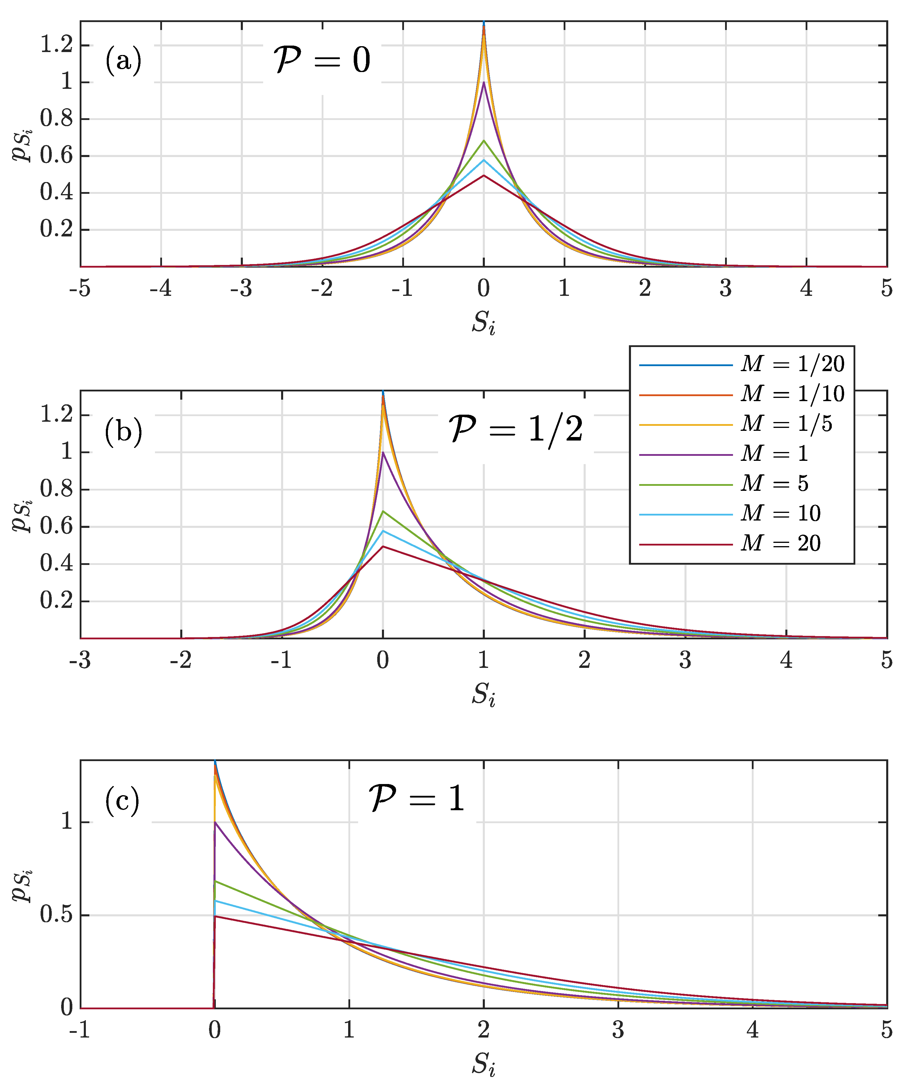
2.3. Instantaneous Stokes Parameter PDFs for MG Speckle
2.3.1.
2.3.2.
2.3.3. and
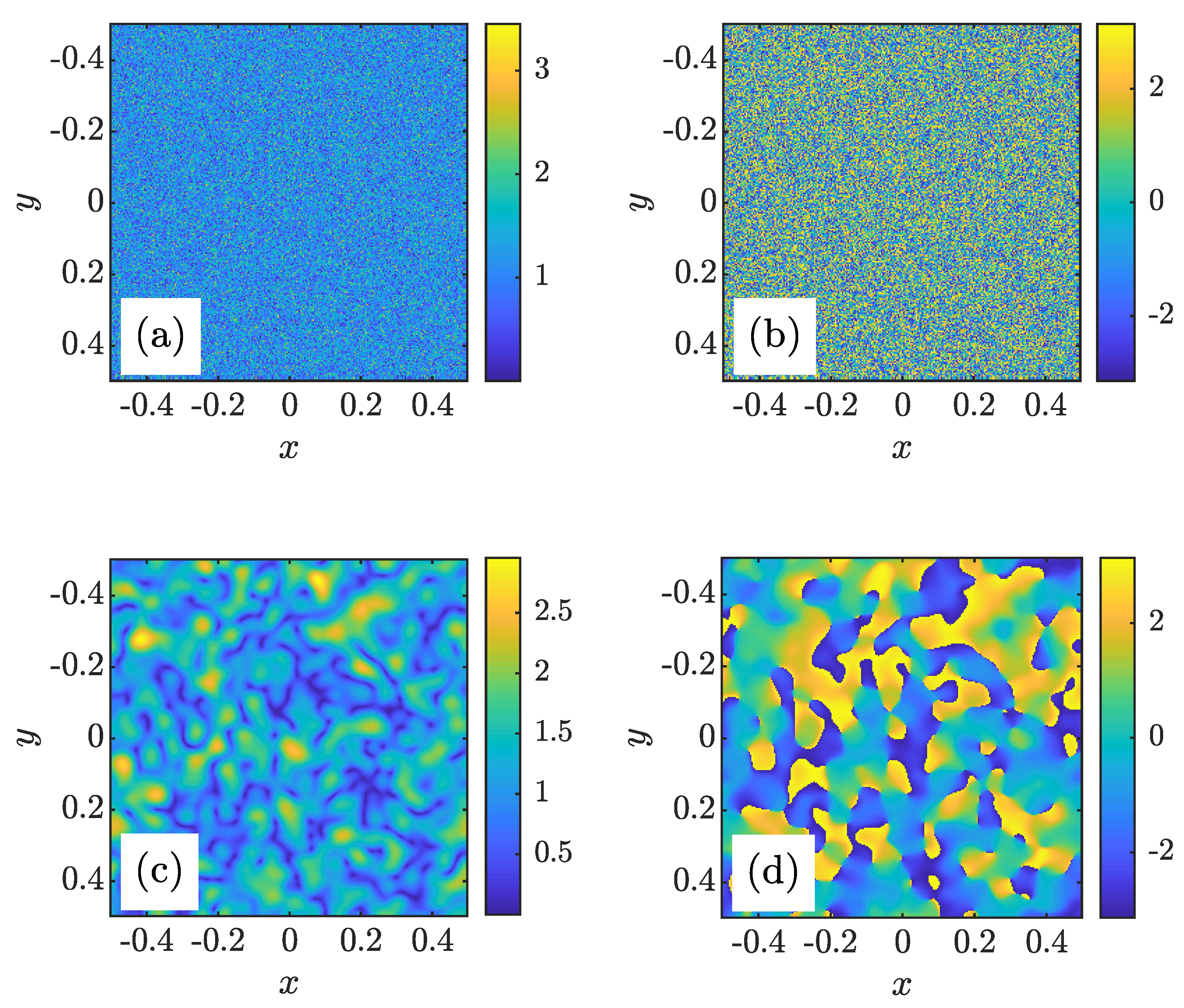
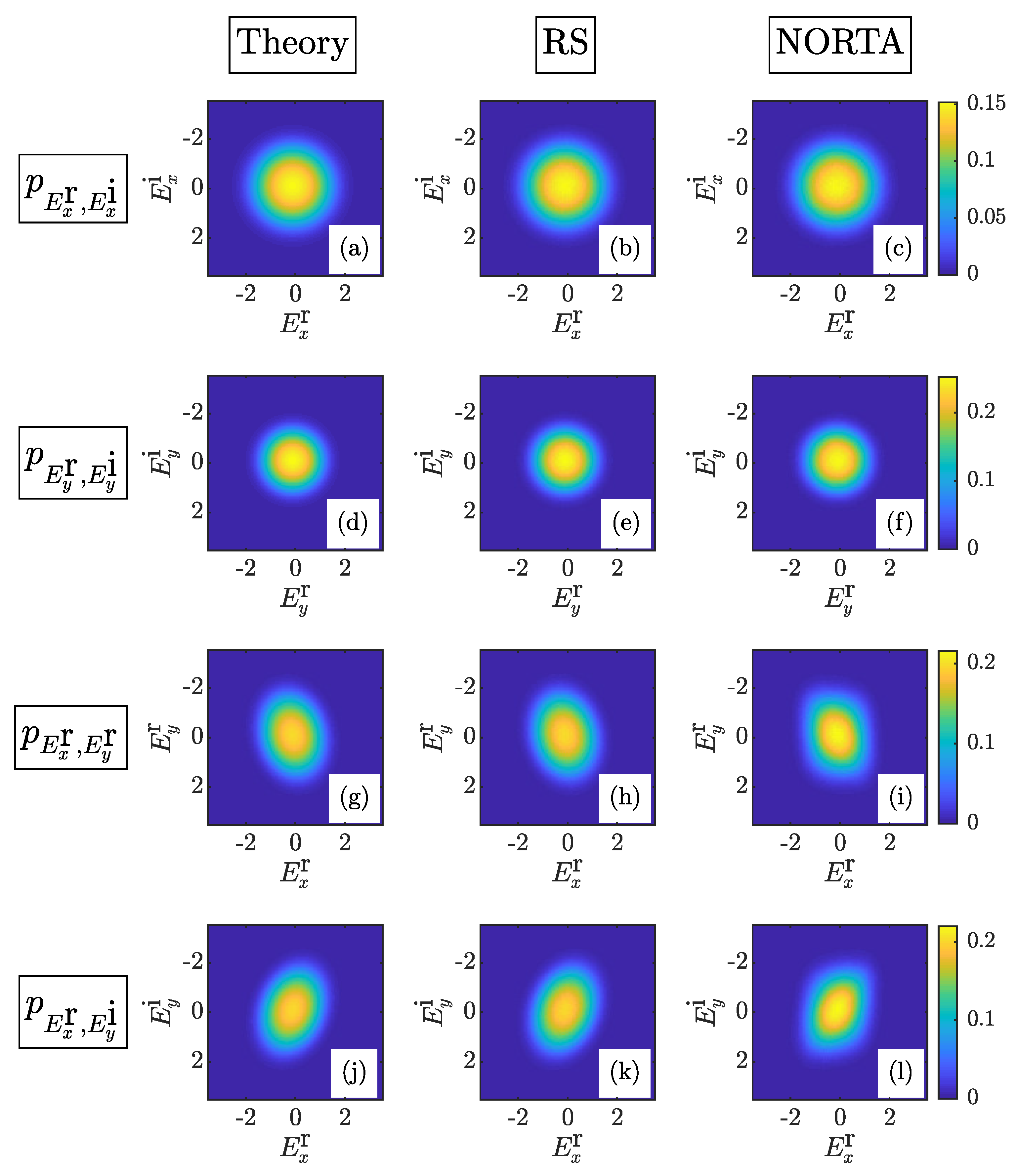
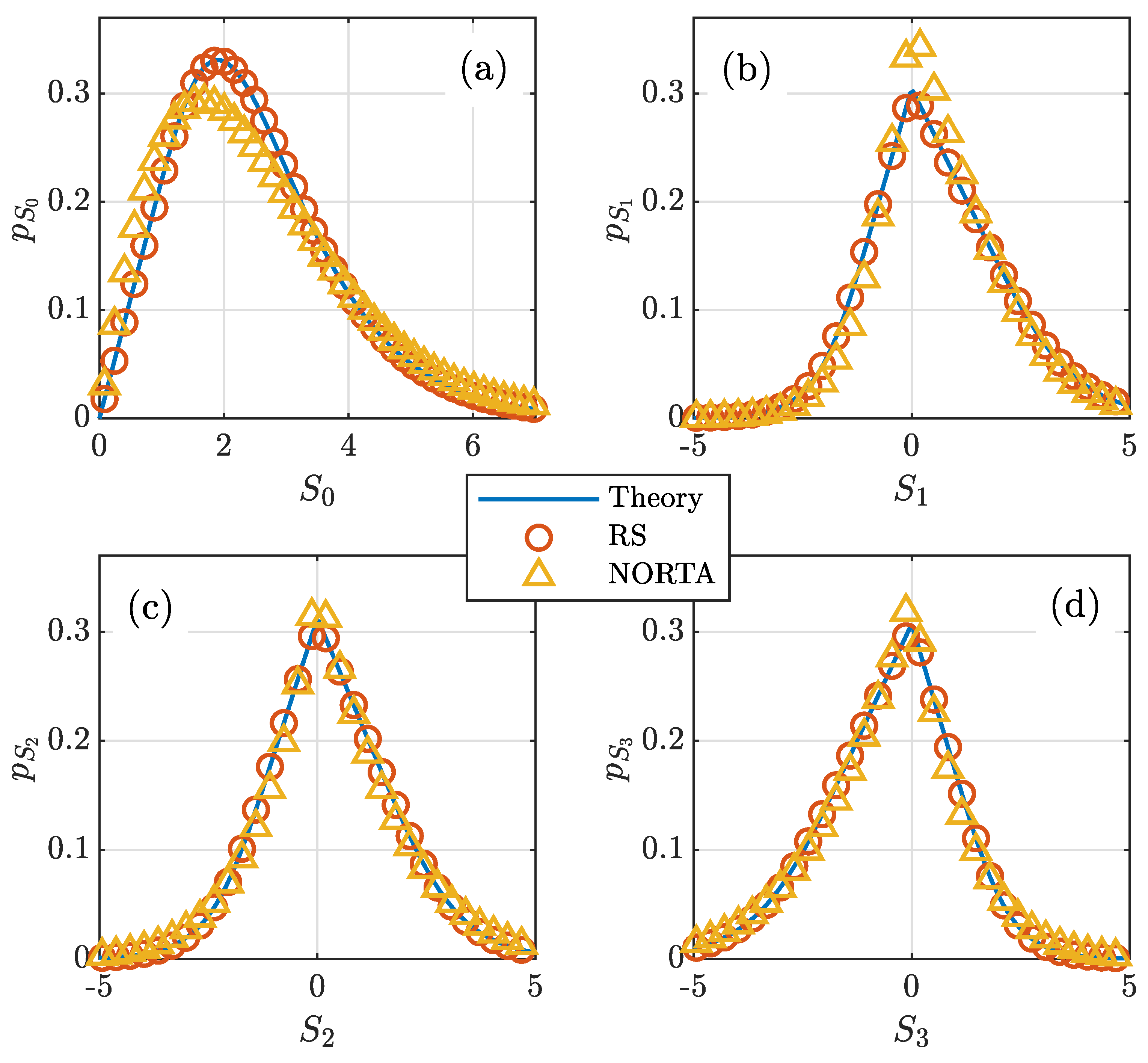
3. Simulation
4. Conclusions
Author Contributions
Funding
Institutional Review Board Statement
Informed Consent Statement
Data Availability Statement
Conflicts of Interest
Abbreviations
| MG | multi-Gaussian |
| probability density function | |
| CCG | circular complex Gaussian |
| RS | rejection sampling |
| NORTA | normal to anything |
References
- Goodman, J. Some effects of target-induced scintillation on optical radar performance. Proc. IEEE 1965, 53, 1688–1700. [Google Scholar] [CrossRef]
- Dainty, J. Some statistical properties of random speckle patterns in coherent and partially coherent illumination. Opt. Acta 1970, 17, 761–772. [Google Scholar] [CrossRef]
- Goodman, J. Statistical properties of laser speckle patterns. In Laser Speckle and Related Phenomena; Topics in Applied Physics; Dainty, J.C., Ed.; Springer: Berlin/Heidelberg, Germany, 1975; Volume 9, pp. 9–75. [Google Scholar]
- Dainty, J. The statistics of speckle patterns. In Progress in Optics; Wolf, E., Ed.; Elsevier: Amsterdam, The Netherlands, 1977; Volume 14, Chapter 1; pp. 1–46. [Google Scholar] [CrossRef]
- Barakat, R. Statistics of the Stokes parameters. J. Opt. Soc. Am. A 1987, 4, 1256–1263. [Google Scholar] [CrossRef]
- Brosseau, C.; Barakat, R.; Rockower, E. Statistics of the Stokes parameters for Gaussian distributed fields. Opt. Commun. 1991, 82, 204–208. [Google Scholar] [CrossRef]
- Eliyahu, D. Vector statistics of correlated Gaussian fields. Phys. Rev. E 1993, 47, 2881–2892. [Google Scholar] [CrossRef] [PubMed]
- Eliyahu, D. Statistics of Stokes variables for correlated Gaussian fields. Phys. Rev. E 1994, 50, 2381–2384. [Google Scholar] [CrossRef]
- Brosseau, C. Fundamentals of Polarized Light: A Statistical Optics Approach; Wiley: New York, NY, USA, 1998. [Google Scholar]
- Santalla del Rio, V.; Pidre Mosquera, J.M.; Isasa, M.V.; de Lorenzo, M.E. Statistics of the degree of polarization. IEEE Trans. Antennas Propag. 2006, 54, 2173–2175. [Google Scholar] [CrossRef]
- Barakat, R. The statistical properties of partially polarized light. Opt. Acta 1985, 32, 295–312. [Google Scholar] [CrossRef]
- Korotkova, O. Changes in statistics of the instantaneous Stokes parameters of a quasi-monochromatic electromagnetic beam on propagation. Opt. Commun. 2006, 261, 218–224. [Google Scholar] [CrossRef]
- Chen, X.; Korotkova, O. Probability density functions of instantaneous Stokes parameters on weak scattering. Opt. Commun. 2017, 400, 1–8. [Google Scholar] [CrossRef]
- Freund, I. ‘1001’ correlations in random wave fields. Waves Random Media 1998, 8, 119–158. [Google Scholar] [CrossRef]
- Dennis, M.R.; O’Holleran, K.; Padgett, M.J. Singular optics: Optical vortices and polarization singularities. In Progress in Optics; Wolf, E., Ed.; Elsevier: Amsterdam, The Netherlands, 2009; Volume 53, Chapter 5; pp. 293–363. [Google Scholar] [CrossRef]
- Shinozuka, M.; Deodatis, G. Simulation of multi-dimensional Gaussian stochastic fields by spectral representation. Appl. Mech. Rev. 1996, 49, 29–53. [Google Scholar] [CrossRef]
- Gbur, G.J. Singular Optics; CRC Press: Boca Raton, FL, USA, 2016. [Google Scholar]
- Goodman, J.W. Speckle Phenomena in Optics: Theory and Applications, 2nd ed.; SPIE Press: Bellingham, WA, USA, 2020. [Google Scholar]
- Raburn, W.S.; Gbur, G. Singularities of partially polarized vortex beams. Front. Phys. 2020, 8, 168. [Google Scholar] [CrossRef]
- Korotkova, O.; Gbur, G. Applications of optical coherence theory. In Progress in Optics; Visser, T.D., Ed.; Elsevier: Amsterdam, The Netherlands, 2020; Volume 65, Chapter 4; pp. 43–104. [Google Scholar] [CrossRef]
- Bender, N.; Yilmaz, H.; Bromberg, Y.; Cao, H. Customizing speckle intensity statistics. Optica 2018, 5, 595–600. [Google Scholar] [CrossRef] [Green Version]
- Bender, N.; Sun, M.; Yilmaz, H.; Bewersdorf, J.; Cao, H. Circumventing the optical diffraction limit with customized speckles. Optica 2021, 8, 122–129. [Google Scholar] [CrossRef]
- Bender, N.; Yilmaz, H.; Bromberg, Y.; Cao, H. Creating and controlling complex light. APL Photonics 2019, 4, 110806. [Google Scholar] [CrossRef]
- Korotkova, O.; Hyde, M.W. Multi-Gaussian random variables for modeling optical phenomena. Opt. Express 2021, 29, 25771–25799. [Google Scholar] [CrossRef] [PubMed]
- Wooding, R.A. The multivariate distribution of complex normal variables. Biometrika 1956, 43, 212–215. [Google Scholar] [CrossRef]
- Goodman, N.R. Statistical analysis based on a certain multivariate complex Gaussian distribution (an introduction). Ann. Math. Stat. 1963, 34, 152–177. [Google Scholar] [CrossRef]
- Wiener, N. Coherency matrices and quantum. J. Math. Phys. 1928, 7, 109–125. [Google Scholar] [CrossRef]
- Wolf, E. Coherence properties of partially polarized electromagnetic radiation. Il Nuovo Cimento 1959, 13, 1165–1181. [Google Scholar] [CrossRef]
- Born, M.; Wolf, E. Principles of Optics: Electromagnetic Theory of Propagation, Interference and Diffraction of Light, 7th ed.; Cambridge University Press: New York, NY, USA, 1999. [Google Scholar]
- Mandel, L.; Wolf, E. Optical Coherence and Quantum Optics; Cambridge University Press: New York, NY, USA, 1995. [Google Scholar]
- Goodman, J.W. Statistical Optics, 2nd ed.; Wiley: Hoboken, NJ, USA, 2015. [Google Scholar]
- Richards, B.; Wolf, E.; Gabor, D. Electromagnetic diffraction in optical systems, II. Structure of the image field in an aplanatic system. Proc. R. Soc. Lond. A 1959, 253, 358–379. [Google Scholar] [CrossRef]
- Novotny, L.; Hecht, B. Principles of Nano-Optics; Cambridge University Press: Cambridge, UK, 2006. [Google Scholar] [CrossRef]
- Goldstein, D. Polarized Light, 3rd ed.; CRC Press: Boca Raton, FL, USA, 2011. [Google Scholar]
- Korotkova, O. Random Light Beams: Theory and Applications; CRC Press: Boca Raton, FL, USA, 2014. [Google Scholar]
- Picinbono, B. Second-order complex random vectors and normal distributions. IEEE Trans. Signal Process. 1996, 44, 2637–2640. [Google Scholar] [CrossRef]
- Kalos, M.H.; Whitlock, P.A. Monte Carlo Methods, 2nd ed.; Wiley-VCH: Weinheim, Germany, 2008. [Google Scholar]
- Grigoriu, M. Crossing of non-Gaussian translation processes. J. Eng. Mech. 1984, 110, 610–620. [Google Scholar] [CrossRef]
- Yamazaki, F.; Shinozuka, M. Digital generation of non-Gaussian stochastic fields. J. Eng. Mech. 1988, 114, 1183–1197. [Google Scholar] [CrossRef]
- Cario, M.C.; Nelson, B.L. Modeling and Generating Random Vectors with Arbitrary Marginal Distributions and Correlation Matrix; Tech. Rep.; Northwestern University: Evanston, IL, USA, 1997. [Google Scholar]
- Yura, H.T.; Hanson, S.G. Digital simulation of an arbitrary stationary stochastic process by spectral representation. J. Opt. Soc. Am. A 2011, 28, 675–685. [Google Scholar] [CrossRef] [PubMed] [Green Version]
- Yura, H.T.; Hanson, S.G. Digital simulation of two-dimensional random fields with arbitrary power spectra and non-Gaussian probability distribution functions. Appl. Opt. 2012, 51, C77–C83. [Google Scholar] [CrossRef] [Green Version]


Publisher’s Note: MDPI stays neutral with regard to jurisdictional claims in published maps and institutional affiliations. |
© 2022 by the authors. Licensee MDPI, Basel, Switzerland. This article is an open access article distributed under the terms and conditions of the Creative Commons Attribution (CC BY) license (https://creativecommons.org/licenses/by/4.0/).
Share and Cite
Hyde, M.W., IV; Korotkova, O. Electromagnetic Multi–Gaussian Speckle. Optics 2022, 3, 19-34. https://doi.org/10.3390/opt3010003
Hyde MW IV, Korotkova O. Electromagnetic Multi–Gaussian Speckle. Optics. 2022; 3(1):19-34. https://doi.org/10.3390/opt3010003
Chicago/Turabian StyleHyde, Milo W., IV, and Olga Korotkova. 2022. "Electromagnetic Multi–Gaussian Speckle" Optics 3, no. 1: 19-34. https://doi.org/10.3390/opt3010003
APA StyleHyde, M. W., IV, & Korotkova, O. (2022). Electromagnetic Multi–Gaussian Speckle. Optics, 3(1), 19-34. https://doi.org/10.3390/opt3010003