Article

Study of Superoscillating Functions Application to Overcome the Diffraction Limit with Suppressed Sidelobes

by
Svetlana N. Khonina
1,2,*,
Ekaterina D. Ponomareva
2 and
Muhammad A. Butt
2,3
1
Image Processing Systems Institute-Branch of the Federal Scientific Research Centre “Crystallography and Photonics” of Russian Academy of Sciences, 443001 Samara, Russia
2
Samara National Research University, 443086 Samara, Russia
3
Institute of Microelectronics and Optoelectronics, Warsaw University of Technology, Koszykowa 75, 00-662 Warszawa, Poland
*
Author to whom correspondence should be addressed.
Optics 2021, 2(3), 155-168; https://doi.org/10.3390/opt2030015
Submission received: 18 June 2021 / Revised: 17 August 2021 / Accepted: 18 August 2021 / Published: 20 August 2021
(This article belongs to the Special Issue Feature Papers in Optics)

Abstract

:
The problem of overcoming the diffraction limit does not have an unambiguously advantageous solution because of the competing nature of different beams’ parameters, such as the focal spot size, energy efficiency, and sidelobe level. The possibility to overcome the diffraction limit with suppressed sidelobes out of the near-field zone using superoscillating functions was investigated in detail. Superoscillation is a phenomenon in which a superposition of harmonic functions contains higher spatial frequencies than any of the terms in the superposition. Two types of superoscillating one-dimensional signals were considered, and simulation of their propagation in the near diffraction zone based on plane waves expansion was performed. A comparative numerical study showed the possibility of overcoming the diffraction limit with a reduced level of sidelobes at a certain distance outside the zone of evanescent waves.

1. Introduction

The problem of the diffraction limit is that the minimum size of a distinguishable object or its part is equal to half of the wavelength of the illuminating radiation, which is a fundamental limitation associated with the diffraction of radiation. Overcoming the diffraction limit determined following Abbe’s theory and the Rayleigh criterion [1] is the topic of several fundamental and applied research in modern optics. The high interest in solving this problem is determined by the many potential applications in improving the quality of optical images, compression of recording on optical storage media, lithography and nanostructuring, optical manipulation up to atomic dimensions, and many other fields.
One of the directions effectively used to achieve super-resolution is near-field optics [2,3,4,5,6,7,8,9,10,11,12]. Near-field optics study fields near a radiation source or an impact surface, which implies consideration of evanescent waves [13,14]. In this case, there are no restrictions on the size of the light spot—the localization of the laser spot can be arbitrarily small [15,16,17,18,19], but this method is not suitable for optical systems intended to transmit information over significant distances.
Another direction, aimed to overcome the diffraction limit outside of the near-field zone, is associated with the concept of a superoscillating field [20,21,22,23,24,25]. In 1952, Toraldo di Francia proposed the concept of super-amplified antennas that can be applied to optical instruments to increase their resolution beyond the diffraction limit [20]. In 1985, Bucklew and Saleh showed that an ideal wide-range imaging system could be used to image 1D binary images with arbitrary resolution at the expense of energy, exhibiting many of the same characteristics as super vibrations [21]. A systematic study of optical superoscillations was recently revived in the context of quantum mechanics after Aharonov et al. showed that weak quantum mechanical measurements could have values outside the spectrum of the corresponding operator [22]. In 2006, Berry and Popescu showed that these superoscillating optical waves could form arbitrarily small spatial energy localizations that propagate far from the source, i.e., without the participation of evanescent waves [23].
However, only a small fraction of the energy of the electromagnetic field can exist in the form of superoscillations. The studies of Ferreira and Kempf showed that the energy that can be directed into the superoscillatory region decreases exponentially with the number of superoscillations [24]. The energy directed into the superoscillatory region also increases with the oscillation speed, but only polynomially. Thus, the price to be paid for overcoming the diffraction limit is a significant increase inside lobes and energy loss [25].
A similar situation occurs with sharp focusing of laser radiation [26,27,28] which leads to limitations in the use of superoscillating filters [29]. Note, however, that by varying the parameters of the incident beam and the focusing system, a compromise solution can be obtained that provides a defined balance between a decrease in the size of the light spot and an increase in sidelobes [30,31].
In this work, the influence of the parameters of the input distribution on the possibility of overcoming the diffraction limit outside the zone of damped waves is studied in detail. Superoscillating signals of two types are discussed: one is based on the superposition of spatial harmonics, and another is composed by the power of the complex function. Numerical modeling is performed using the propagation operator based on the expansion in terms of plane waves.
As a result, it was shown that by varying the parameters, it is possible to overcome the diffraction limit with a reduced level of sidelobes, but only at a certain distance. To control this characteristic as well, additional algorithms are required. In this case, it is important to know the influence of each parameter, which makes the performed studies especially useful.

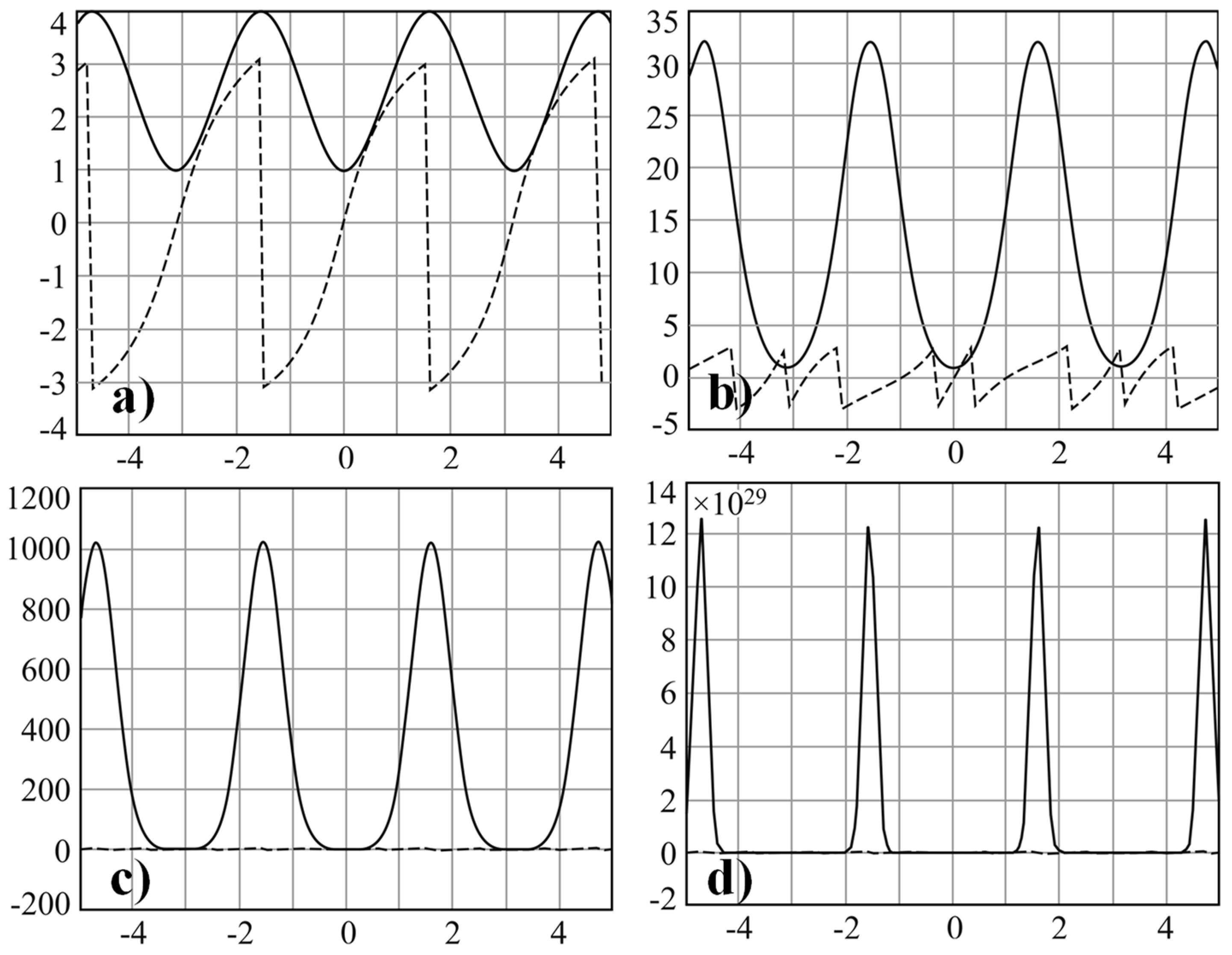
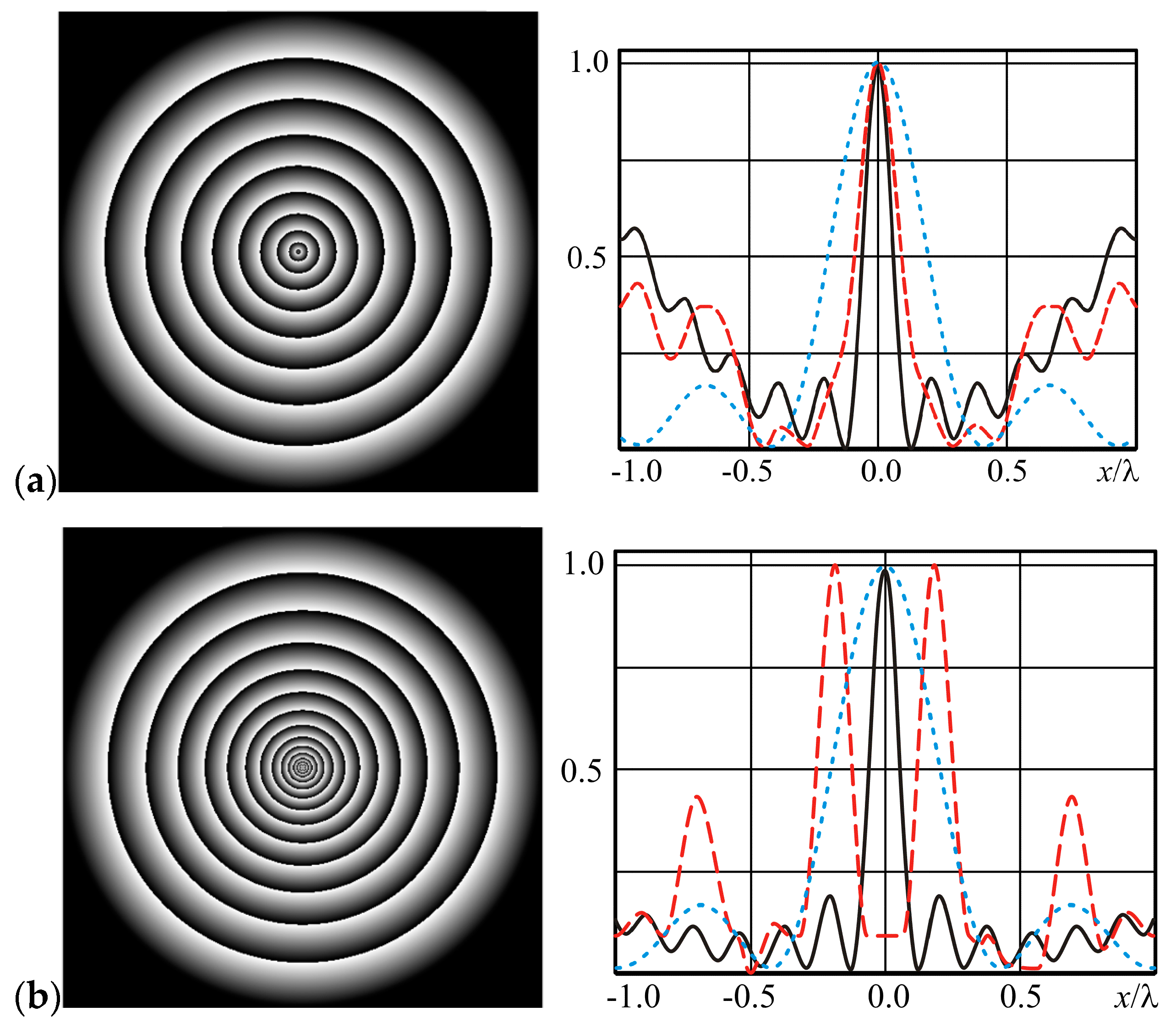
2. Superoscillating Signal Based on Superposition of Spatial Harmonics

An illustrative example of a superoscillating function is the superposition of spatial harmonic functions considered in [32]:
f ( x ) = a n cos ( 2 π n x )
By choosing the correct sequence constants a n , one can create distributions that fluctuate much faster than the highest frequency component. Consider, for example, signal (1) with coefficients: α 0 = 1 , α 1 = 113295000 , α 2 = 30802818 , α 3 = 26581909 , α 4 = 10836909 , α 5 = 1762818 , and α n = 0 at n > 5 . Figure 1 shows a graph of such distribution, x [ 5 λ , 5 λ ] where λ is the radiation wavelength.
To see the features of the field of Equation (1), it is necessary to zoom the region near x = 0 (see Figure 2, bold line). The function (Figure 2, dashed line) is also illustrated for comparison:
f max ( x ) = cos ( 2 π 5 x ) ,
which is the highest-frequency component of the field of Equation (1).
One can notice that the function f(x) oscillates much faster than f max ( x ) from Equation (2). Indeed, near x = 0, the function f(x) from Equation (1) can be well approximated by the harmonic function
f + ( x ) = 0.5 [ cos ( 2 π 43.6 x ) + 1 ] ,
where the coefficient 43.6 is selected so that the difference between f + ( x ) and f(x) is equal to zero on the interval x [ 0.01 ,   0.01 ] . Note that f + ( x ) is oscillating almost 9 times faster than the maximum harmonic of Equation (2). The function of Equation (3) is shown by a thin line in Figure 2.
As seen from Figure 2, the width of the central peak between zero values is less than 0.03λ and slightly more than 0.01λ by full-width at half maximum intensity (FWHM). The size of the central spot is much less than the diffraction limit, which is 0.5λ for free space. If the signal of Equation (1), when propagating over more than the wavelength λ, will allow obtaining a distribution with the central peak size less than the diffraction limit, then the diffraction limit can be overcome using a superoscillating signal of this type.
The simulation of the propagation of the input distributions in free space was carried out based on the plane waves expansion [33]. In the 1D case, the propagation operator has the following form [34]:
F ( u , z ) = T T f ( x ) { α 0 α 0 exp ( i k z 1 α 2 ) exp [ i k α ( u x ) ] d α } d x ,
where f ( x ) is the input signal, limited in the spatial domain by the interval [ T , T ] and in the spectral domain by the interval of spatial frequencies [ α 0 ; α 0 ] , λ is the radiation wavelength, chosen for convenience equal to 1 μm; z is the propagation distance, k = 2π/λ is the wavenumber, F ( u , z ) is the output signal.
The kernel of the propagation operator of Equation (4) contains the weight function:
exp ( i k z 1 α 2 ) = { exp ( k z α 2 1 ) , | α | > 1 ; exp ( i k z 1 α 2 ) , | α | < 1 .
It can be seen from Equation (5) that field components of Equation (1), the spatial frequencies of which | α | > 1 , are exponentially suppressed exp ( 2 π z λ α 2 1 ) at z > 0.3λ. Thus, the survival region of evanescent waves is limited by the propagation distance z < 0.3λ.
Let us first consider the possibility of overcoming the diffraction limit using the superoscillating function of Equation (1) at a distance z = 0.5λ.
The spatial spectrum of the field of Equation (1), which is described by the expression P ( α ) = T T f ( x ) exp ( i k α x ) d x , is shown in Figure 3: Figure 3a corresponds to the original spectrum ( α 0 = 6), and Figure 3b to the spectrum truncated by a function of Equation (5) at z = 0.5λ.
The field calculated after propagation to the distance z = 0.5λ using the operator of Equation (4) is shown in Figure 4. The horizontal line in Figure 4 shows the interval size equal to 0.5λ (diffraction limit) for comparison with the FWHM size. As can be seen from Figure 4, the size of the central peak is less than the diffraction limit. Next, the propagation of the field of Equation (1) is much further than the region of evanescent waves is discussed. In this case, it makes no sense to consider spatial frequencies significantly exceeding 1 since the spectrum is automatically truncated by the function of Equation (5); therefore, in further research, α 0 = 1.5 is used.
The results of calculating the field of Equation (4) propagation over a distance up to z = 100λ are shown in Figure 5. As can be seen, although the field changes somewhat, the central peak retains its size below the diffraction limit. Note that to obtain such a result, it is necessary to consider the input field of Equation (1) over a significant spatial interval (in this case, T = 25λ was used). At small sizes of the input field, overcoming the diffraction limit at distances z > 5λ is not observed.
Thus, a superoscillating field of Equation (1) can be used to overcome the diffraction limit outside the region of evanescent waves, considering the significant size of the input field. Note, however, that in the obtained distributions, the central peak is too closely surrounded by sidelobes of approximately the same height. The use of such distributions is inconvenient even in scanning optical systems. Therefore, another type of superoscillating field is considered.

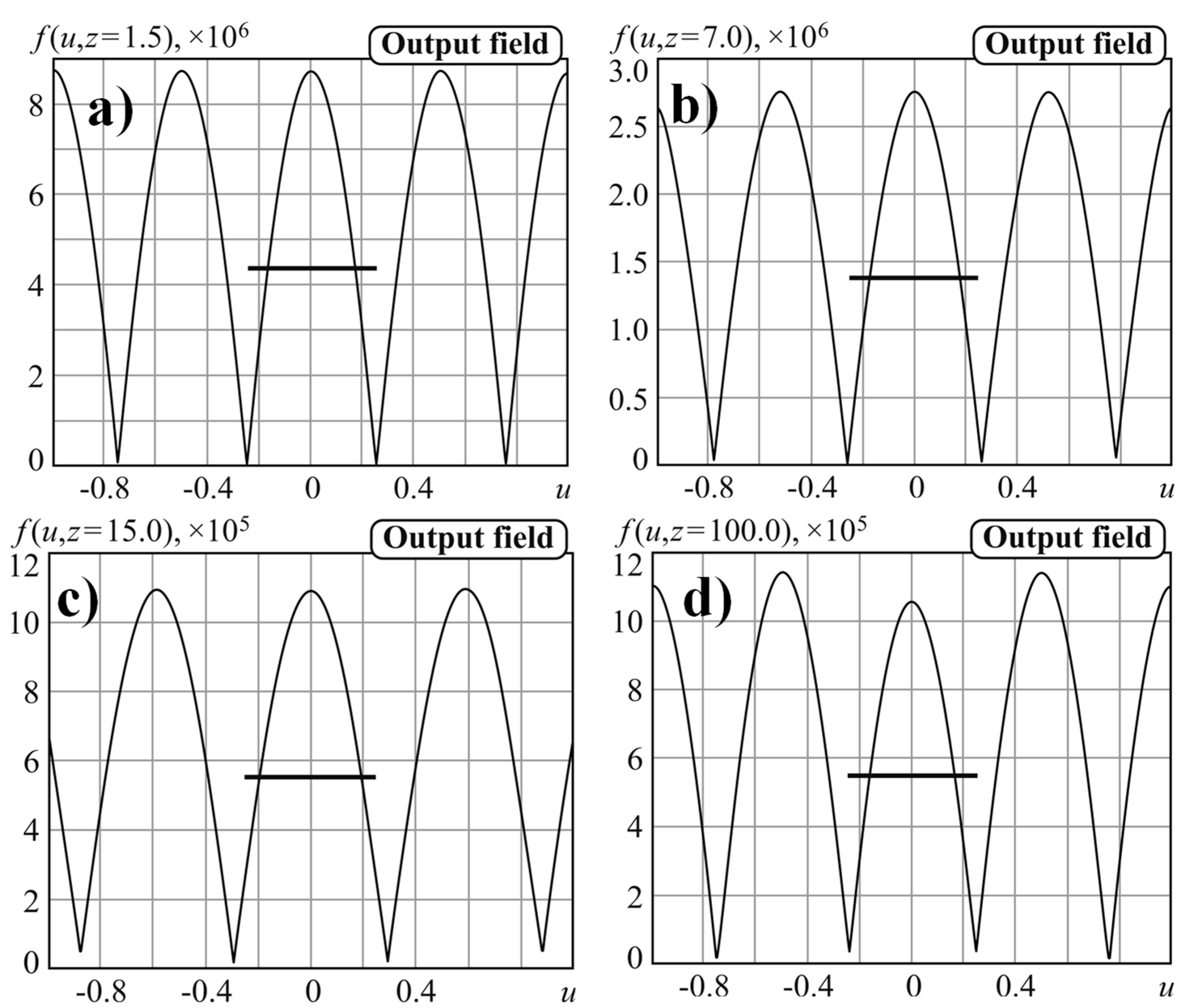
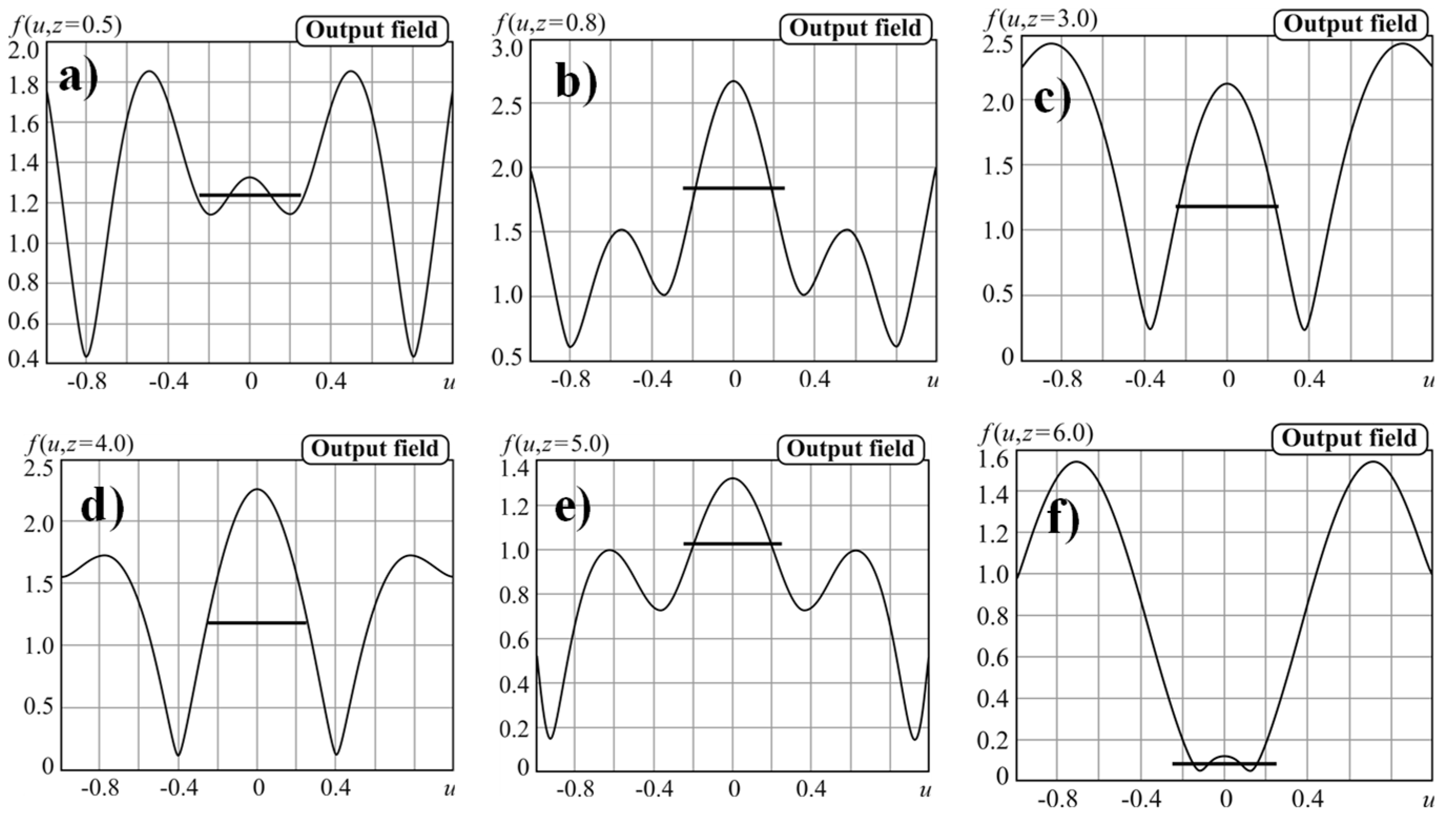
3. Superoscillating Field Based on the Power of the Complex Function
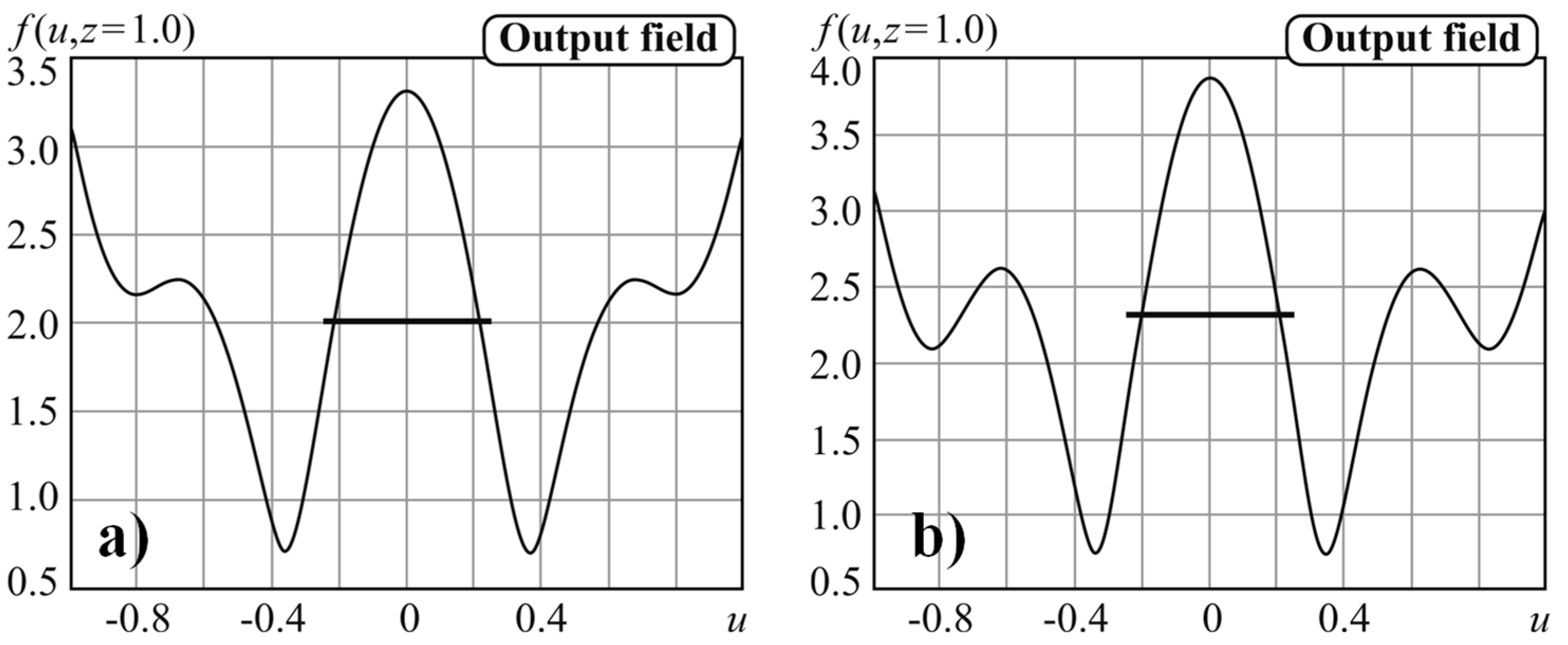
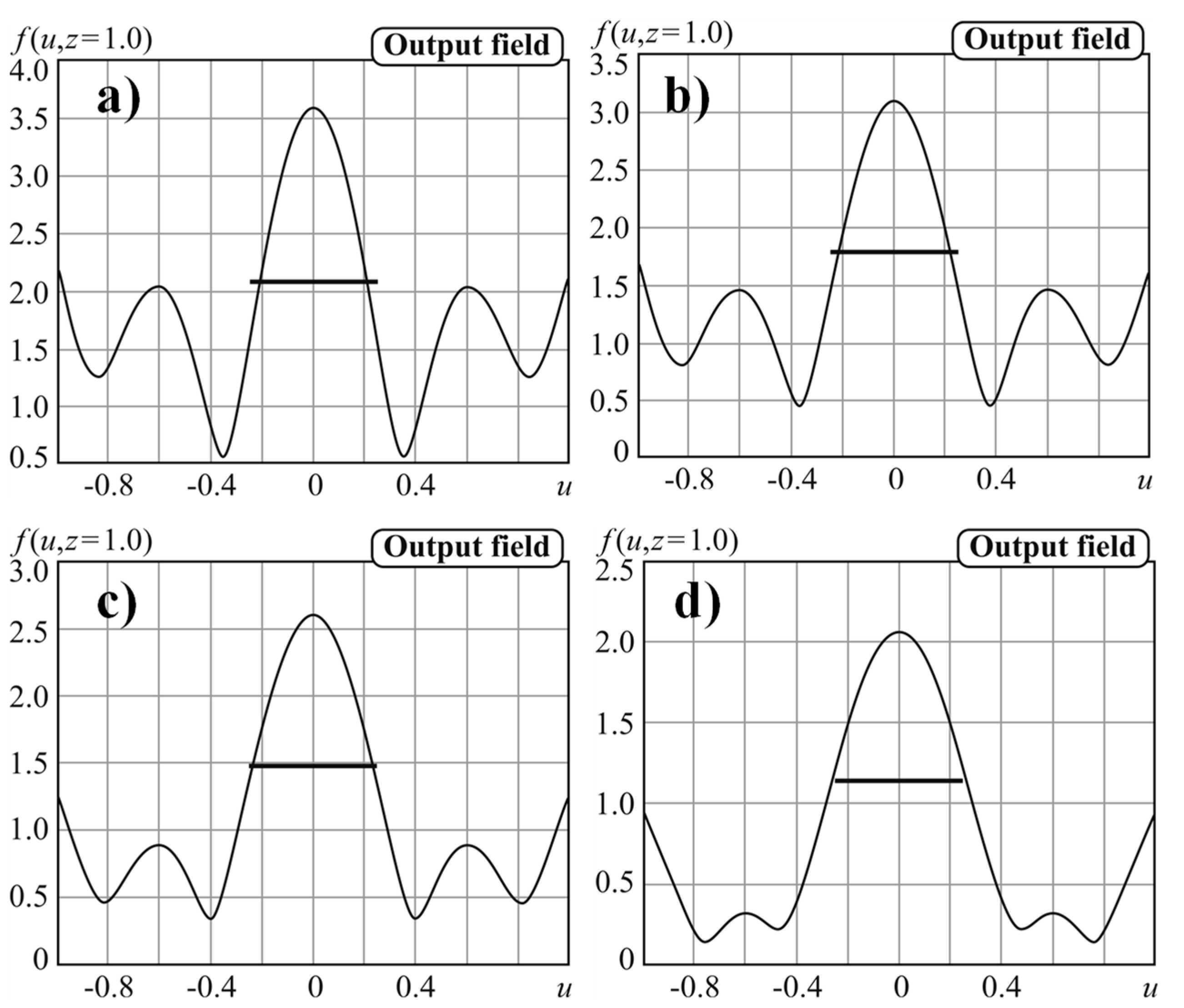
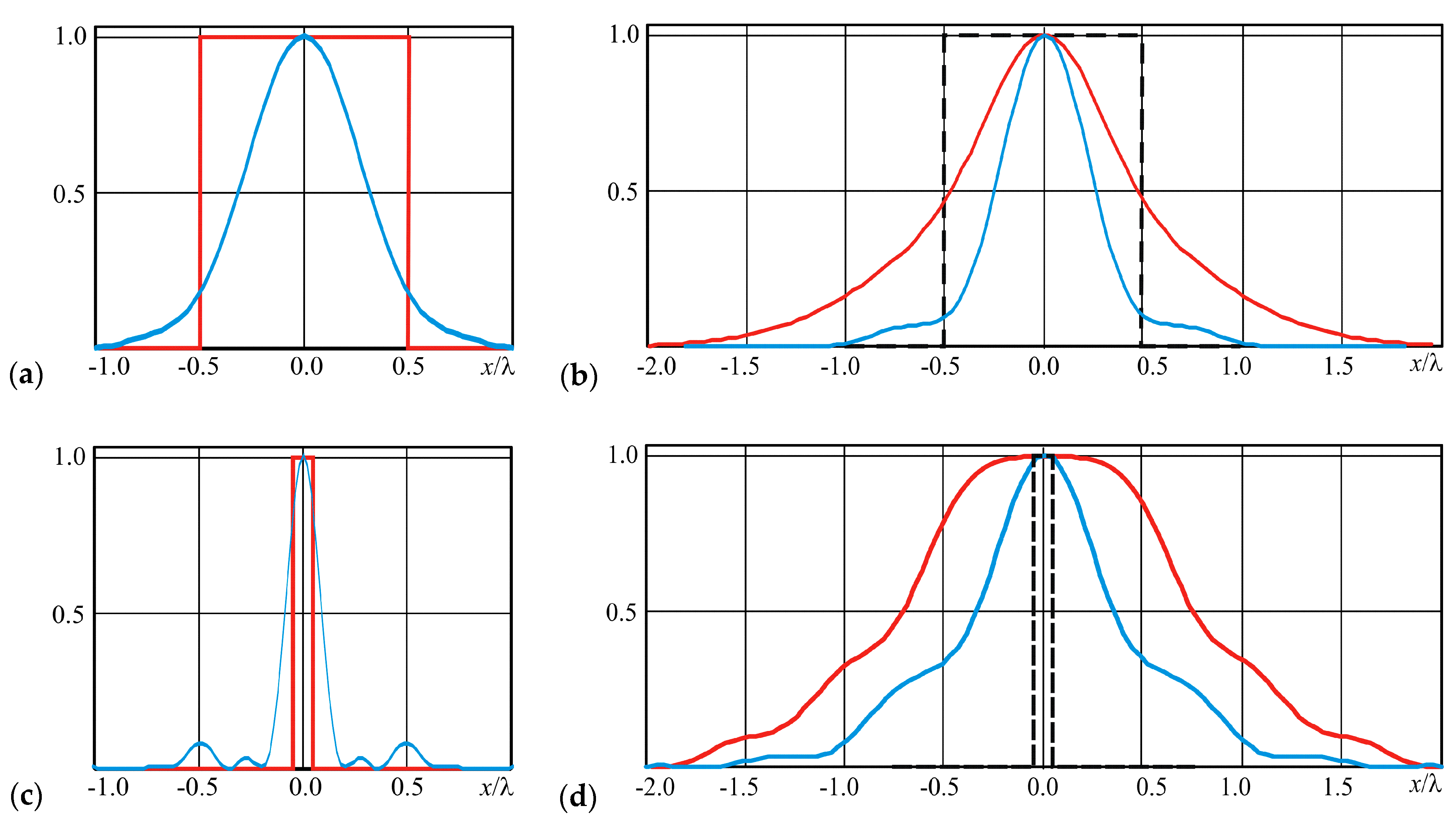
Let us consider the more general case of a superoscillating field, which was proposed by Berry and Popescu [23]:
f ( x ) = ( cos x + i a sin x ) N , ( a > 1 , N > > 1 ) ,
where a is a coefficient and N is a power degree. The influence of the parameters a and N on the form of the input field of Equation (6) is illustrated in Figure 6. It is seen that the coefficient a determines the period of the field, and the power degree N provides a high localization of energy at the maximum points.
Let us investigate the influence of the parameters a and N, as well as the size of the input field, on the possibility of overcoming the diffraction limit outside the region of evanescent waves (we define z = λ).
Initially, the parameters N = 20 and T = 5λ are fixed, and change the parameter a. Recall that in the definition of the function of Equation (6) a > 1 , N > > 1 . Accordingly, parameter a cannot be greater than the value of N. Therefore, condition a < N will be further considered.
The importance of parameter a from Figure 7 can be seen. An increase in value a makes it possible to form a compact light spot (the size of which is smaller than the diffraction limit) outside the near-field region. Note, however, that with an increase in parameter a > 10, the size of the central spot does not change, but there is a noticeable increase in the sidelobes.
It was shown in the previous section that the effect of the input field size T is important to overcome the diffraction limit. Therefore, let us find out the effect of this parameter for the field of Equation (6). The calculation results are shown in Figure 8. As can be seen, increasing the size of the input field T by 4 times slightly improved the situation. This is an important positive point since it is not always possible to significantly increase the size of the input field.
Let us also investigate the influence of the degree N on the possibility of light localization. From Figure 9, it can be seen that the positive effect of increasing the power degree N on decreasing the sidelobe level. However, with significant suppression of sidelobes, the broadening of the central peak occurs. A similar situation was observed with sharp focusing, which led to the need to search for a compromise between a decrease in the size of the light spot and an increase inside lobes [30,31]. In our case, the choice of the following parameters a = 10, N = 100, T = 5λ can be considered a compromise option. The results propagation simulation of such a field at various distances are shown in Figure 10.
As can be seen from the results shown in Figure 10, the field changes significantly during propagation. Although the size of the central spot remains below the diffraction limit, the level of the sidelobes changes significantly.
Thus, by varying the parameters of the superoscillating field of Equation (6), it is possible to overcome the diffraction limit with a reduced level of sidelobes, but only at a certain distance. Unfortunately, it is not possible to determine in advance at what distance the desired result will be achieved. This problem can be partially solved using an optimization algorithm. The possible approaches to solving the problem of overcoming the diffraction limit with the controlled growth of sidelobes are discussed in the next section.

4. Discussion

The problem of minimizing the focal spot with suppressed sidelobes is usually solved by apodizing the focusing system. As a rule, the lens is complemented by a filter that can be an amplitude element (mainly to stop illumination in the center of the pupil function) [35,36,37], a phase-only element (introducing phase modulation without energy absorption) [38,39,40,41,42], and, also, an amplitude–phase element (introducing both energy absorption and phase modulation) [31,43,44].
In Table 1, some results of a radially polarized beam that is tightly focused (numerical aperture of a lens with the radius R and the focal distance f  N A l e n s = sin [ arctg ( R / f ) ] was close to the highest value for free space 0.99) are discussed with different types of pupil function apodization [31]: full-aperture illumination (without apodization), a narrow annular aperture (amplitude apodization), and a ring aperture with phase jump. For a high NA focusing system, the propagation operator in Debye’s approximation [26,30,36,40,41,42] is used. To evaluate the sidelobe level S, the ratio of the intensity in the sidelobe to the intensity in the central spot is calculated.
As can be seen, the narrow annular aperture provides the minimum focal spot size (0.36λ is the diffraction limit for the Bessel beam [45,46]) almost without sidelobe growth (Table 1, line 2). However, this results in a significant loss of energy (the amplitude at the focus is proportional to the ring width [31]). To increase the energy efficiency without increasing the spot size, one can use amplitude–phase apodization—a wide ring with a phase jump (Table 1, line 3). In this case, a noticeable growth of sidelobes is observed.
Thus, reaching a trade-off between reducing the focal spot size, conserving energy, and suppressing sidelobes is a difficult task that requires the use of optimization algorithms. Different algorithms are known that make it possible to reduce the size of the focal spot with controlled growth of sidelobes [47,48]; however, as a rule, these algorithms do not provide high energy efficiency. The result of modeling using the algorithm described in [30] makes it possible to reduce the sidelobes below 30% while maintaining the minimum size of the focal spot due to some decrease in efficiency (Table 1, line 4).
These examples illustrate the competing nature of such parameters as the size of the focal spot, the amount of energy in the spot, and the level of sidelobes. Moreover, in the far diffraction zone (for example, in the focal region), it is difficult to significantly overcome the diffraction limit using simple types of pupil function apodization. Therefore, to significantly reduce the size of the light spot, diffraction in the near field is considered. For example, the results of the formation of a very compact light spot in the near field using the fractional axicon [11,49] are shown in Figure 11. As can be seen, at distance z = 0.01λ, the formation of a central spot with a size much less than the diffraction limit is possible: FWHM = 0.123λ (Figure 11a) and FWHM = 0.118λ (Figure 11b). Note, outside the zone of evanescent waves, the central spot broadens significantly: FWHM = 0.395λ (Figure 11a) and FWHM = 0.4λ (Figure 11b).
One of the approaches to reduce the spreading of a light spot during propagation is based on the signal approximation by the eigenfunctions of an optical system [34,50,51,52,53,54,55]. The most famous are spheroidal functions representing the eigenfunctions of the bounded Fourier operator [56,57,58,59]. When using several lenses, as well as for more complex optical systems, the eigenfunctions are calculated numerically [60,61].
In Figure 12, the results of the generation of a compact light spot based on approximation of the input rectangle signal by eigenfunctions of the free-space propagation operator (4) with the spectral domain bounded by the interval of spatial frequencies | α 0 | < 1.5 are shown. The results for the rectangular signals are shown in red color, and the results for the corresponding approximations are shown in blue color. It can be seen that the approximation of a signal whose width is 1λ (Figure 12a,b) does not broaden when propagating to a distance of z = λ: the size of the approximation in the input plane is FWHM = 0.64λ (Figure 12a), and at the distance z = λ FWHM = 0.57λ (Figure 12b). If the input signal has a width significantly less than the diffraction limit, in particular, 0.1λ (Figure 12c,d), then the approximation broadens noticeably: the size of the approximation in the input plane is FWHM = 0.17λ (Figure 12c), and at the distance z = λ FWHM = 0.65λ (Figure 12d). This effect is associated with fundamental limitations of the resolution of the used optical system [62,63]. Note, however, that the use of an approximation based on eigenfunctions made it possible to significantly reduce the broadening of the original signal.
This discussion clearly showed the competing nature of parameters, such as the size of the focal spot and the level of sidelobes. The use of an optimizing algorithm provides a compromise solution to this problem, but only within the resolution of the optical system under consideration.

5. Conclusions

In this work, we studied and simulated the propagation of one-dimensional superoscillating signals of two types: based on the superposition of spatial harmonics and based on the power of the complex function. To simulate the propagation of superoscillating fields, an operator was used based on the plane waves expansion.
The results of comparative modeling showed that the first type of superoscillating function, which is a superposition of spatial harmonics, ensures that the diffraction limit is overcome over an extended distance if the size of the input field is several tens of wavelengths. In this case, however, in the generated distributions, the central peak is too closely surrounded by sidelobes of approximately the same height. The use of such distributions is problematic even in scanning optical systems.
Another type of superoscillating signal, which is a power-law function of the complex harmonics, makes it possible to overcome the diffraction limit with a reduced level of sidelobes at a certain distance outside the zone of evanescent waves. This requires the selection of the parameters of the superoscillating field, and it is not possible to determine in advance at what distance the desired result will be achieved. This problem can be partially solved using an optimization algorithm. In this case, it is important to know the influence of each parameter, which makes the performed studies useful. In particular, it was shown that spatial frequencies bounding by the value α 0 = 1.5 is suitable if the propagation of the field outside the region of evanescent waves is considered.
A discussion of various approaches to solving the problem of minimizing the focal spot with suppressed sidelobes revealed the competing nature of such parameters as the size of the focal spot and the level of sidelobes. The use of an optimizing algorithm provides a compromise solution to this problem, but only within the framework of the resolution of the optical system under consideration, which can be estimated based on the calculation of the eigenfunctions of the system.

Author Contributions

Conceptualization, S.N.K., E.D.P., and M.A.B.; methodology, S.N.K., E.D.P., and M.A.B.; software, S.N.K., E.D.P., and M.A.B.; validation, S.N.K., E.D.P., and M.A.B.; formal analysis, S.N.K., E.D.P., and M.A.B.; investigation, S.N.K., E.D.P., and M.A.B.; resources, S.N.K., E.D.P., and M.A.B.; data curation, S.N.K., E.D.P., and M.A.B.; writing—original draft preparation, S.N.K., E.D.P., and M.A.B.; writing—review and editing, S.N.K., E.D.P., and M.A.B.; visualization, S.N.K., E.D.P., and M.A.B.; supervision, S.N.K., E.D.P., and M.A.B.; project administration, S.N.K., E.D.P., and M.A.B.; funding acquisition, S.N.K., E.D.P., and M.A.B. All authors have read and agreed to the published version of the manuscript.

Funding

This work was financially supported by the Russian Foundation for Basic Research under grant No. 18-07-01470 (numerical calculations), by the Ministry of Science and Higher Education within the State assignment to the FSRC «Crystallography and Photonics» RAS No. 007-GZ/Ch3363/26 (theoretical research) and under the Samara National Research University within the scientific state assignment No. 0777-2020-0017 (comparative analysis).

Institutional Review Board Statement

Not applicable.

Informed Consent Statement

Not applicable.

Data Availability Statement

Not applicable.

Acknowledgments

We acknowledge the equal contribution of all the authors.

Conflicts of Interest

The authors declare no conflict of interest.

References

  1. Rayleigh, L. On the theory of optical images with special reference to the optical microscope. Philos. Mag. 1896, 5, 167–195. [Google Scholar] [CrossRef] [Green Version]
  2. Betzig, E.; Trautman, J.K.; Harris, T.D.; Weiner, J.S.; Kostelak, R.L. Breaking the diffraction barrier: Optical microscopy on a nanometric scale. Science 1991, 251, 1468–1470. [Google Scholar] [CrossRef] [PubMed]
  3. Betzig, E.; Trautman, J.K. Near-field optics: Microscopy, spectroscopy, and surface modification beyond the diffraction limit. Science 1992, 257, 189–195. [Google Scholar] [CrossRef] [Green Version]
  4. Heinzelmann, H.; Pohl, D. Scanning near-field optical microscopy. Appl. Phys. A 1994, 59, 89–101. [Google Scholar] [CrossRef]
  5. Girard, C.; Dereux, A. Near-field optics theories. Rep. Prog. Phys. 1996, 59, 657–699. [Google Scholar] [CrossRef] [Green Version]
  6. Hecht, B.; Sick, B.; Wild, U.P.; Deckert, V.; Zenobi, R.; Martin, O.J.F.; Pohl, D.W. Scanning near-field optical microscopy with aperture probes: Fundamentals and applications. J. Chem. Phys. 2000, 112, 7761–7774. [Google Scholar] [CrossRef]
  7. De Serio, M.; Zenobi, R.; Deckert, V. Looking at the nanoscale: Scanning near-field optical microscopy. TrAC Trend. Anal. Chem. 2003, 22, 70–77. [Google Scholar] [CrossRef]
  8. Shifa, W. Review of near field microscopy. Front. Phys. Chin. 2006, 1, 263–274. [Google Scholar]
  9. Lereu, A.; Passian, A.; Dumas, P. Near-field optical microscopy: A brief review. Int. J. Nanotechnol. 2012, 9, 3–7. [Google Scholar] [CrossRef]
  10. Degtyarev, S.A.; Khonina, S.N. Transmission of focused light signal through an apertured probe of a near-field scanning microscope. Pattern Recognit. Image Anal. 2015, 25, 306–313. [Google Scholar] [CrossRef]
  11. Khonina, S.N.; Ustinov, A.V. Very compact focal spot in the near-field of the fractional axicon. Opt. Commun. 2017, 391, 24–29. [Google Scholar] [CrossRef]
  12. Bazylewski, P.; Ezugwu, S.; Fanchini, G. A review of three-dimensional scanning near-field optical microscopy (3D-SNOM) and its applications in nanoscale light management. Appl. Sci. 2017, 7, 973. [Google Scholar] [CrossRef] [Green Version]
  13. Kowarz, M.W. Homogeneous and evanescent contributions in scalar near-field diffraction. Appl. Opt. 1995, 34, 3055–3063. [Google Scholar] [CrossRef] [PubMed]
  14. Katrich, A.B. Do evanescent waves really exist in free space? Opt. Commun. 2005, 255, 169–174. [Google Scholar] [CrossRef]
  15. Rasmussen, A.; Deckert, V. New dimension in nano-imaging:breaking through the diffraction limit with scanning near-field optical microscopy. Anal. Bioanal. Chem. 2005, 381, 165–172. [Google Scholar] [CrossRef]
  16. Rotenberg, N.; Kuipers, L. Mapping nanoscale light fields. Nat. Photonics 2014, 8, 919–926. [Google Scholar] [CrossRef]
  17. Degtyarev, S.A.; Ustinov, A.V.; Khonina, S.N. Nanofocusing by sharp edges. Comput. Opt. 2014, 38, 629–637. [Google Scholar] [CrossRef] [Green Version]
  18. Gramotnev, D.K.; Bozhevolnyi, S.A. Nanofocusing of electromagnetic radiation. Nat. Photonics 2014, 8, 13–22. [Google Scholar] [CrossRef]
  19. Degtyarev, S.A.; Porfirev, A.P.; Ustinov, A.V.; Khonina, S.N. Singular laser beams nanofocusing with dielectric nanostructures: Theoretical investigation. J. Opt. Soc. Am. B 2016, 33, 2480–2485. [Google Scholar] [CrossRef]
  20. Di Francia, G.T. Super-gain antennas and optical resolving power. Il Nuovo Cimento 1952, 9, 426–438. [Google Scholar] [CrossRef]
  21. Bucklew, J.A.; Saleh, B.E.A. Theorem for high-resolution high-contrast image synthesis. J. Opt. Soc. Am. A 1985, 2, 1233–1236. [Google Scholar] [CrossRef]
  22. Aharonov, Y.; Albert, D.Z.; Vaidman, L. How the result of a measurement of a component of the spin of a spin-1/2 particle can turn out to be 100. Am. Phys. Soc. 1988, 60, 1351–1354. [Google Scholar]
  23. Berry, M.V.; Popescu, S. Evolution of quantum superoscillations and optical superresolution without evanescent waves. J. Phys. A 2006, 39, 6965–6977. [Google Scholar] [CrossRef]
  24. Ferreira, P.J.S.G.; Kempf, A. Superoscillations: Faster than the Nyquist rate. IEEE Trans. Signal Process. 2006, 54, 3732–3740. [Google Scholar] [CrossRef] [Green Version]
  25. Huang, F.M.; Zheludev, N.I. Super-resolution without evanescent waves. Nano Lett. 2009, 9, 1249–1254. [Google Scholar] [CrossRef] [Green Version]
  26. Kant, R. Superresolution and increased depth of focus:an inverse problem of vector diffraction. J. Mod. Opt. 2000, 47, 905–916. [Google Scholar] [CrossRef]
  27. Rao, R.; Mitic, J.; Serov, A.; Leitgeb, R.A.; Lasser, T. Field confinement with aberration correction for solid immersion lens based fluorescence correlation spectroscopy. Opt. Commun. 2007, 271, 462–469. [Google Scholar] [CrossRef]
  28. Khonina, S.N.; Nesterenko, D.V.; Morozov, A.A.; Skidanov, R.V.; Soifer, V.A. Narrowing of a light spot at diffraction of linearly-polarized beam on binary asymmetric axicons. Opt. Mem. Neural Netw. 2012, 21, 17–26. [Google Scholar] [CrossRef]
  29. Hyvarinen, H.J.; Rehman, S.; Tervo, J.; Turunen, J.; Sheppard, C.J.R. Limitations of superoscillation filters in microscopy applications. Opt. Lett. 2012, 37, 903–905. [Google Scholar] [CrossRef]
  30. Khonina, S.N.; Volotovskiy, S.G. Minimizing the bright/shadow focal spot size with controlled side-lobe increase in high-numerical-aperture focusing systems. Adv. Opt. Technol. 2013, 2013, 267684. [Google Scholar] [CrossRef] [Green Version]
  31. Khonina, S.N.; Ustinov, A.V. Sharper focal spot for a radially polarized beam using ring aperture with phase jump. J. Eng. 2013, 2013, 512971. [Google Scholar] [CrossRef] [Green Version]
  32. Huang, F.M.; Chen, Y.; De Abajo, F.J.G.; Zheludev, N.I. Optical super-resolution through super-oscillations. J. Opt. A Pure Appl. Opt. 2007, 9, S285. [Google Scholar] [CrossRef]
  33. Khonina, S.N.; Ustinov, A.V.; Kovalyov, A.A.; Volotovsky, S.G. Near-field propagation of vortex beams: Models and computation algorithms. Opt. Mem. Neural Netw. 2014, 23, 50–73. [Google Scholar] [CrossRef]
  34. Khonina, S.N.; Kirilenko, M.S.; Volotovsky, S.G. Defined distribution forming in the near diffraction zone based on expansion of finite propagation operator eigenfunctions. Procedia Eng. 2017, 201, 53–60. [Google Scholar] [CrossRef]
  35. Boivin, R.; Boivin, A. Optimized amplitude filtering for superresolution over a restricted field: I. Achievement of maximum central irradiance under an energy constraint. Opt. Acta 1980, 27, 587–610. [Google Scholar]
  36. Quabis, S.; Dorn, R.; Eberler, M.; Glöckl, O.; Leuchs, G. Focusing light to tighter spot. Opt. Commun. 2000, 179, 1–7. [Google Scholar] [CrossRef]
  37. Reddy, A.N.K.; Khonina, S.N. Apodization for improving the two-point resolution of coherent optical systems with defect of focus. Appl. Phys. B 2018, 124, 229. [Google Scholar] [CrossRef]
  38. Sales, T.R.M.; Morris, G.M. Diffractive superresolution elements. J. Opt. Soc. Am. A 1997, 14, 1637–1646. [Google Scholar] [CrossRef]
  39. de Juana, D.M.; Oti, J.E.; Canales, V.F.; Cagigal, M.P. Design of superresolving continuous phase filters. Opt. Lett. 2003, 28, 607–609. [Google Scholar] [CrossRef]
  40. Sheppard, C.J.R. Filter performance parameters for high-aperture focusing. Opt. Lett. 2007, 32, 1653–1655. [Google Scholar] [CrossRef]
  41. Khonina, S.N.; Ustinov, A.V.; Pelevina, E.A. Analysis of wave aberration influence on reducing focal spot size in a high-aperture focusing system. J. Opt. 2011, 13, 095702. [Google Scholar] [CrossRef]
  42. Khonina, S.N. Simple phase optical elements for narrowing of a focal spot in high-numerical-aperture conditions. Opt. Eng. 2013, 52, 091711. [Google Scholar] [CrossRef]
  43. Ledesma, S.; Campos, J.; Escalera, J.C. Simple expressions for performance parameters of complex filters, with application to super-Gaussian phase filters. Opt. Lett. 2004, 29, 932–934. [Google Scholar] [CrossRef] [Green Version]
  44. Chen, J.; Kuang, D.-F.; Fang, Z.-L. Properties of Fraunhofer Diffraction by an Annular Spiral Phase Plate for Sidelobe Suppression. Chin. Phys. Lett. 2009, 26, 094210. [Google Scholar]
  45. Kalosha, V.P.; Golub, I. Toward the subdiffraction focusing limit of optical superresolution. Opt. Lett. 2007, 32, 3540–3542. [Google Scholar] [CrossRef]
  46. Khonina, S.N.; Kazanskiy, N.L.; Karpeev, S.V.; Butt, M.A. Bessel Beam: Significance and Applications—A Progressive Review. Micromachines 2020, 11, 997. [Google Scholar] [CrossRef]
  47. Cagigal, M.P.; Oti, J.E.; Canales, V.F.; Valle, P.J. Analytical design of superresolving phase filters. Opt. Commun. 2004, 241, 249–253. [Google Scholar] [CrossRef]
  48. Liu, H.; Yan, Y.; Jin, G. Design theories and performance limits of diffractive superresolution elements with the highest sidelobe suppressed. J. Opt. Soc. Am. A 2005, 22, 828–838. [Google Scholar] [CrossRef]
  49. Ustinov, A.V.; Khonina, S.N. Fracxicon as hybrid element between the parabolic lens and the linear axicon. Comput. Opt. 2014, 38, 402–411. [Google Scholar] [CrossRef]
  50. Pierri, R.; Soldovieri, F. On the information content of the radiated fields in the near zone over bounded domains. Inverse Probl. 1998, 14, 321–337. [Google Scholar] [CrossRef]
  51. Miller, D.A.B. Communicating with waves between volumes: Evaluating orthogonal spatial channels and limits on coupling strengths. Appl. Opt. 2000, 39, 1681–1699. [Google Scholar] [CrossRef] [Green Version]
  52. Thaning, A.; Martinsson, P.; Karelin, M.; Friberg, A.T. Limits of diffractive optics by communication modes. J. Opt. A Pure Appl. Opt. 2003, 5, 153–158. [Google Scholar] [CrossRef]
  53. Mazilu, M.; Baumgartl, J.; Kosmeier, S.; Dholakia, K. Optical Eigenmodes; exploiting the quadratic nature of the energy flux and of scattering interactions. Opt. Express 2011, 19, 933–945. [Google Scholar] [CrossRef] [Green Version]
  54. Baumgartl, J.; Kosmeier, S.; Mazilu, M.; Rogers, E.T.F.; Zheludev, N.I.; Dholakia, K. Far field subwavelength focusing using optical eigenmodes. Appl. Phys. Lett. 2011, 98, 181109. [Google Scholar] [CrossRef] [Green Version]
  55. Kirilenko, M.S.; Khonina, S.N. Formation of signals matched with vortex eigenfunctions of bounded double lens system. Opt. Commun. 2018, 410, 153–159. [Google Scholar] [CrossRef]
  56. Slepian, D.; Pollak, H.O. Prolate spheroidal wave functions, Fourier analysis and uncertainty—I. Bell Syst. Technol. J. 1961, 40, 43–63. [Google Scholar] [CrossRef]
  57. Landau, H.J.; Pollak, H.O. Prolate spheroidal wave functions, Fourier analysis and uncertainty—II. Bell Syst. Technol. J. 1961, 40, 65–84. [Google Scholar] [CrossRef]
  58. Khonina, S.N.; Volotovskii, S.G.; Soifer, V.A. A method for computing the eigenvalues of prolate spheroidal functions of order zero. Dokl. Math. 2001, 63, 136–138. [Google Scholar]
  59. Karoui, A.; Moumni, T. Spectral analysis of the finite Hankel transform and circular prolate spheroidal wave functions. J. Comput. Appl. Math. 2009, 233, 315–333. [Google Scholar] [CrossRef] [Green Version]
  60. Kirilenko, M.S.; Zubtsov, R.O.; Khonina, S.N. Calculation of eigenfunctions of a bounded fractional Fourier transform. Comput. Opt. 2015, 39, 332–338. [Google Scholar] [CrossRef] [Green Version]
  61. Kirilenko, M.S.; Zubtsov, R.O.; Khonina, S.N. Calculation of eigenfunctions of bounded waveguide with quadratic refractive index. J. Phys. Conf. Ser. 2016, 735, 012002. [Google Scholar] [CrossRef] [Green Version]
  62. Gallager, R.G. Information Theory and Reliable Communication; John Wiley & Sons, Inc.: New York, NY, USA, 1968; ISBN 978-0-471-29048-3. [Google Scholar]
  63. Di Francia, G.T. Degrees of freedom of an image. J. Opt. Soc. Am. 1969, 59, 799–804. [Google Scholar] [CrossRef] [PubMed]
Figure 1. Superoscillating signal of Equation (1).
Optics 02 00015 g001
Figure 2. Features of the superoscillating field: comparative distributions for the functions of Equation (1)—bold line, Equation (2)—dashed line, and of Equation (3)—thin line.
Optics 02 00015 g002
Figure 3. The spatial spectrum of the field of Equation (1): (a) initial and (b) truncated following function of Equation (5).
Optics 02 00015 g003
Figure 4. Field of Equation (4) at the distance z = 0.5λ.
Optics 02 00015 g004
Figure 5. Field amplitude of Equation (1) propagated at the distance (a) z = 1.5λ, (b) z = 7λ, (c) z = 15λ, (d) z = 100λ.
Optics 02 00015 g005
Figure 6. Complex field distribution of Equation (6) for a = 2 at different values of the power degree: (a) N = 2, (b) N = 5, (c) N = 10, (d) N = 100 (the amplitude is shown by the solid line, and the phase by the dashed line).
Optics 02 00015 g006
Figure 7. Amplitude of the field of Equation (6) at a distance z = λ for N = 20 and T = 5λ at different values of the coefficient: (a) a = 1.5, (b) a = 5, (c) a = 10, (d) a = 20.
Optics 02 00015 g007
Figure 8. The amplitude of the field of Equation (6) with a = 10 and N = 20 propagated at the distance z = λ for different sizes of the input field: (a) T = 2.5, (b) T = 10.
Optics 02 00015 g008
Figure 9. The amplitude of the field of Equation (6) with a = 10 and T = 5λ propagated at the distance z = λ for different values of the power degree: (a) N = 50, (b) N = 100, (c) N = 200, (d) N = 300.
Optics 02 00015 g009
Figure 10. The amplitude of the field of Equation (6) with a = 10, N = 100 and T = 5λ propagated at the different distances: (a) z = 0.5λ, (b) z = 0.8λ, (c) z = 3λ, (d) z = 4λ, (e) z = 5λ, (f) z = 6λ.
Optics 02 00015 g010
Figure 11. Generation of a compact light spot in the near-field zone by the fractional axicon τ ( r ) = exp [ i ( k α 0 r ) γ ] with (a) γ = 0.5, α 0 = 125 and (b) γ = 0.25, α 0 = 7937607 : graphs show normalized intensity sections at distance of z = 0.01λ (solid line), z = 0.1λ (dashed line), and z = 2λ (dotted line).
Optics 02 00015 g011
Figure 12. Generation of a compact light based on approximation of the input rectangle signal by eigenfunctions of the finite propagation operator (red color for the signal and blue color for an approximation): input signals of (a) 1λ and (c) 0.1λ width and corresponding diffraction results at z = λ distance (b,d), accordingly.
Optics 02 00015 g012
Table 1. Comparing results for a tightly focused radially polarized beam with different types of pupil function apodization (S is the sidelobe level).
Apodization (Amplitude and Phase Distribution)Distribution in the Focal Plane
(Intensity and Graph of Cross-Section)
Without apodization
Optics 02 00015 i001
Optics 02 00015 i002
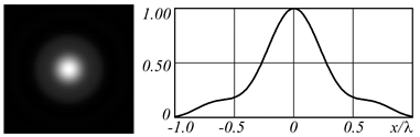
FWHM = 0.544λ, S = 0.16
Narrow ring
Optics 02 00015 i003
Optics 02 00015 i004
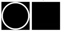
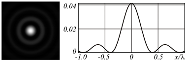
FWHM = 0.378λ, S = 0.162
Ring with phase jump
Optics 02 00015 i005
Optics 02 00015 i006
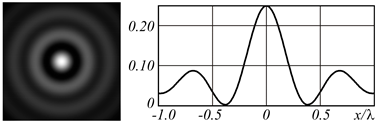
FWHM = 0.371λ, S = 0.351
Optimized function
Optics 02 00015 i007
Optics 02 00015 i008
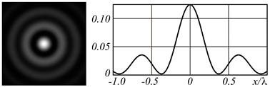
FWHM = 0.359λ, S = 0.28
Publisher’s Note: MDPI stays neutral with regard to jurisdictional claims in published maps and institutional affiliations.

