5.1. PIV Velocity Measurements
Figure 7 shows the resulting velocity fields of the PIV measurements with the flow in the cold layer of the stratification (
Figure 7a), in the height of the thermocline (
Figure 7b) and in the hot layer (
Figure 7c) [
27]. The surface of the aluminium wall is at the position
with
. The vector arrows show the flow field with a contour plot of the vertical velocity component in the background. The cell has been filled separately for each flow field, and PIV measurements have been started five minutes after the end of filling. Preliminary, qualitative investigations have shown that this time is sufficient to allow the inlet flow in the bottom to settle down and that, at the same time, it is short enough that the high degree of thermal stratification from the beginning of the stand-by period to be still present.
Inlet temperatures of each measurement have been in a range from 58 to for hot layers and between 6 and for cold layers. The water temperatures measured inside the cell have been between 52 and in the hot layer and 9 and in the cold layer for all measurements. Changes in water temperature during the filling have occurred as the cell has to adopt the temperature of the water. Thus, the cell heats or cools the water, respectively. Differences in the measured stratification temperatures may result from different room temperatures as the measurements have not been performed at the same day. However, the typical flow features and characteristic curves that this study deals with are not significantly affected by small temperature differences between the measurements.
The evaluation of the flow fields in
Figure 7a,b have been made by averaging 499 vector fields of 500 raw images with a time difference of
resulting in an overall time average of
. The resolution of the calculated vectors is
which converts together with an overlap of 50% of the vectors to
.
Figure 7c shows an averaged vector field of 9000 images with the same difference in time of
. The higher number of images used for the averaging is a result of fluctuations that have occurred in this region so that more time steps have been needed. As mentioned in the discussion of
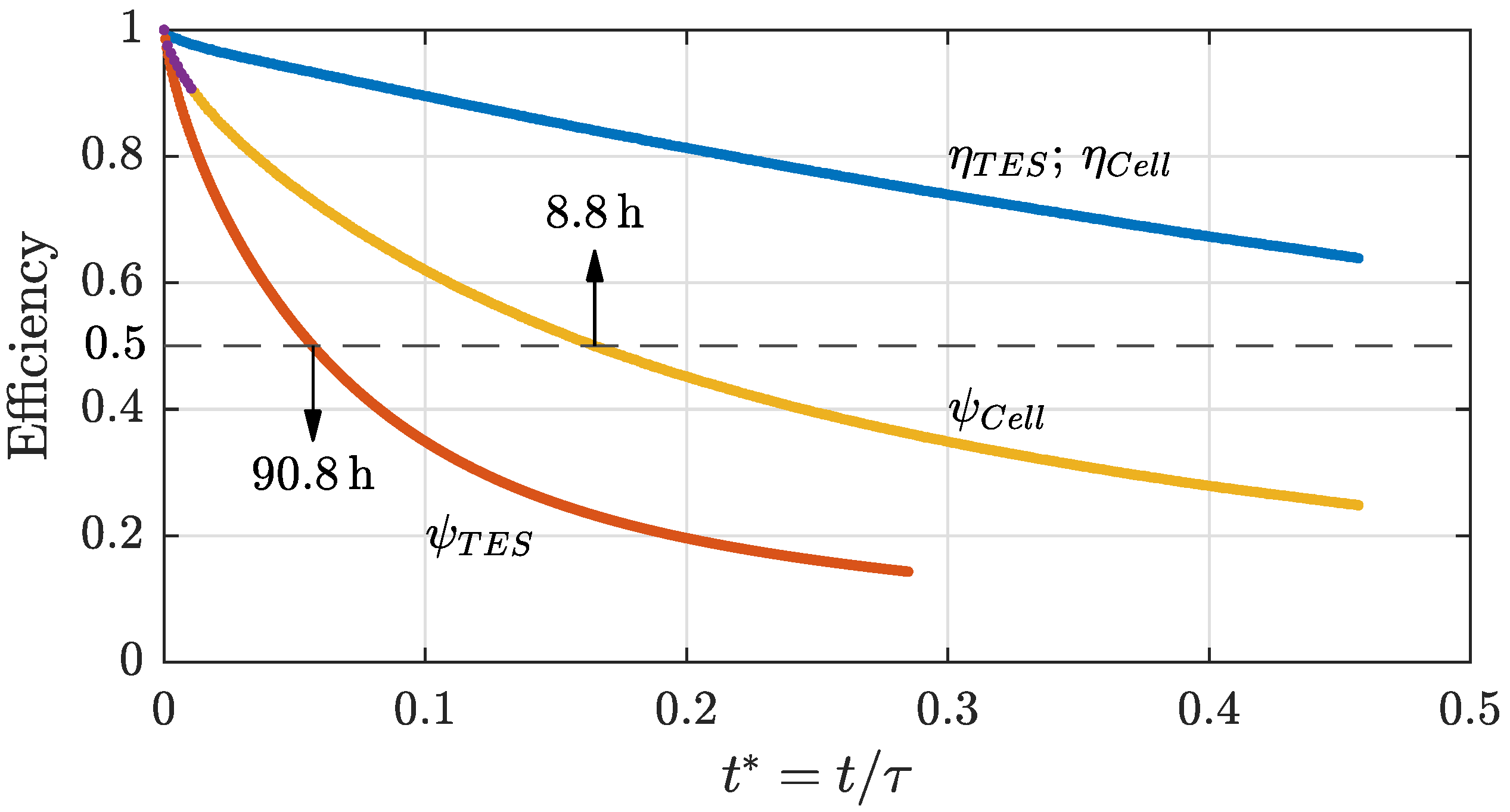
Figure 4, the whole process is transient. Therefore, the state of the experiment at the beginning of the measurement time is another than in the end. However, the violet part of the cell’s exergy efficiency curve shows that during the measurement time, the exergy efficiency decreases about only 10%. With the objective of this measurement to get a general impression of the flow, this change is small enough not to affect the result.
The basis of the averaging in
Figure 7c are vector fields that have been calculated using the pyramid sum of correlation algorithm with Gaussian weighting [
28]. This algorithm uses the correlation of not only two consecutive raw images but takes correlations of every possible combination of a range of three or more images into consideration. Therefore, low, as well as high velocities, can be evaluated at the same time, and velocity gradients can be resolved better by the cost of temporal resolution. In this case, a range of five raw images has been used to calculate one quasi-instantaneous flow field. Therefore the time averaging for one single vector field was
. The spatial resolution can be increased [
29], resulting in a resolution of one vector of
which corresponds, with an overlap of 50% of each vector, to
.
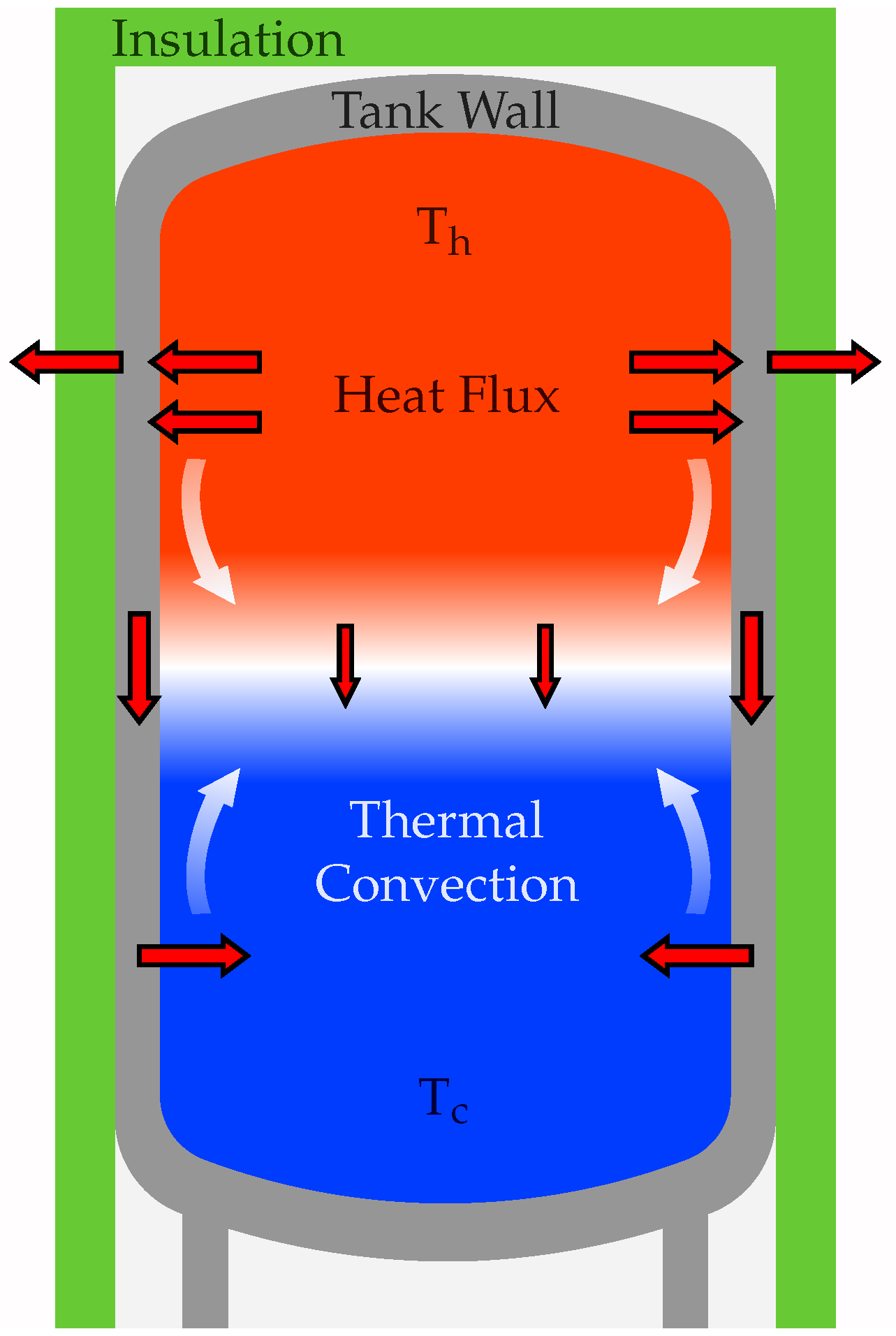
The time-averaged flow fields show two vertical wall jets, one in the hot and one in the cold layer of the stratification. The downward-directed jet in the upper part results from the heat flux that heats the aluminium wall and cools the water in this region and the upward-directed jet in the lower part is a result of the cold water which gets heated by the aluminium wall in this region. The two counter-directed wall jets approach at
in the region of the thermocline which can be seen in
Figure 7b. The collision slows down the wall jets and creates a relatively weak horizontal flow towards the centre of the measuring cell. The horizontal velocities of this flow are one to two orders of magnitude lower than the vertical velocities in the wall jets at this height as the flow spreads over a broader region as in the wall jets.
Comparison of
Figure 7b with
Figure 7a,c shows that the velocities of the wall jets increases with greater distance to the centre of the thermocline. The maximum of their thickness does not seem to be reached in the regions shown since both jets widen continuously in the areas of the
Figure 7b,c. Further comparison of the two wall jets with one another shows that the upward-directed jet is thicker but slower than the downward-directed jet. This behaviour is plausible taking into account the kinematic viscosity of water which differs from
for the cold temperature of
and
for the hot temperature of
resulting in a change of 57% [
30]. The higher viscosity in the cold layer leads to a thicker wall jet because of the higher friction in the fluid. Furthermore, the lower viscosity in the upper part favours higher velocities and a thinner wall jet at the same time. As indicated earlier, there are more fluctuations in the velocity field in the upper part, which made averaging over more individual time steps necessary to obtain the velocity field in
Figure 7c. These fluctuations are investigated in more detail in the following.
For this reason, time-series data of the vertical velocity component
as well as its normalised temporal development
has been analysed at three points in space where each of them is in the middle of one of the investigated three measurement areas. The results are shown in
Figure 8. The vertical positions of the three points are
as shown in the legend of diagram
Figure 8a. The horizontal positions of the points have been chosen to be
away from the wall surface which equals
as this is still inside the field of view but at the same time outside of the wall jets of the time-averaged flow fields. In this position, the velocity should be steady and near to zero in the case of laminar flow. Otherwise, fluctuations occur that can be analysed to get a deeper understanding of the flow characteristics.
Figure 8a shows that the flow in the bottom at
and in the thermocline at
seems to be laminar because both of the time-series stay nearly constant over the entire period of
. In the cold region at a height of
the measured vertical velocity is with an averaged value of
negative compared to that in the thermocline at
with
. The negative velocity shows that outside of the wall jet, a counter-directed shear flow is existent, which can be explained by the inertia of the fluid. A small fluid portion that flows with the wall jet upwards indeed reaches the height where it has the same density as stratification in this height, but due to its inertia, it is flowing beyond this position. Therefore, the buoyancy force acting on the fluid portion changes its sign so that the fluid has to flow back, which results in the shear flow. In the thermocline, both wall jets approach and thus a shear flow is not existent in this area.
The vertical velocity component in the hot part of the stratification shows a completely different behaviour than in the other parts of the cell. It constantly changes and thereby varies between a minimum velocity of to a maximum of . The difference between the velocities in the hot and cold layer is due to the temperature dependant properties of water, as stated before.
Figure 8b shows the same time-series as before but normalised by their maximum values. It is noticeable that the relative fluctuations in the thermocline are nearly as high as in the hot region shown in their standard deviations of
and
, respectively. In comparison to that, the normalised velocity in the bottom region of the measuring cell is still nearly constant with a standard deviation of only
. In contrast to the signal of the hot part, the velocities in the thermocline and the bottom are much more covered by noise. This is since the relative uncertainty of PIV measurements is higher for lower velocities as the particle shift between the images is shorter while the accuracy of the position determination remains the same with about
[
23]. Most of the fluctuations in the bottom region can be attributed to this noise. In contrast, the velocity in the thermocline undergoes, additionally to the noise, significant changes that cannot be seen in
Figure 8a. As a result, the normalised time-series of the velocity shows that the fluctuations, which emerge in the wall jet of the hot layer, spread to the thermocline. There, they seem to decay as their influence is not noticeable in the cold part of the stratification.
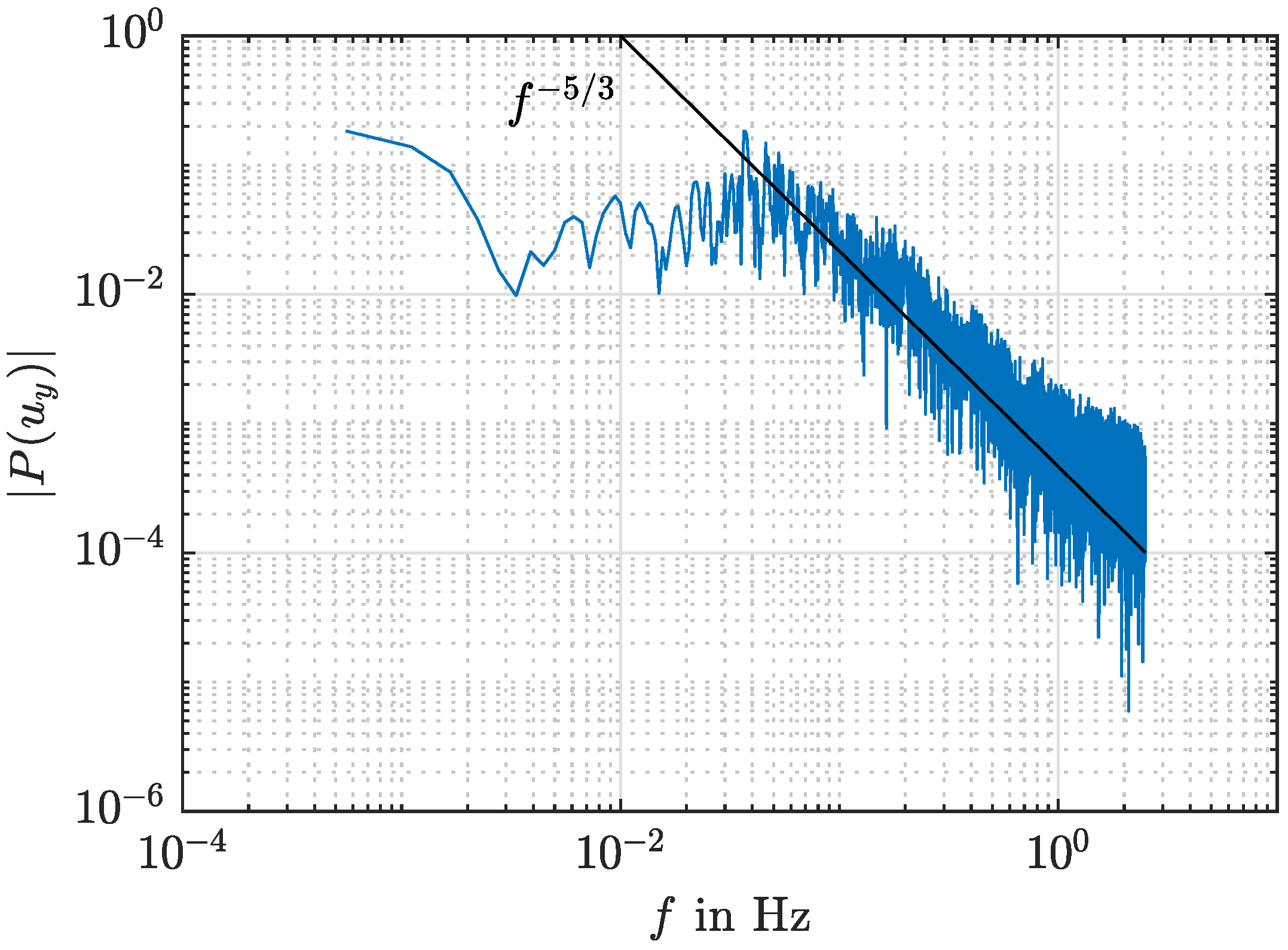
As a last step the amplitude spectrum
of the vertical velocity at
has been calculated, to check whether there is any kind of periodicity in the flow. For this reason, the whole data set of 9000 raw images has been used, corresponding to a period of 1800 s. Significant periodic features of the flow would result in an outstanding peak of the spectrum.
Figure 9 shows the results of the amplitude spectrum in a logarithmic scale. Starting at the lowest frequency the spectrum stays nearly constant with values in the range of
, and starts to decay with a nearly linear slope (in the logarithmic scale) from a frequency of about
. During this decay no significant peak in the spectrum can be recognised and therefore the flow in this region seems not to have a dominant periodic frequency. However, the spectrum is during its decrease parallel to
, and thus it follows the typical behaviour of turbulent motion described by Kolomogorovs
-law. The law describes the fact that large vortices in turbulent motion disintegrate into smaller ones until their kinetic energy transfers into heat due to viscosity. In future investigations the vortices in the fluctuating flow in the upper part of the cell will be investigated more precisely. Furthermore, it can be assumed that the flow is not only two-dimensional but has a third component, which can be measured in the future by stereoscopic or tomographic PIV investigations.
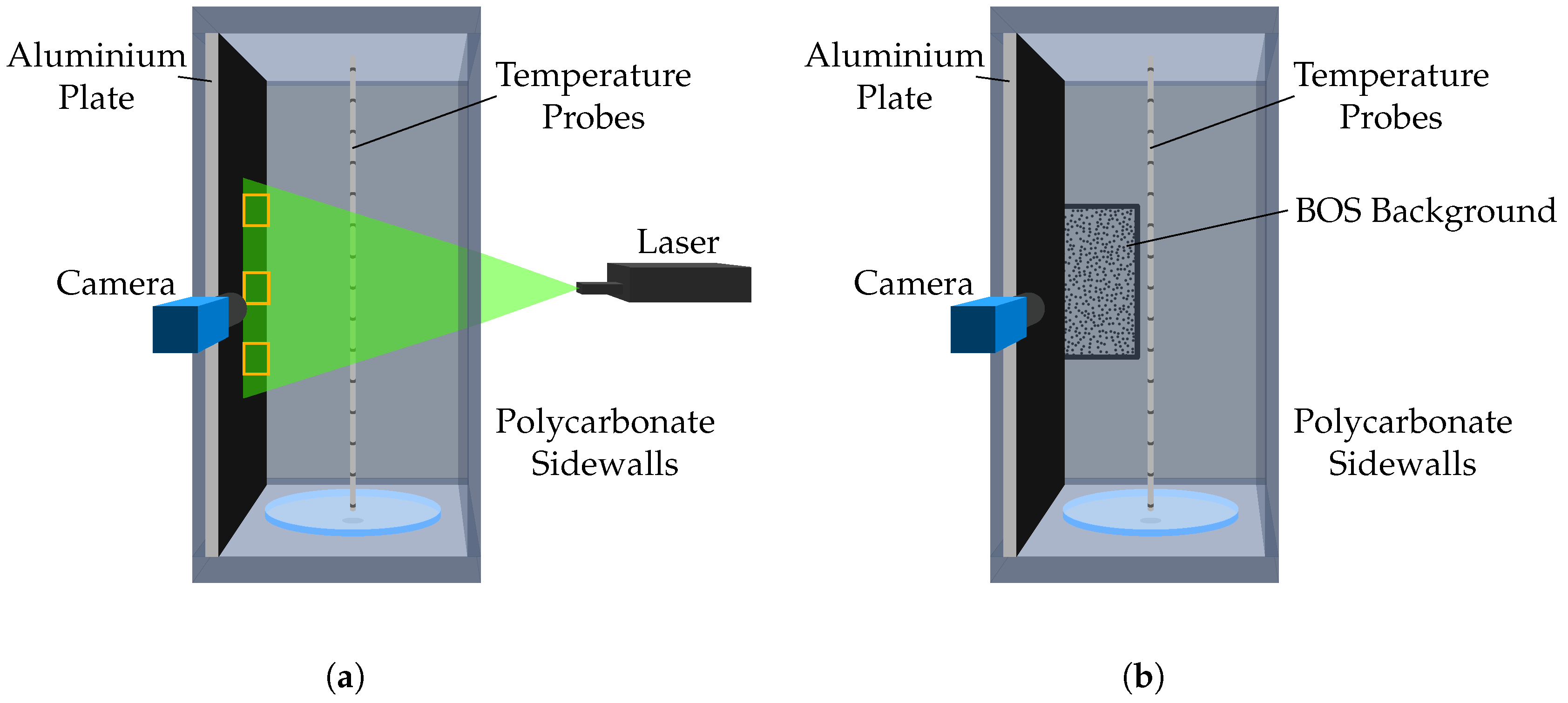
5.2. Temperature Field Measurements with the BOS Method
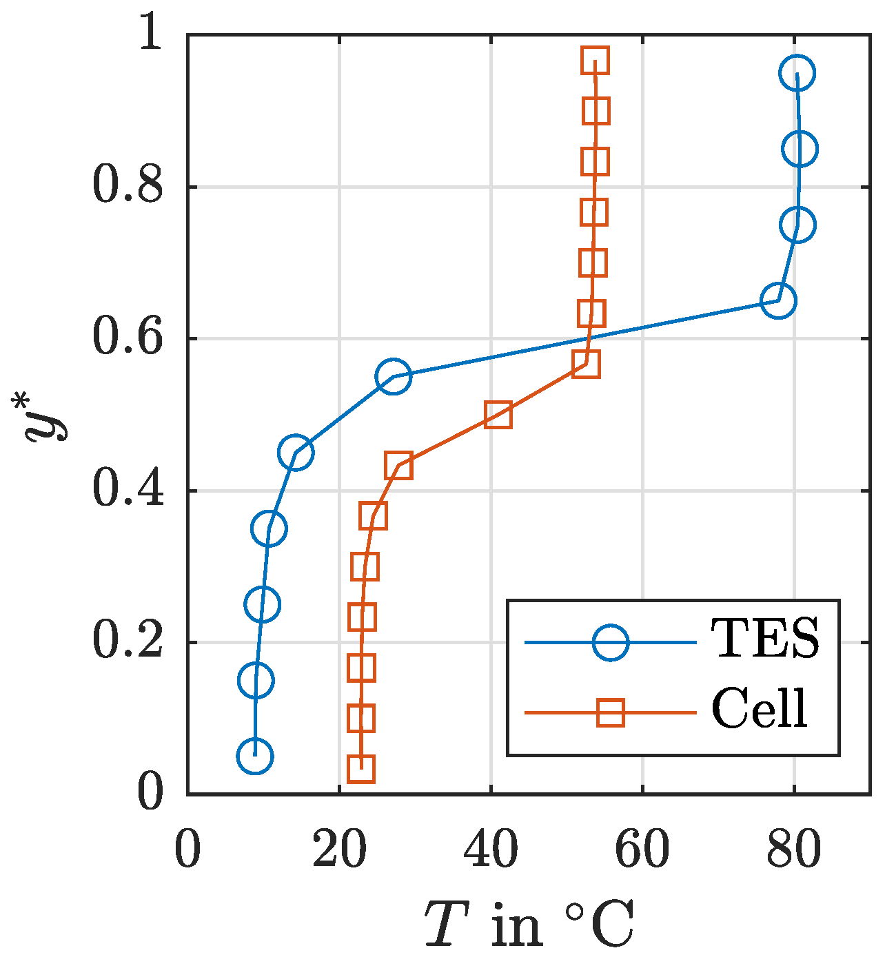
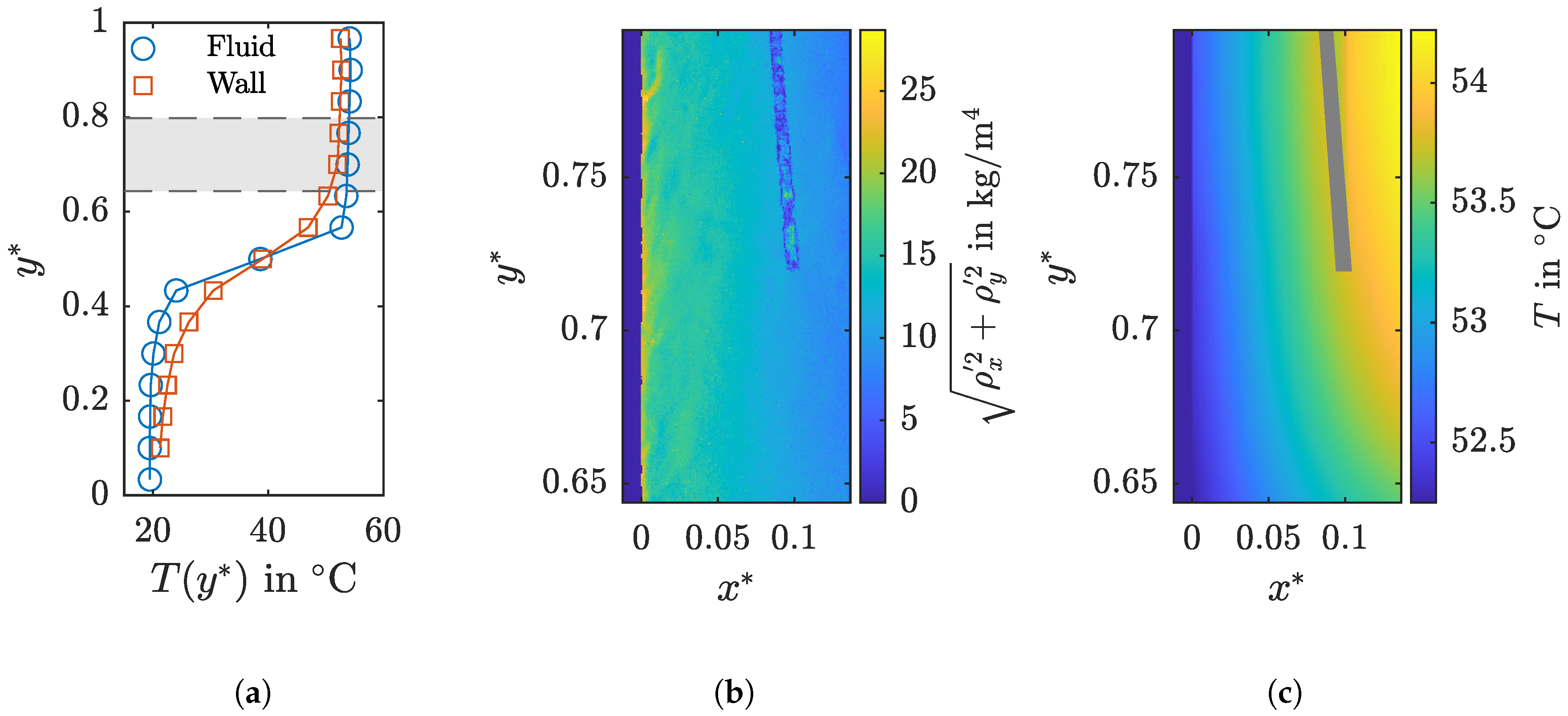
To test the measuring principle and the evaluation procedure of the BOS method described in the previous section, measurements in the region of the convective wall jet shown by the velocity measurements have been done. Therefore, the measuring cell has been filled with a stratification shown in
Figure 10a by vertical temperature profiles measured in the fluid and the aluminium wall, respectively. The dashed lines indicate the height the measurement has been taken and show that the entire field of view lies in the hot layer of the stratification, but also not far above the thermocline. Therefore, the temperature of the aluminium wall in the lower part of the field of view already decreases. The temperature of the water in this region is nearly the same as in the whole field of view. In comparison to the PIV measurements, the field of view has become larger as the distance between the camera and measuring cell has been adjusted to focus on the background picture.
Figure 10b,c show instantaneous snapshots of the magnitude of the density gradient and the resulting temperature field five minutes after filling the measuring cell. To calculate those, the raw images of the measurements have been evaluated by the PIV algorithm with a size of the interrogation window of
and an overlap of 50% which results in a spatial resolution of the camera in the mid-plane of the measuring cell of
and a region of
that is represented by one displacement vector. Before calculating the density gradients from the displacement vector field, a median filter has been applied that removes vectors which are more than two times bigger than the median of their neighbours in a region of
vectors and replaces them with the median vector [
31]. This step has been applied as all incorrectly evaluated values get summed during the integration of the density gradient.
To be able to calculate the absolute density, as discussed in the previous section, additional temperature sensors have been installed in the measuring cell. One sensor was positioned in a distance of
to the wall surface and can be seen on the upper right side of
Figure 10b. The bottom part of this sensor has been chosen to be the starting point of the integration of the density gradients as the density in this position can be found by the measured temperature. The area of the sensor is masked in grey in the temperature field of
Figure 10c to indicate this starting point, and since the evaluation of the temperature in this area is influenced by the sensor. Another temperature sensor has been glued on the wall surface at the height of
to work as a verification spot for the finally evaluated temperature field. Due to its small size, it cannot be seen in the evaluated images.
The magnitude of the density gradient field shows the highest density gradient on the left side attached to the surface of the aluminium wall (at ) with up to . With increasing distance to the wall surface, the density gradient decreases until it reaches its minimum value on the upper right part of the field of view with . A more precise look to the area with the high gradients shows that their decay from the left to the right side of the field of view is not steady as the gradients change between lower and higher values.
A high density gradient shows—even if it is not directly proportional—a region of a high temperature gradient. Therefore, the structures on the left side of the figure which are attached to the wall indicate local temperature differences. The temperature boundary layer of laminar, vertical convection would rise steadily from a lower temperature at the wall surface to a higher temperature in the bulk region of the measuring cell. Thus, the density gradient field of laminar vertical convection should be a steady decrease, which leads here to the result that the examined structures are a consequence of the turbulent velocity fluctuations that have been described in the discussion of the PIV measurements.
By looking at the temperature field in
Figure 10c these small structures cannot be seen as a local difference in temperature which shows that these differences are small compared to the temperature differences in the boundary layer. Nevertheless, the temperature boundary layer of the vertical convection is visible with low temperatures on the left side adjacent to the wall and high temperatures on the right side. These high temperatures increase in the upper right corner up to
, and they are thereby in a similar range as the temperature of the sensor in the middle of the cell. The thickness of the temperature boundary layer increases in the bottom part of the temperature field. The observation of the verticle temperature profiles in
Figure 10a shows that the temperature difference between water and wall in the lower part of the field of view gets higher. Thus, the heat flux from the water to the wall is higher in this region, which results in the thicker temperature boundary layer.
For verification, the BOS results are compared to the measured temperature of the sensor glued on the wall surface. At the time of the shown temperature field, the sensor has measured a temperature of . This value is equal (with respect to the uncertainty of ) to the temperature evaluated by the BOS measurement at this position. As a result, this shows that the BOS method is capable of measuring high-resolution temperature fields in transparent media.
Since not only one measurement image, but a short series of 200 images ( at sampling frequency) has been taken, the BOS method can be used to analyse the temporal development of the temperature. However, in this case, time-series data of the temperature at various locations in the field of view have not shown significant changes in temperature and are therefore not presented here. But in general, the long-term development of temperature can be studied with this method. It can also be used in experiments with higher temperature variations since the temporal limitation is the same is for single frame PIV measurements and is therefore only limited by the used camera.
Certainly, it is to mention that temperature measurements with the BOS method are subject to some restrictions which are to be considered before applying the technique. Gradients of the refractive index which occur parallel to the viewing direction of the camera (at small angles of the aperture of the camera this corresponds here to the z-axis in good approximation), do not lead to a distortion of the background and therefore cannot be measured. Besides, all gradients of the refractive index that occur in the x- or y-direction are summed over the entire depth of the measuring cell in the z-direction.
In the presented case, the influences of these restrictions are relatively small. Due to the stable thermal stratification of the water and the camera’s viewing direction parallel to the wall, strong density gradients do not occur in the viewing direction. Thus, the technique is capable of evaluating most of the occurring changes in refractive index, and therefore the resulting temperature distribution should be in good agreement to the real temperature field in the measurement plane.
In contrast, when interpreting the structures in the density gradient field, care must be taken to ensure that they are integrated over the entire depth of the cell. This leads to the problem that an observed structure cannot be matched to a particular position in the z-direction. One possibility to solve this issue would be to perform simultaneous PIV and BOS measurements and to correlate time-series data of the density gradients and the velocity. Structures in the density gradient field that do not correlate with the velocity would then have to be in another z-position.


