Force and Stress Simulation in Experimentable Digital Twins Using the Transfer Matrix Method

Abstract

Experimentable Digital Twins are capable of combining different simulation domains on a system level. This has been shown for a multitude of simulation domains, e.g., rigid body dynamics, control, sensors, kinematics, etc., and application scenarios, e.g., automotive, space, and industrial engineering. In our work, we investigate how to include structural loads into an Experimentable Digital Twin while maintaining computational efficiency and interoperability on a system level. We combine rigid body dynamics with the transfer matrix method to simulate forces and stresses. We show our approach for statically determinate beam structures in a simulation on a system level and validate it experimentally and numerically with static and dynamic example problems. The results show a strong agreement in these comparisons, confirming the accuracy and reliability of our method. For practical applications, we see force and stress simulation using the transfer matrix method as an additional tool to facilitate simulation-based engineering in the early stages of structural design processes, e.g., when dealing with uncertain loading conditions and operational complexity on a system level.

1. Introduction

1.1. Motivation

An Experimentable Digital Twin (EDT) combines different simulation domains and ensures the technical and semantic interoperability of the individual models and algorithms. Thus, it represents a sophisticated mapping of the behavior of its existing or future real twin (RT) [1]. An EDT can be used for a wide variety of simulation-supported methods and processes. When it comes to mechatronics and the design or optimization of systems and their components, the (future) forces, moments, and torques acting within the system determine a lot of the specifications of the real-world asset (material, shape, fabrication, etc.). Thus, simulation methods analyzing forces, moments, and torques are crucial in EDTs when it comes to a detailed system representation for mechatronics. Figure 1 showcases the authors’ vision of an EDT stress simulation of a real-world asset on a system level (cf. Section 2.1 for more detail).

When it comes to classical computational methods to analyze forces in systems, rigid body dynamics (RBD) and finite element analysis (FEA) are used. RBD is used to solve the equations of motion and calculate the dynamic behavior of multi-body systems. It is considered fast in terms of computational speed and, in many cases, even real-time capability. FEA is used for stress and deformation analysis in the context of structural mechanics. As this numerical method is solving complex systems of partial differential equations, it is rather time-consuming but delivers very detailed results. Combined approaches of RBD and FEA exist (cf. Section 1.2).

However, today’s combinations of RBD and structural simulations are limited when it comes to simulation capabilities at a system level, as required for simulation-supported methods for EDTs. Typical limitations include the barrier of an appropriate time-stepping algorithm and model exchange, technical and semantic interoperability, and complexity.

In the present work, we suggest a coupling of RBD and the transfer matrix method (TMM) to facilitate force and stress simulation in an EDT on a system level. Our approach aims to resolve the currently observed incompatibility of a rather broad but fast model on a system level and a very detailed view of single components that comes at high computational costs. The presented approach enables simulation-based section force and stresses investigation in EDTs for different application scenarios at a system level. This is shown in the example of beam structures within an existing framework for EDTs.

1.2. State of the Art

Enabling EDTs to produce reliable structural simulations is essential in various application areas, such as automotive engineering, aerospace, robotics, and medical technology. Nevertheless, there are only a few valid and practically applicable approaches since crucial simulation methods involved rely on a variety of different physical and mathematical models.

At present, the coupling of RBD with structural simulations is moving further into the center of current research as systems are being designed to meet ever more stringent requirements. Preliminary work in this field does not deal with all-encompassing simulations but with individual aspects of them, e.g., only the control, dynamics, kinematics, structural behavior, etc. Therefore, all existing solutions for the coupling of RBD and structural simulations are either very theoretical and, therefore, not yet practical in general applications or exclusively specialized for a specific application.

The theoretical approaches deal with different co-simulation strategies [2,3], especially for FEA, and develop sophisticated methods to extrapolate the behavior and time step management of individual systems [4,5]. Although these works make important contributions to basic research in the field of simulation-based interaction between RBD and FEA, they can hardly be used for practical applications due to the complexity of the underlying mathematical models and due to rather large simplifications. In addition, all approaches have major problems with a time scale close to real-time capability, which is becoming increasingly important in today’s development processes (e.g., in the context of interactive analysis or virtual commissioning). Nevertheless, some attempts are being made to achieve a fast and efficient FEA coupling. In a previous study [6], a control engineering problem is specifically considered, and initial experiments are already being carried out. In a previous study [7], robotic path planning in the presence of deformable objects is presented and extended to a mathematical model that ultimately analyzes the material properties with the help of a robot. First, frameworks try to couple RBD and FEA by creating interfaces between different independent programs [8] or by including rigid body motion in FEA [9]. However, the focus is on the investigation of individual components rather than the whole system. The Floating Frame of Reference Formulation approaches the problem completely from the RBD side but has major disadvantages in terms of performance, robustness, and workload [10] and is, therefore, not very common.

Another bracket of approaches solves the coupling problem from a phenomenological point of view, i.e., an integration of structural mechanical results is performed rather than a classical co-simulation. A common method is to record the maximum forces acting on a component of the system during a motion sequence, e.g., a durability test is carried out with a structural simulation [11,12]. Another widespread application of structural mechanics results is to investigate undesirable vibrations in technical systems. A modal analysis helps to investigate effects that cannot be seen in a simulation based purely on RBD [13]. The automotive and aerospace industries, in particular, are showing enormous interest in incorporating structural mechanics results into the overall system simulation [14].

A coupling of general Digital Twins (DT) with FEA is presented in [15]. Although this is demonstrated with an experiment, there is no description of the coupling mechanisms and algorithms used and no evaluation of the results, so no statements can be made here about the validity, structure, or applicability of the approach or the usage of RBD. A successful coupling of a real-world asset and an FEA-DT is presented in [16]. However, the focus is purely on structural simulations, and no statements on the interaction with other physical simulations are made.

Overall, there is a lack of efficient ways to combine RBD and structural mechanics that are not only application-independent but also consider, at the same time, other important simulation domains, as it is performed in an EDT.

1.3. Preliminary Works of the Authors

In preliminary works focusing on the coupling of RBD and structural simulation, relevant variables (forces and moments, information on degrees of freedom) of the RBD were extracted and used as input variables for a structural simulation, as well as the knowledge gained from the FEA (displacements) was given back into an RBD. A new type of joint was introduced, which is physically based on a “non-linear compression spring” with a variable spring constant [17]. However, this is a phenomenological description of the effect of structural-mechanical deformations within complex mechatronic systems, which uses previously calculated FEA results and does not run in parallel with the actual structural simulation, so spontaneous changes are no longer possible. A direct coupling between RBD and finite element method (FEM) was developed by using commercial software (Ansys mechanical [9]) for structural calculations [18]. The relevant variables are exchanged via files, and several user modes are possible, including a parallel calculation in which the user requests a structural simulation from the RBD framework [19]. With this method, several relevant research questions could be solved, for example, on the use of materials in space robotics/satellite technology [20] or on the influence of the quality of control algorithms on structural deformations [21]. However, the major disadvantage of this coupling method is the lack of obtaining results fast, as this property is not inherent in the FEA used. The RBD pauses during an FEA calculation, which can take any length of time depending on the complexity of the model.

The idea for this work is based on a simulation of elastic components within the RBD using an analytical structural calculation algorithm directly integrated there, which can also run in real time, as has already been shown in a first proof of concept [22]. In a conference paper [23], the authors pointed out potential benefits of including structural calculations into EDTs for structural applications, e.g., the detection of unpredicted and undesirable fatigue behavior of systems in virtual prototypes.

2. Methods and Concept

In our approach, RBD and TMM are coupled in an EDT framework. The RBD solves the equation of motion. Kinematic data and constraint forces are passed to the TMM for structural calculations.

2.1. Experimentable Digital Twin

The use of the term “Digital Twin” in relation to technical systems goes back to Michael Grieves (2003) [24]. In 2010, NASA took up the concept for aerospace and used it to describe an “ultra-realistic simulation” [25]. The term was subsequently examined in many disciplines, e.g., from the perspective of simulations, cyber-physical systems, or production technology [26]. In 2018, Gartner classified DT as part of the digitalized ecosystem as one of the five key technological trends and predicted that the technology would reach the “productivity plateau” in 5–10 years [27]. Nowadays, examples of real-world engineering applications of DT exist, e.g., DT to adapt and optimize the layout of reconfigurable manufacturing cells [28], DT for safety critical robotics [29], and DT for monitoring and predictive maintenance of airframes and pipelines [30,31]. Simulation, as one of the basic technologies for DT, is a recognized standard in many industries, such as mechanical engineering. Simulation methods and algorithms are used throughout the entire development process. Even if each simulation method solely provides valuable insights, there is still a lack of a cross-system and cross-disciplinary approach that also takes into account the interaction of components, environment, and disciplines and, thus, enables the consistent use of simulations in a uniform methodology over the entire life cycle. To this end, the DT is intended to combine all these simulation domains and the cross-life cycle use of simulation in a comprehensive concept. A corresponding framework [32,33] was developed at the MMI for this purpose, which brings DT to life and makes it executable, experimentable, and integrable [1]. Thus, in this work, we are using the term of an EDT, corresponding to [34].

As mentioned in Section 1.1, technical and semantic interoperability is a challenge when coupling a structural mechanics simulation to any other physical simulation [4]. This is mainly due to the mismatch in models and algorithms that make time stepping and model exchange particularly difficult. We dealt with this general problem of co-simulation by running the TMM in each time step of the RBD simulation as a direct plugin within the EDT framework. Using this design, the TMM depends on the validity of the RBD simulation, and, as a consequence of this coupling, means that all limitations of the RBD simulation are inherited by the TMM (cf. Section 5).

2.2. Rigid Body Dynamics

RBD is a numerical simulation method in which complex systems are divided into individual rigid bodies that are connected to each other by joints and consequently constrained in certain directions of movement. Thus, by setting up and solving the equations of motion, trajectories of the resulting velocities, accelerations, and positions of the individual bodies, and the resulting forces and torques can be generated.

In the context of mechatronic systems, inverse dynamics are usually performed, as the forces resulting from a movement have to be calculated. Today, RBD is a standard component of various physics simulators [35,36]. In general, a rough distinction is made between Newton–Euler and Lagrangian methods [37]. In the present project, a Newton–Euler method with a maximum coordinate approach is principally applied [38] since the constraining forces acting between rigid bodies are required for the transfer matrix method, which Lagrangian methods do not provide explicitly. There are various methods for solving the problem numerically. The impulse-based approach [39] is established as it is very stable (due to the elimination of a further integration process between force and position) and leads to a linear complementarity problem, which can always be solved using, e.g., Lemke’s algorithm. The impulse-based approach has also been extensively investigated and used for various applications by several of the authors [38].

2.3. Transfer Matrix Method

In structural mechanics, the transfer matrix method (TMM) is used as a computational method during preliminary design [40,41]. Many structures consist of recurring structural elements (beams, plates, shells, etc.) whose behavior can be described by differential equations. Transfer matrices represent an analytical solution of these differential equations. A state vector ${\overrightarrow{\mathrm{u}}}_0$, describing the elastic state at position 0, is mapped on the state vector ${\overrightarrow{\mathrm{u}}}_1$, describing the elastic state at position 1 with distance $\mathrm{l}$ to position 0, by the transfer matrix ${\overrightarrow{\overrightarrow{\mathrm{W}}}}_0$:

$${\overrightarrow{\mathrm{u}}}_1={\overrightarrow{\overrightarrow{\mathrm{W}}}}_0{\overrightarrow{\mathrm{u}}}_0$$

(1)

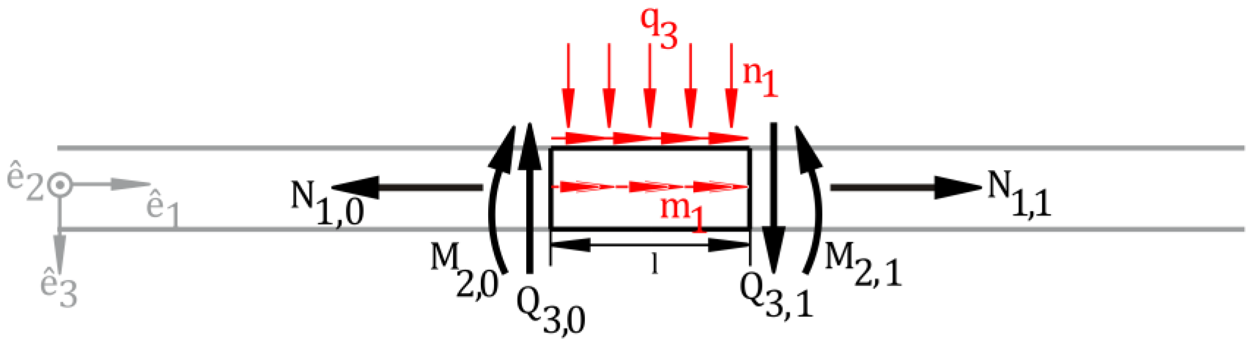
For beams under bending about the ${\mathbf{e}}_2$-axis, the differential equations describing the relationship between line load ${\mathrm{q}}_3$, section force ${\mathrm{Q}}_3$ and section bending moment ${\mathrm{M}}_2$ (according to Figure 2) are as follows:

$${\displaystyle \frac{\mathrm{d}{\mathrm{Q}}_3}{\mathrm{d}{\mathrm{x}}_1}}=-{\mathrm{q}}_3;{\displaystyle \frac{\mathrm{d}{\mathrm{M}}_2}{\mathrm{d}{\mathrm{x}}_1}}={\mathrm{Q}}_3.$$

(2)

The relationships between the section forces and moments on the left side of a beam interval and on its right side are described explicitly by solving the following differential equations:

$${\mathrm{Q}}_{\mathrm{3,1}}=-{\mathrm{q}}_3 \mathrm{l}+{\mathrm{Q}}_{\mathrm{3,0}}$$

(3)

$${\mathrm{M}}_{\mathrm{2,1}}=-{\displaystyle \frac{1}{2}}{\mathrm{q}}_3{\mathrm{l}}^2+{\mathrm{Q}}_{\mathrm{3,0}}\mathrm{l}+{\mathrm{M}}_{\mathrm{2,0}}$$

(4)

These equations can be displayed in a compact manner using a transfer matrix:

$$\left(\begin{array}{c}{\mathrm{M}}_{\mathrm{2,1}}\\ {\mathrm{Q}}_{\mathrm{3,1}}\\ 1\end{array}\right)=\left(\begin{array}{ccc}1& \mathrm{l}& -{\displaystyle \frac{{\mathrm{q}}_3{\mathrm{l}}^2}{2}}\\ 0& 1& -{\mathrm{q}}_3\mathrm{l}\\ 0& 0& 1\end{array}\right)·\left(\begin{array}{c}{\mathrm{M}}_{\mathrm{2,0}}\\ {\mathrm{Q}}_{\mathrm{3,0}}\\ 1\end{array}\right)$$

(5)

With the same procedure, the transfer matrix for a three-dimensional beam element is derived, including skewed bending, torque, and forces in the direction of the longitudinal beam axis:

$$\left(\begin{array}{ccccccc}1& 0& 0& 0& 0& 0& -{\mathrm{m}}_1\mathrm{l}\\ 0& 1& 0& 0& 0& \mathrm{l}& -{\displaystyle \frac{{\mathrm{q}}_3{\mathrm{l}}^2}{2}}\\ 0& 0& 1& 0& -\mathrm{l}& 0& {\displaystyle \frac{{\mathrm{q}}_2{\mathrm{l}}^2}{2}}\\ 0& 0& 0& 1& 0& 0& -{\mathrm{n}}_1\mathrm{l}\\ 0& 0& 0& 0& 1& 0& -{\mathrm{q}}_2\mathrm{l}\\ 0& 0& 0& 0& 0& 1& -{\mathrm{q}}_3\mathrm{l}\\ 0& 0& 0& 0& 0& 0& 1\end{array}\right)$$

(6)

3. Implementation

This section explains how the TMM is implemented within the EDT framework and provides validation examples. Analytical solutions for these examples exist, and we compare the solution of our TMM implementation with these.

3.1. Coupling of RBD and TMM

The TMM makes available section forces and stresses in the EDT at a system level. In our approach, the TMM uses information from the EDT framework, mainly coming from the RBD. To calculate the section forces in a beam, the TMM uses information on the following:

• On the beam’s geometry and inertia;
• On the beam orientation with respect to the global coordinate system;
• On concentrated forces acting upon the beam, e.g., support forces;
• On volume forces acting upon the beam;
• On the beam’s velocity.

While the TMM uses information from the RBD, the RBD works independently from the TMM. While the coupling between these two domains is unidirectional, there can be an indirect feedback loop within the DT, e.g., if a control algorithm makes use of stress information and adjusts the velocity. Furthermore, the calculated quantities of a structural analysis (stress, bending moment, etc.) can be visualized in the EDT, which allows for a very fast and intuitive way of evaluating results and—globally speaking—structural decisions.

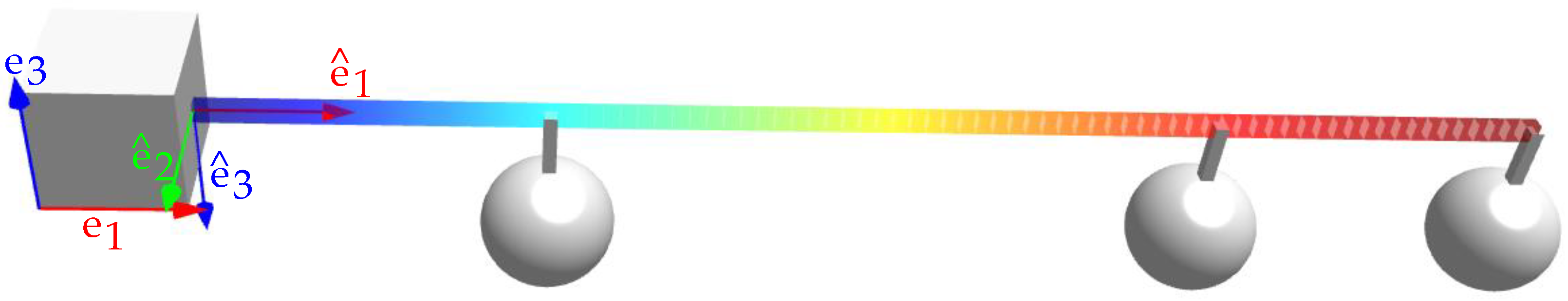
The beam orientation is retrieved as a transformation matrix $\mathbf{R}$ containing the direction cosines of the local beam coordinate system. With the matrix $\mathbf{R}$, force values given in the global coordinate system are mapped into the local beam coordinate system. All section forces and stresses are calculated in the local beam coordinate system starting at the beam end, with ${\widehat{\mathbf{e}}}_1$ being the direction of the beam’s longitudinal axis (see Figure 3).

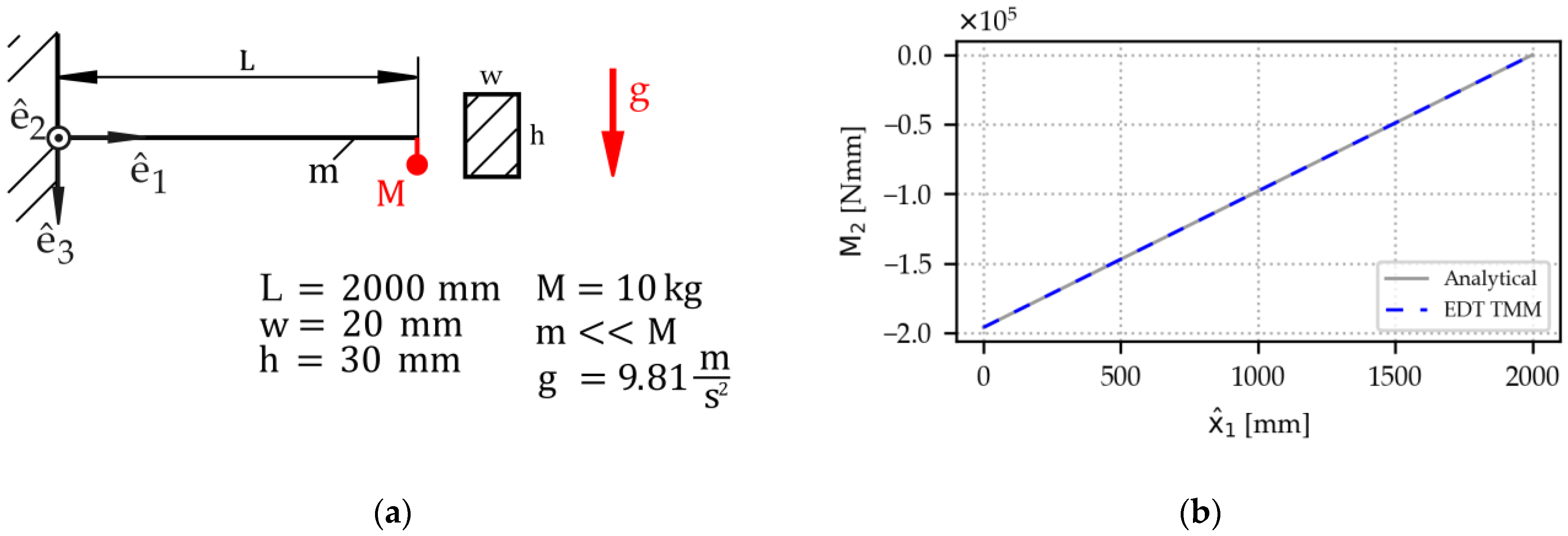
Example 1. 

A cantilever beam is subject to a tip load (Figure 4). The load is implemented as a single mass under gravity; the beam weight is chosen to be negligibly small. The TMM uses the support force provided by the RBD on the beam’s left end and calculates the remaining section forces by multiplying matrix (6) for each interval. Line loads are all zero for this example. Matching the analytical solution, the TMM’s bending moment output shows a linear course of the curve from support to tip.

3.1.1. Handling of Concentrated Forces and Moments

The TMM handles concentrated forces and moments that are introduced at any given point of the beam by multiplying a transfer matrix for an interval of zero length. Examples of such concentrated forces are joint forces introduced by additional joints or contact forces. For example, the matrix for a transversal load $\mathrm{P}$ in ${\widehat{\mathbf{e}}}_2$-direction would be as follows:

$$\left(\begin{array}{ccccccc}1& 0& 0& 0& 0& 0& 0\\ 0& 1& 0& 0& 0& 0& 0\\ 0& 0& 1& 0& 0& 0& 0\\ 0& 0& 0& 1& 0& 0& 0\\ 0& 0& 0& 0& 1& 0& -\mathrm{P}\\ 0& 0& 0& 0& 0& 1& 0\\ 0& 0& 0& 0& 0& 0& 1\end{array}\right)$$

(7)

In our implementation of the TMM, the matrix is multiplied either before (i.e., left end) or after (i.e., right end) the interval in which the concentrated force acts on the beam. This leaves a discretization error, which remains negligible if the interval length is set to be short. The capacity to handle concentrated forces along acting arbitrary points along the beam axis is demonstrated by Example 2.

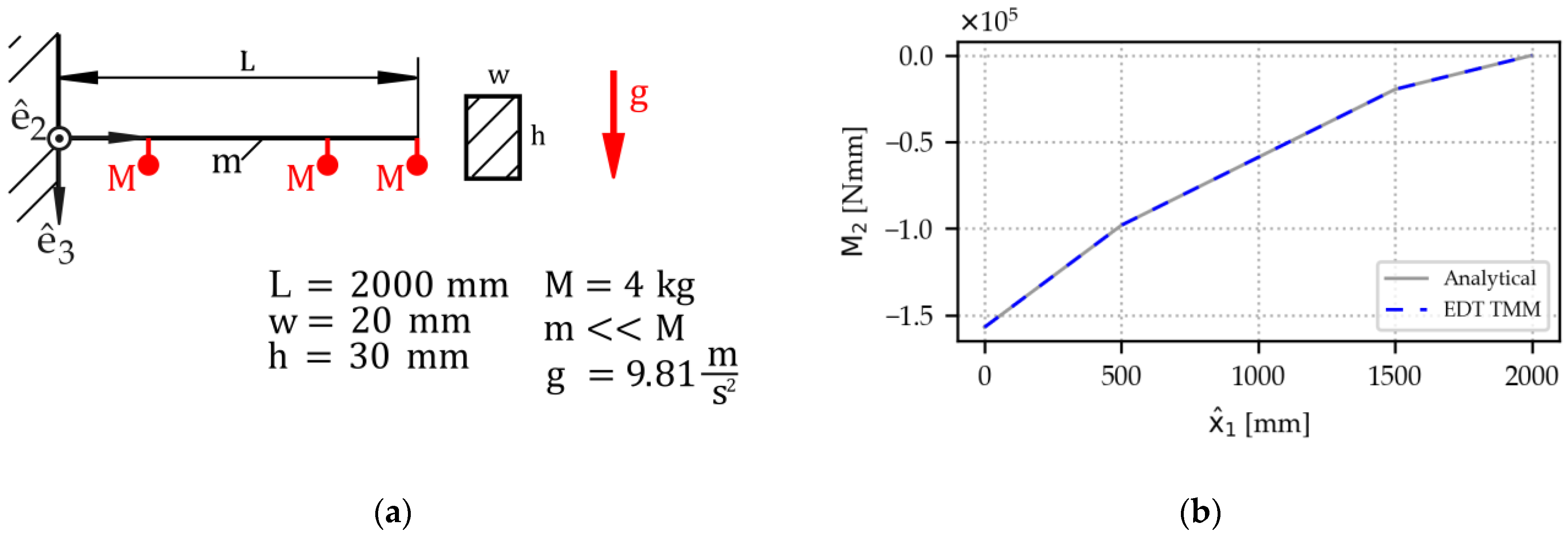
Example 2. 

A cantilever beam is subjected to three loads along its beam axis (Figure 5). Loads are implemented as a single mass under gravity; the beam weight is chosen to be negligibly small. Matching the analytical solution, the TMM’s bending moment output shows a piecewise linear course, with discontinuities in the derivative at the points of load introduction.

3.1.2. Handling of Gravitational Forces

RBD and TMM handle volume forces differently. In RBD, volume forces are typically treated simply as concentrated forces in the center of mass (COM). For the TMM, this simplification would result in a discontinuity like described above in Section 3.1.1., and this would not accurately reflect section forces along a beam’s axis. In our implementation of the TMM, the information on gravitational forces is picked up as a concentrated force from the RBD, then mapped onto the local beam coordinate system, and then transformed into a line load by dividing it by the total beam length. These line loads are included in the last column of every interval’s transfer matrix, according to matrix (6). The capacity to handle gravitational loads is demonstrated in Example 3.

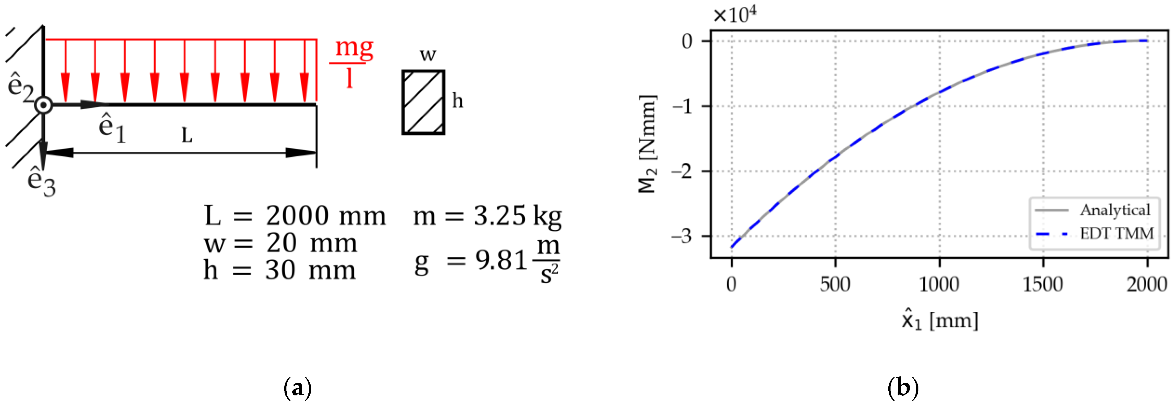
Example 3. 

A cantilever beam under gravity (Figure 6). The beam’s mass corresponds to an aluminum beam. Matching the analytical solution, the TMM’s bending moment output shows a quadratic function.

3.1.3. Handling of Dynamic Scenarios

In our implementation, the TMM computes the section forces in every time step of the dynamic simulation. Thus, it is also able to compute section forces over time in a dynamic scenario. This is demonstrated in Example 4, for which an analytical solution exists.

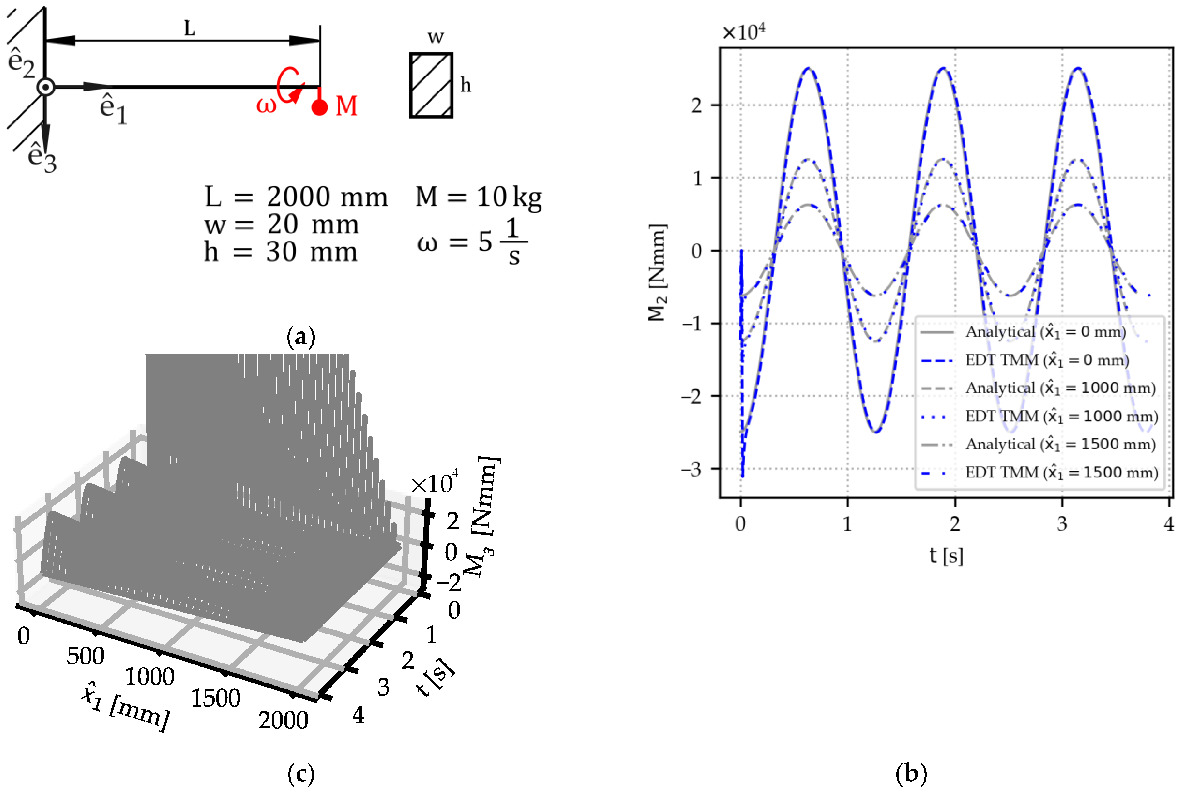
Example 4. 

A cantilever beam with a rotating point mass at its tip (Figure 7). Gravity is not considered to facilitate understanding. The bending moment about the ${\widehat{\mathbf{e}}}_2$-axis over time is plotted for three different locations along the beam axis (Figure 7b). The TMM’s bending output matches the analytical solution, except for initial time steps in which a motor with unlimited torque accelerates the point mass up to the specified angular velocity. Figure 7c shows a surface plot of the bending moment about the ${\widehat{\mathbf{e}}}_3$-axis over time to demonstrate the capabilities to handle skewed bending.

3.1.4. Handling of Inertia Forces

Inertia forces must be considered in scenarios where the beam subject to analysis is itself under movement. Inertia forces act in opposing directions to accelerations. In our implementation, the absolute acceleration in local beam coordinates is calculated at every midpoint of a beam interval, multiplied by the linear density, and applied as a constant line load in the matrix (6). Beam accelerations cannot be retrieved from the RBD, as the RBD works with an impulse-based approach. Information about beam movement is given as velocity and angular velocity at the beams center of gravity (COG) in the global coordinate system:

$${\dot{\mathbf{x}}}_{\mathbf{S}\mathbf{P}}={\mathrm{x}}_{\mathrm{i}}{\mathbf{e}}_{\mathbf{i}};\hspace{1em}\dot{\mathsf{\omega }}={\mathsf{\omega }}_{\mathrm{i}}{\mathbf{e}}_{\mathbf{i}}$$

(8)

Accelerations are calculated using the difference between velocities over a time step:

$${\ddot{\mathbf{x}}}_{\mathbf{S}\mathbf{P}}={\displaystyle \frac{\mathsf{\Delta }{\dot{\mathbf{x}}}_{\mathbf{S}\mathbf{P}}}{\mathsf{\Delta }\mathrm{t}}};\hspace{1em}\dot{\mathsf{\omega }}={\displaystyle \frac{\mathsf{\Delta }\mathsf{\omega }}{\mathsf{\Delta }\mathrm{t}}}$$

(9)

Velocities and accelerations are transformed into the local beam coordinate system:

$$\dot{\mathbf{x}}={\widehat{\dot{\mathrm{x}}}}_{\mathrm{i},\mathrm{P}}{\widehat{\mathbf{e}}}_{\mathbf{i}};\hspace{1em}{\ddot{\mathbf{x}}}_{\mathbf{P}}={\widehat{\ddot{\mathrm{x}}}}_{\mathrm{i},\mathrm{P}}{\widehat{\mathbf{e}}}_{\mathbf{i}};\hspace{1em}\dot{\mathsf{\omega }}={\widehat{\dot{\mathsf{\omega }}}}_{\mathrm{i}}{\widehat{\mathbf{e}}}_{\mathbf{i}}$$

(10)

To calculate the acceleration at an arbitrary beam interval’s midpoint P, we exploit that the vector pointing from COG to P has only one component that runs along the beam axis:

$${\mathbf{x}}_{\mathbf{C}\mathbf{O}\mathbf{G},\mathbf{P}}={\widehat{\mathrm{x}}}_{1,\mathrm{C}\mathrm{O}\mathrm{G},\mathrm{P}}{\widehat{\mathbf{e}}}_1=\left(-{\displaystyle \frac{\mathrm{L}}{2}}+{\widehat{\mathrm{x}}}_{1,\mathrm{P}}\right){\widehat{\mathbf{e}}}_1,$$

(11)

where ${\widehat{\mathrm{x}}}_{1,\mathrm{P}}$ is the position of P along the beam axis. With the well-known laws of kinematics, accelerations are calculated for every midpoint of beam intervals. Accelerations times the linear density are applied as line loads in transfer matrices of moving beams to account for inertia forces. The formula for the line loads is as follows:

$${\mathrm{n}}_1{\widehat{\mathbf{e}}}_1+{\mathrm{q}}_2{\widehat{\mathbf{e}}}_2+{\mathrm{q}}_3{\widehat{\mathbf{e}}}_3=-{\displaystyle \frac{\mathrm{m}}{\mathrm{L}}}·{\ddot{\mathbf{x}}}_{\mathbf{P}}=-{\displaystyle \frac{\mathrm{m}}{\mathrm{L}}}·\left(\begin{array}{c} \left[{\widehat{\ddot{\mathrm{x}}}}_{1,\mathrm{P}}-\left({{\widehat{\mathsf{\omega }}}^2}_2+{{\widehat{\mathsf{\omega }}}^2}_3\right)\left(-{\displaystyle \frac{\mathrm{L}}{2}}+{\widehat{\mathrm{x}}}_{1,\mathrm{P}}\right)\right]{\widehat{\mathbf{e}}}_1 \\ +\left[{\widehat{\ddot{\mathrm{x}}}}_{2,\mathrm{P}}+\left({\widehat{\dot{\mathsf{\omega }}}}_3+{\widehat{\mathsf{\omega }}}_1{\widehat{\mathsf{\omega }}}_2\right)\left(-{\displaystyle \frac{\mathrm{L}}{2}}+{\widehat{\mathrm{x}}}_{1,\mathrm{P}}\right)\right]{\widehat{\mathbf{e}}}_2 \\ +\left[{\widehat{\ddot{\mathrm{x}}}}_{3,\mathrm{P}}+\left(-{\widehat{\dot{\mathsf{\omega }}}}_2+{\widehat{\mathsf{\omega }}}_1{\widehat{\mathsf{\omega }}}_3\right)\left(-{\displaystyle \frac{\mathrm{L}}{2}}+{\widehat{\mathrm{x}}}_{1,\mathrm{P}}\right)\right]{\widehat{\mathbf{e}}}_3\end{array}\right)$$

(12)

The components of a line load are then included in the last column of the transfer matrix X.Y for a beam interval. The capacity to handle inertia loads is demonstrated in Example 5.

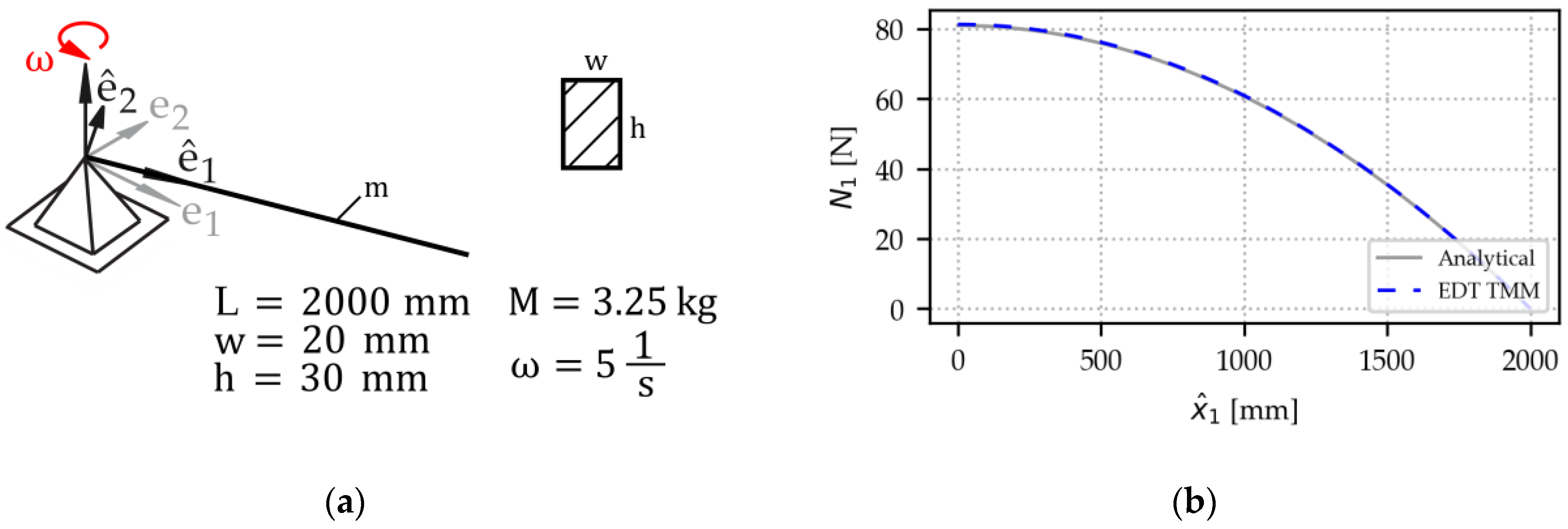
Example 5. 

A beam rotating with constant angular velocity (Figure 8). The beam’s mass corresponds to an aluminum beam. Gravity is not considered in this example. Matching the analytical solution, the TMM’s longitudinal force output shows a quadratic function.

3.1.5. Handling of Scenarios with Combined Phenomena

The EDT TMM implementation is able to handle combinations of the above-described scenarios. Example 6 shows this capacity along with a limitation.

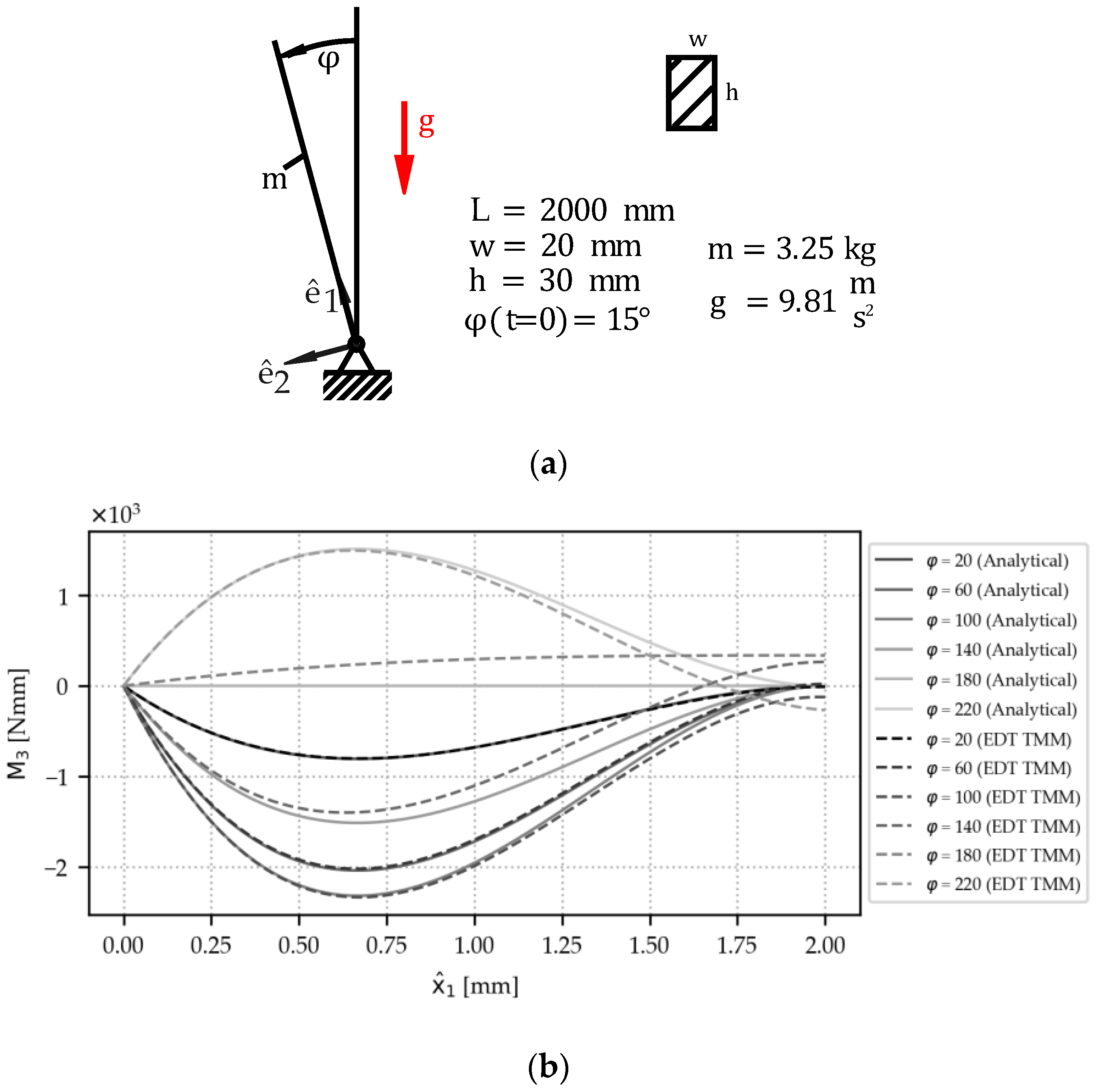
Example 6. 

A pin-ended beam under gravity (Figure 9a). The beam’s mass corresponds to an aluminum beam. The initial velocity of the beam is zero. While the nonlinear differential equation governing this movement cannot be resolved in the time domain, an analytical solution for the bending moment as a function of $\phi$ can be derived:

$$M_3\left({\widehat{x}}_1\right)=-{\displaystyle \frac{{\widehat{x}}_1}{L}} · {\displaystyle \frac{{\left(L-{\widehat{x}}_1\right)}^2}{L}} · {\displaystyle \frac{mg}{4}}\mathit{sin}\phi$$

(13)

The TMM does not fully match the analytical solution at the free end of the beam in this highly dynamic scenario. Nonetheless, the deviation from the analytical solution is negligible at the position of the maximum bending moment ${\widehat{\mathrm{x}}}_1={\displaystyle \frac{\mathrm{L}}{3}}$ (Figure 9b). The reasons and implications of the mismatch at the free end of the beam are discussed in Section 5.

4. Example Use Case

We apply our coupling of RBD and TMM within an EDT framework to a lab-scale demonstrator use case (see Figure 10). The use case is designed to contain features of a real-life application, such as a crane boom of a construction or forestry vehicle; a similar design was first proposed by the authors in [23]. The lab-scale demonstrator includes an actuator and three beam elements. Static and dynamic experiments are carried out to validate the TMM. Static scenarios are also used to compare the accuracy of the TMM to well-established analytical and numerical calculation methods. Dynamic scenarios are used to highlight the benefits of the system-level EDT. This section gives a detailed description of validation models, as well as experimental results.

4.1. Methods

4.1.1. Experiment

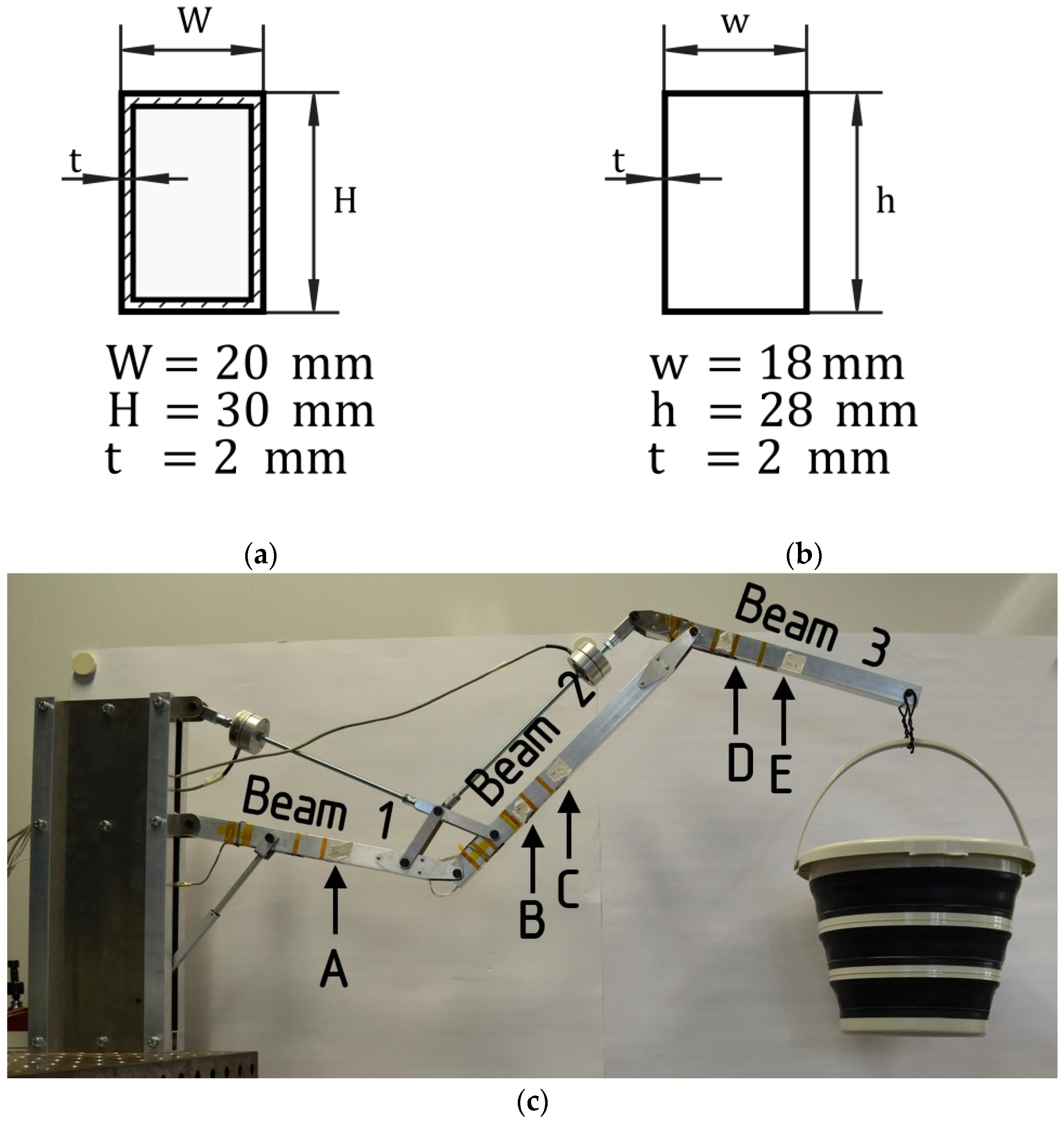
The lab-scale demonstrator forms a mechanism with one degree of freedom, able to move a load in a vertical plane. The mechanism consists of three beams, two rods, some linking elements, and a linear actuator. They are connected by hinge joints. The aluminum beams have lengths of 395 to 450 mm and a box cross-section with an edge length of 20 times 30 mm and a thickness of 2 mm (see Figure 11). The horizontal range, measured from frame to load introduction point, is between 610 and 1020 mm. The mechanism is powered by a 12 V linear actuator with potentiometer feedback, 200 N maximum load, and 100 mm stroke length, which is limited to a range between 28 and 100 mm by the mechanism.

The lab-scale demonstrator has one position for load introduction and five positions for load sensing. Load introduction is achieved using a bucket (0.51 kg) and standard mineral water bottles of 500 mL, each of them representing a load of 5 N. Load sensing is achieved through strain gauges. At each strain sensing position (A to E), two strain gauges at either side of a beam are wired in a half-bridge configuration that is sensitive to bending strain and insensitive to axial strain.

Experiments for the use case provide both static and dynamic strain values at discrete locations of the beams. However, it provides only information on bending moments, not on axial forces. To check for repeatability, we carried out each experimental scenario three times.

4.1.2. Digital Twin Model

The EDT must reflect all aspects of the real counterpart that are relevant to the respective application. In this case, the focus is on the structural-mechanical construction of the lab-scale demonstrator. Figure 12 shows the mechanical design with the specific component and axis names and, thus, the basic system structure. In contrast to a purely functional simulation model, the EDT reproduces this real physical system structure one-to-one in its model structure.

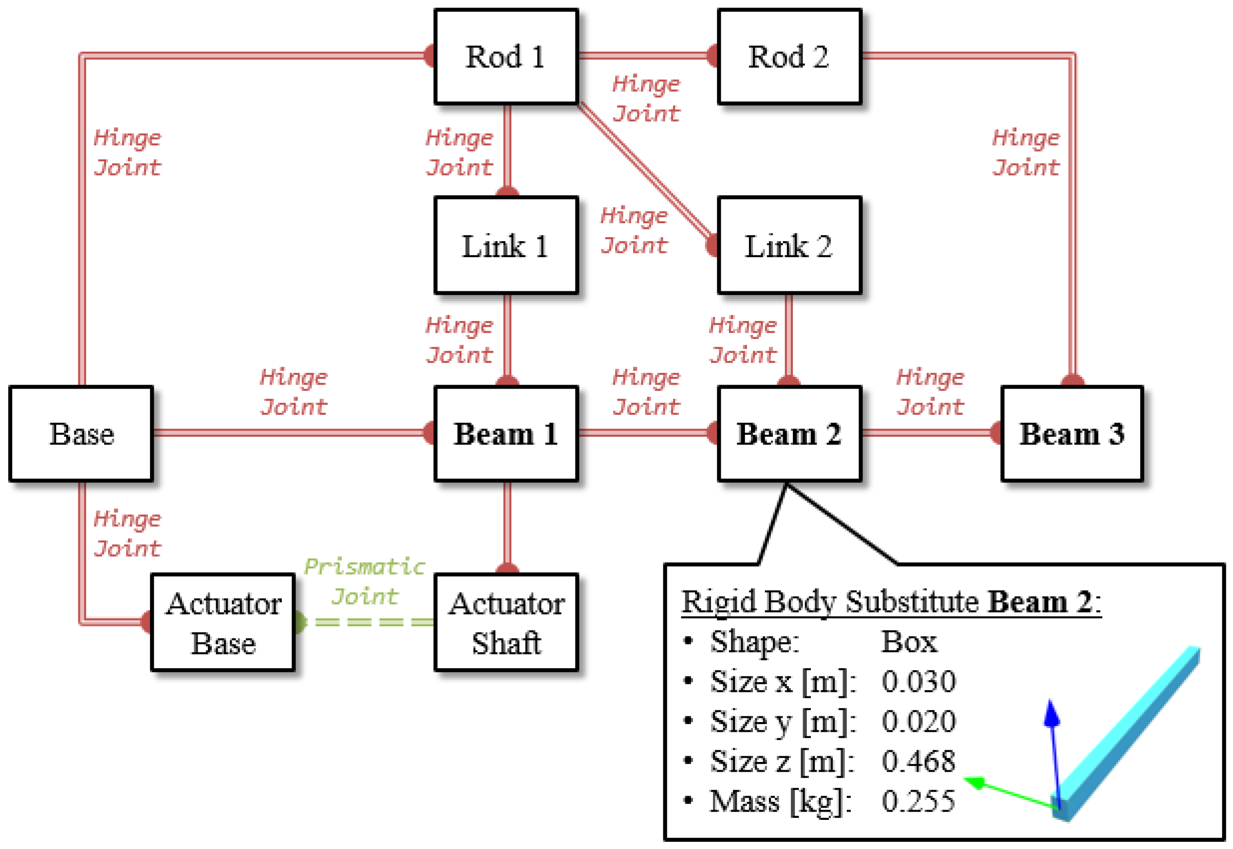
For each individual component, the EDT contains elementary model elements that are suitably linked within and between the respective simulation domains and thus assembled into an executable model. Figure 13 shows the resulting model topology in the rigid body dynamics domain. Here, the mechanical connections (joints) of the components are modeled as rigid bodies, and thus, the available degrees of freedom are defined.

Hinge joints offer exactly one rotational degree of freedom, while the actuated prismatic joint offers exactly one translational degree of freedom. The lab-scale demonstrator forms several closed kinematic chains, which significantly increases the system’s complexity. The kinematic movement of the arm, which is limited to one degree of freedom in the x–z plane, can be analyzed in the virtual model. 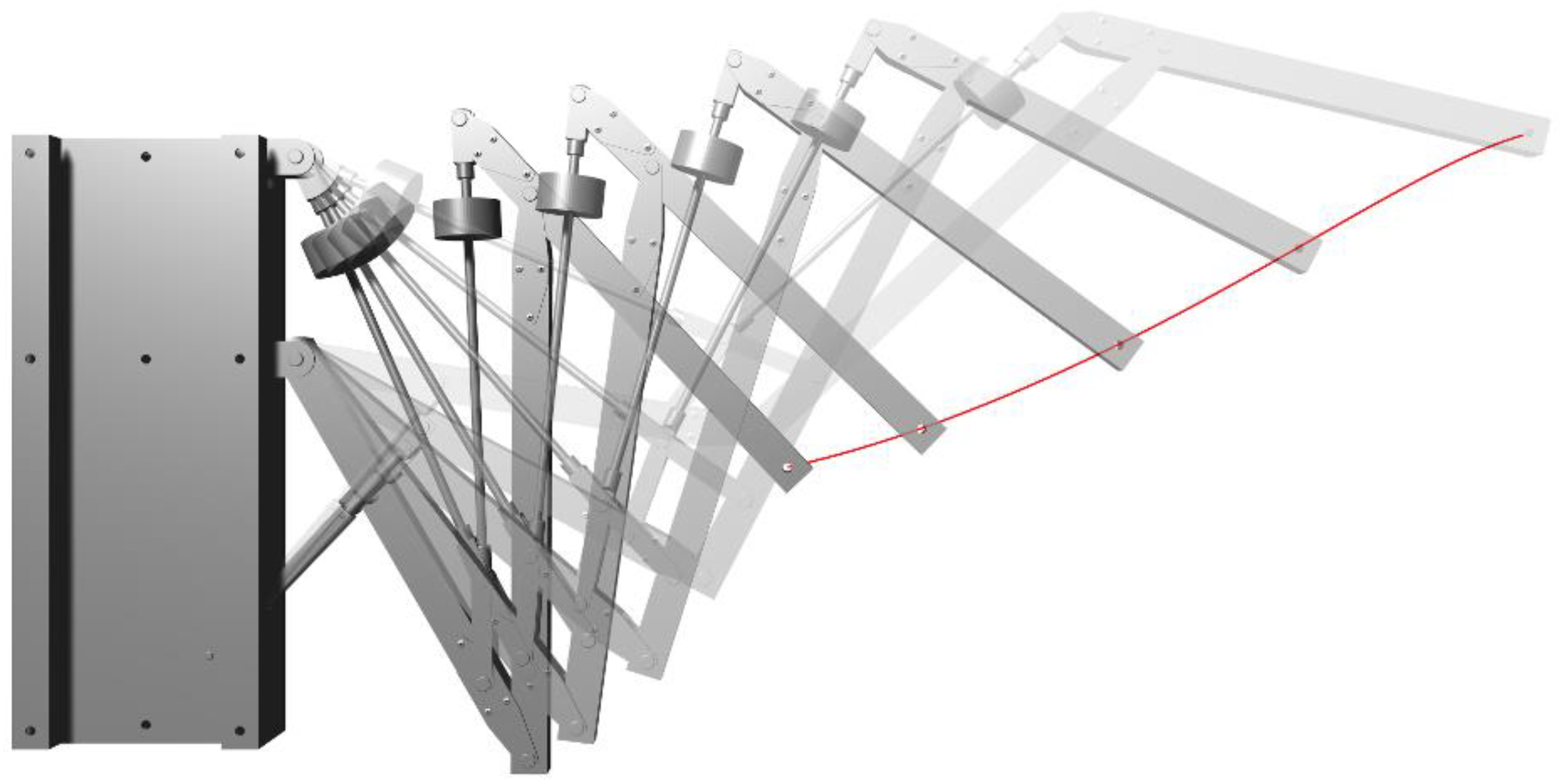Figure 14 shows the resulting trajectory of the arm tip at A11 (tool center point, TCP) and, thus, the kinematic workspace of the lab-scale demonstrator.

The dynamic simulation also takes into account the acting forces and moments. These form the basis for the coupling with the structural-mechanical simulation within the EDT. During simulation runtime, constraining forces in the joints calculated by the RBD are continuously passed on to the TMM, which can calculate and visualize various structural and mechanical variables such as shear, normal, and equivalent stresses using the TMM.

The TMM is implemented using the same EDT framework plugin described in Chapter 3. The beams are simplified as being non-stop from joint to joint, ignoring the metal fitting towards the joint. All beams are partitioned in 100 equidistant beam intervals. For stress calculations, the cross-sections are simplified as thin-walled box profiles (see Figure 11b), with shear and normal stresses calculated at 8 points in each cross-section (corners and midpoints).

For load introduction in the EDT, a pendulum bob with a fixed-set mass is applied on the tip of Beam 3.

The EDT for the use case provides static and dynamic values of section forces and stresses. Values for all locations on all three beams are available.

4.1.3. Numerical Model

The numerical model, based on the method of finite elements (FEM), used the Abaqus simulation framework [42] and employed second-order shell elements. The hinges were modeled by kinematically constraining the nodes in each geometric hole onto a reference point and coupling these reference points along an axis using hinge connector elements. Both a linear and non-linear analysis were performed, yielding near identical results due to the small loads and the absence of significant nonlinearity effects.

The numerical model for the use case provides static values of strains and stresses. Values for all locations on all beams are available.

4.1.4. Analytical Model

Analytical calculations are carried out, modeling the lab-scale demonstrator as a 2D Bernoulli beam structure. Section forces and moments were derived for this statically determinate system via equilibrium of forces and moments. For stress calculations, the cross sections are simplified as thin-walled box profiles (see Figure 11b); only normal stresses and strains are calculated for validation purposes.

The analytical model for the use case provides static values of section forces, strains, and stresses. Values for all locations on all three beams are available.

4.2. Scenarios

4.2.1. Static Scenario

Static scenarios are tested at three different actuator positions (28, 64, and 100 mm). For the experiments, all strain values are set to zero with an empty bucket (0.51 kg or 5 N), then six standard mineral water bottles of 500 mL are added, summing up to 3.06 kg in additional weight, which represents 30 N in additional force. For the EDT, a pendulum bob with a mass of 3.57 kg is applied on the tip of Beam 3, representing 35 N. When comparing EDT results to experiments, the results of a baseline scenario with a pendulum bob of 0.51 kg are subtracted to account for zero-setting with an empty bucket. For the numerical and analytical models, a vertical concentrated force of 30 N is applied.

4.2.2. Dynamic Scenario

Dynamic scenarios are tested from maximum to minimum stroke (100–28 mm), as well as maximum to middle to minimum stroke (100–64–28 mm). For the experiments, all strain values are set to zero with an empty bucket at the initial position, then six standard mineral water bottles of 500 mL are added, adding up to a total of 3.57 kg, including the bucket. For the EDT, a bob of 3.57 kg is applied. For the analysis, results from static test scenarios with 0.51 kg mass are subtracted to account for an initial setting to zero in the experiment.

4.3. Results

All data generated during experiments and simulations are available in the supplementary materials.

4.3.1. Static Results

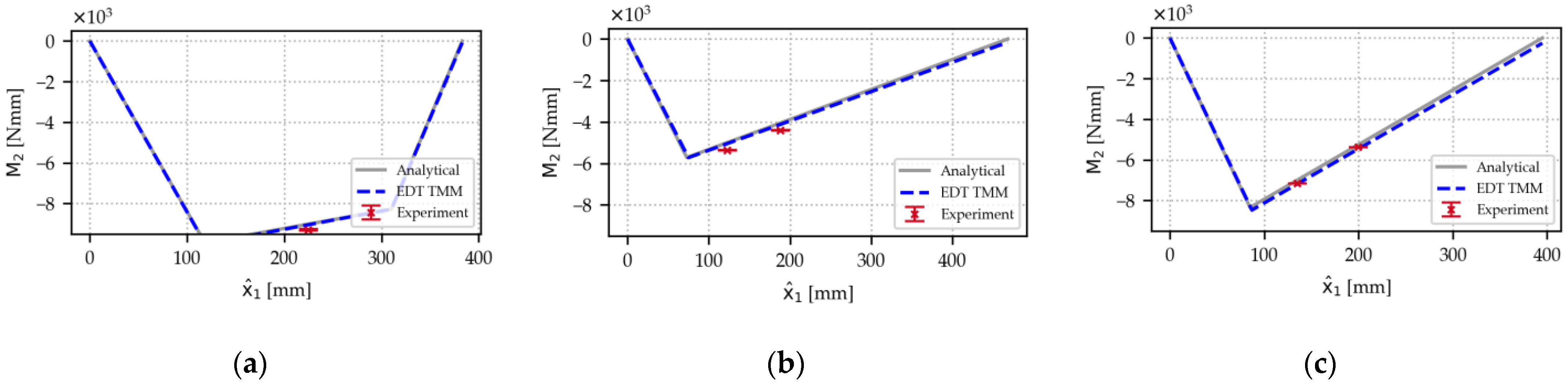
For all beams, static results for bending moments about the ${\widehat{\mathbf{e}}}_2$-axes are plotted in Figure 15 for a direct comparison, showing a good agreement of all three beams of the lab-scale demonstrator. As the experiments were carried out three times, mean values are shown, and the variability is displayed through error bars from minimum to maximum measured values; overall, the variability in the experiments is very small. The figure shows results for a maximum actuator stroke of 100 mm; at actuator strokes of 28 mm and 64 mm, all results showed similar behavior (see Figure A1 and Figure A2). A negative bending moment dominates over the entire length, as we see compression on bottom webs and tension on top webs. The bending moment is zero at hinged supports and free ends. Bending moments reach a peak at hinge joints to other parts of the structure. The results for the EDT TMM solution and the analytical solution match almost exactly. This behavior was expected, as the TMM is an implementation of the analytical solution. The negligible difference is a discretization error, as in our implementation, hinge forces are introduced at the nearest cross-section and not in the middle of a beam interval. A comparison with experimental results reveals a high degree of agreement between simulated and experimental bending moments at all five positions of strain gauges. This indicates that the TMM accurately captures section forces and moments in static EDT scenarios.

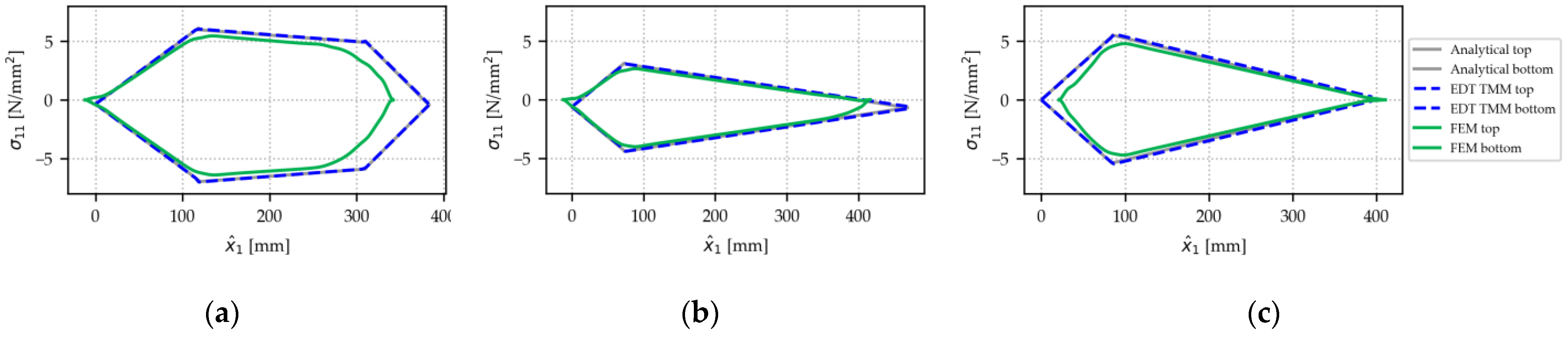
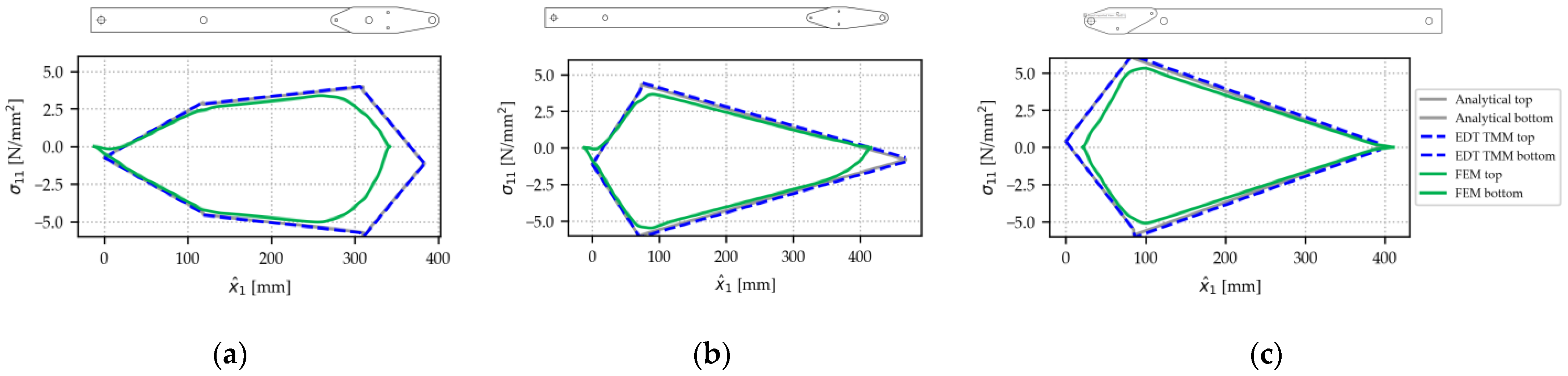
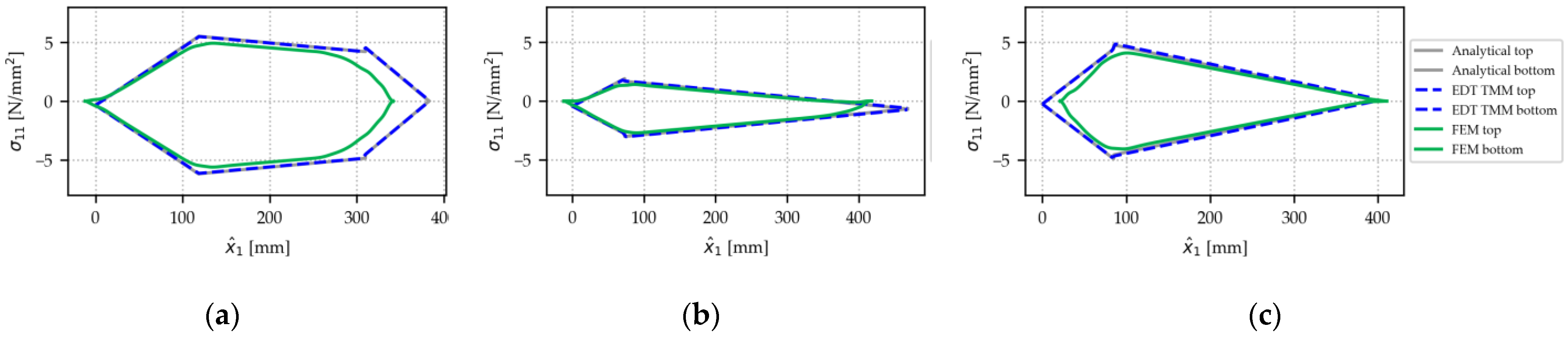
For all beams, static results for normal stresses in the ${\widehat{\mathbf{e}}}_1$-direction are plotted in Figure 16. Stresses are shown for the top and bottom webs of all beams. Again, the figure shows results for a maximum actuator stroke of 100 mm; at actuator strokes of 28 mm and 64 mm, all results revealed similar behavior (Figure A3 and Figure A4). Comparison with the numerical FEM model shows a high degree of agreement along most parts of the beam but with some deviations observed in close proximity to load introduction points, such as hinge joints. In order to facilitate the interpretation of the results, sketches of all beams, including the respective connecting elements, are shown above each plot.

The deviations between the FEM model, on the one hand, and the analytical model and EDT TMM, on the other hand, are caused by an abstraction inherent in all analytical beam implementations; the beams of the lab-scale demonstrator are implemented as having a continuous cross-section and running exactly from the first to the last joint. Consequently, this simplification neglects some details, such as linking elements, as well as holes for the hinge joints. These details are present only in our FEM model, which provides us with locally resolved stresses at load introduction points. At linking elements, the FEM also shows the effect of these elements on stresses in the beam webs, while the analytical models and the EDT TMM ignore this effect. The analysis of normal stresses highlights both the good agreement of the EDT TMM implementation with established methods, as well as its limitations when it comes to reflecting local stress distribution around complex load introduction points. The consequences of this behavior are further discussed in the next section.

4.3.2. Dynamic Results

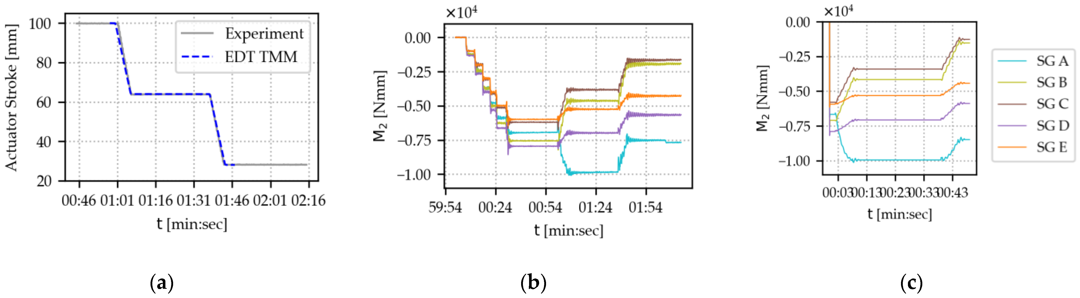
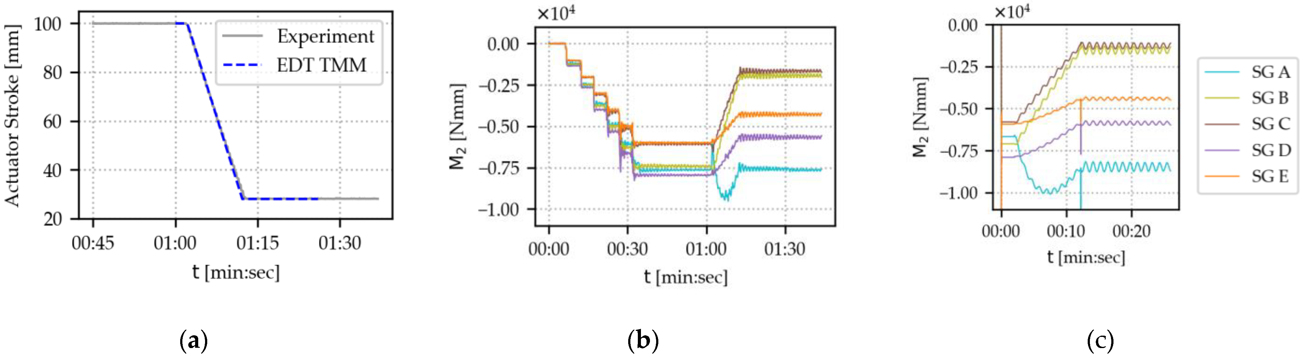
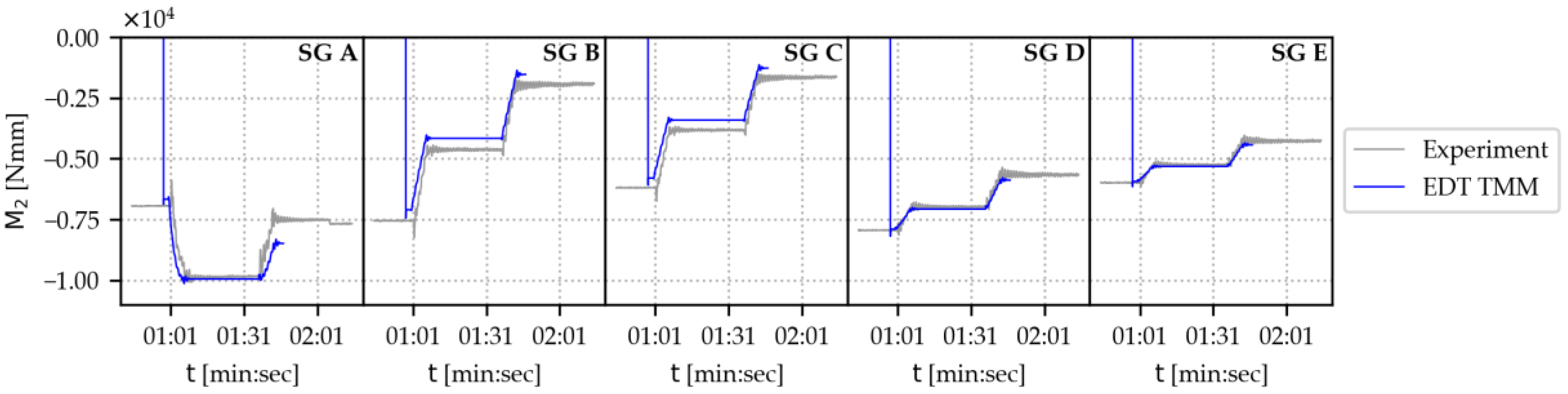
Figure 17 shows results for bending moments about ${\widehat{\mathbf{e}}}_2$-axes at the strain gauge positions, as well as a visualization of the actuator stroke. The plots show a maximum to minimum stroke scenario (100–28 mm); plots for the experiment and the corresponding EDT scenario are given. Note that a bending moment of zero is equivalent to the empty bucket load (0.51 kg) at the position of the maximum stroke. The step plot at the start of the experiment shows the initial loading with 3.06 kg of water bottles. The actuator movement starts at around 01:00 min after the start of recording and lasts for 12 s. In the actuator stroke plot, the actuator movement of the EDT model has been shifted by one minute, so the moments of the actuator start aligning.

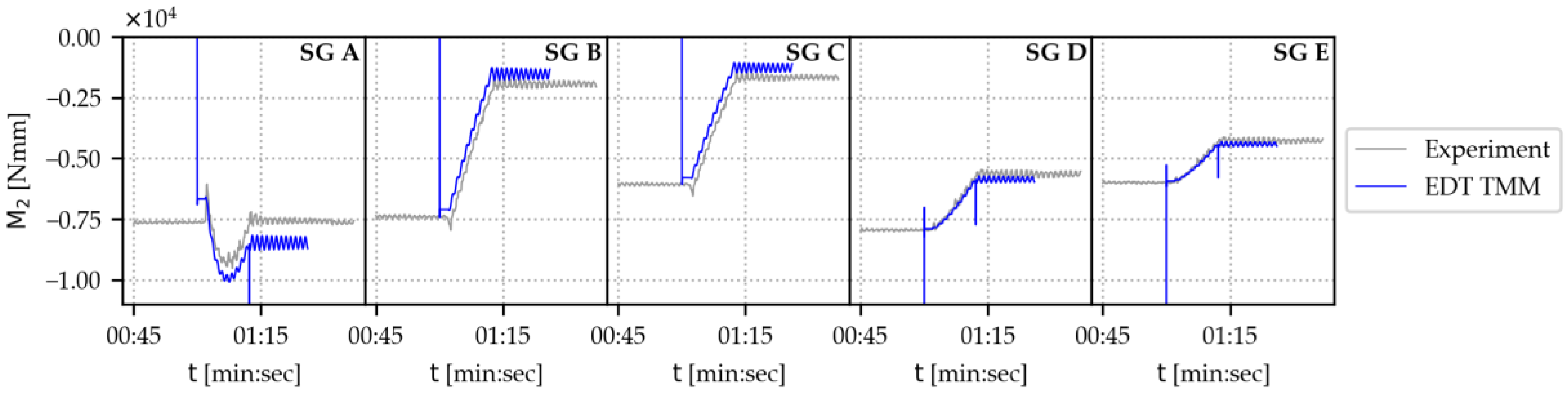
From a qualitative perspective, the plots for the experiment and the EDT TMM seem to agree in Figure 17b,c. The bending moment at strain gauge positions B to E shows an almost linear, decreasing behavior over time, although with varying steepness. The bending moment at position A differs in shape: We see a convex curve with a maximum absolute bending moment at around half the actuator stroke. For a quantitative comparison, we plot the values for the strain gauges and the simulated values in the same plots in Figure 18. Again, the EDT TMM seems to reflect the experiment of the use case very well. We carried out the same analysis for the maximum to half to minimum stroke scenario, which showed a similar, excellent degree of agreement (see Figure A5 and Figure A6).

5. Discussion

We discuss the validation experiments described in Section 3 and Section 4, as well as the limitations of the method that we observed during our studies. Reflecting these benefits and limitations, we discuss potential application scenarios.

Overall, our implementation of the EDT TMM showed excellent agreement with all static and dynamic experiments. It also showed excellent agreement with all static analytical benchmark tests. Deviations when comparing established models existed for Example 6 in Section 3 and when comparing local stresses at load introduction points with the FEM for the use case in Section 4. When it comes to practically applying the EDT TMM in engineering, we consider these kinds of deviations manageable, although engineers must be aware of the effects that cause these deviations. The validation examples showed that the TMM is a suitable tool for investigating forces, moments, and torques acting within a system using an EDT.

We want to point out three main limitations when using the EDT TMM; they also include the reasons for the above-described deviations:

• Limited performance in dynamic scenarios with high accelerations;
• Limited local resolution;
• Use in statically determinate systems only.

The last two points were expected; as the TMM is an implementation of the analytical solution of equilibrium equations of a single Bernoulli beam, it cannot exceed the capabilities of the original analytical solution. Therefore, it cannot represent local stresses around holes and other points of discontinuity. Although feasible in principle, an expansion of the TMM to statically indeterminate systems would be a much more complex challenge, requiring the consideration of stiffnesses and deformations; deformations are not calculated in the present approach. Therefore, it was not considered in this study to keep the focus on the integration into an EDT on a system level.

The first point, limited performance in highly dynamic scenarios, is a consequence of how inertia forces are calculated; as the inertia forces are calculated from the accelerations, their accuracy highly depends on the acceleration accuracy. As the acceleration is calculated over a finite step length of the RBD, a step length that is chosen too long results in a low accuracy of inertia forces. These inaccuracies build up over the beam length since transfer matrices with small deviations are multiplied. It is the engineer’s responsibility to ensure a reasonable trade-off between accuracy (smaller time steps better) and computational speed (larger time steps better) for dynamic scenarios.

Overall, the limitations confirm what also holds for any other model or process in engineering design; it is the users’ responsibility to ensure that their model is suitable for the specific purpose. In particular, that means that the EDT TMM is only applicable where the EDT’s RBD is applicable since the TMM relies on the RBD results. As such, its application is limited to scenarios where structural flexibility can be disregarded. Examples of where the combination of EDT RBD and TMM is not a good choice for force simulation include elements of a truss bridge (as this is usually a statically indeterminate system), a connector shaft in a piston engine (as high accelerations are involved), or systems that require an analysis of vibrational modes (as deformations are non-negligible). When aware of these limitations, the EDT TMM can be a useful tool for engineers.

So, what would be a suitable application for the EDT with a TMM-based force and stress simulation? We believe the capability to operate within a simulation on a system level is where the strength of the approach lies. Engineers could benefit from this as follows:

• Improved load assessment in the early engineering design process. In EDTs acting as virtual prototypes, load assumptions can be derived from simulations of entire systems in virtual scenarios;
• Parametric studies on a system level and thus for optimization on a system level, e.g., by assessing the impact of control parameters on beam loads;
• Detection of unforeseen and undesirable behavior, e.g., by combining stress calculations with fatigue estimation algorithms.

Industries that could benefit are all those with high operational complexity and uncertain loading conditions, e.g., heavy equipment manufacturers in construction, agricultural engineering, and plant engineering.

A concern that will arise when scaling the approach to these more complex applications is the demand for additional computational resources that the coupling of EDT and TMM will create. Until today, all computations have been performed on standard computers. As the TMM works continuously along the model, computational resources and time should be growing with order O(N) regarding the number of structural elements. During preliminary tests conducted by the authors on more complex models, i.e., load cases for several parts of a forestry machine, computational resources did not pose a problem. Nonetheless, more research on the computational performance of our approach for statically determinate systems of higher complexity is needed to support this assumption.

All the above-described applications for EDT TMM have in common that they do not replace current well-established methods of structural analysis but rather amend them to gain insights at a different stage of the engineering design process. Future research should focus on systematically exploring how EDT can be effectively integrated into existing structural design workflows.

6. Conclusions

This paper presented investigations on the transfer matrix method (TMM) as a tool to simulate forces and stresses for statically determinate beam structures in Experimentable Digital Twins (EDT), with a focus on its abilities in system-level simulations. The authors implemented a coupling between rigid body dynamics (RBD) and TMM into an existing EDT framework. In separated scenarios that were chosen to be verifiable by straightforward analytical calculations, we validated the ability of the TMM to handle concentrated, gravitational, and inertia forces in static and dynamic scenarios.

In static and dynamic experiments, a lab-scale demonstrator represented a system with an actuator and a multi-beam mechanism as an example use case. Investigations of an EDT for this use case system and a comparison of results of the TMM implementation against a numerical model and experimental strain measurements revealed the TMM’s ability to accurately reflect forces and stresses in beams in system-level scenarios.

The discussion section highlights potential application scenarios and limitations for force and stress simulations in EDT using the TMM. Potential application scenarios include load estimations in virtual prototypes of systems, optimization on a system level, and detection of unforeseen and undesirable behavior. Among the limitations of our approach are a limited performance in highly dynamic scenarios, a coarse resolution of stresses unsuitable for local phenomena, and the limitation to statically determinate systems. Co-simulation of detailed structural simulations and other physical simulations remains a major challenge in industry and academia, and our contribution is intended to be a helpful tool for certain engineering applications on a system level.

The findings discussed in this paper provide a strong basis for further exploration, and the authors are optimistic that the insights achieved will contribute to future developments in simulation-based engineering. Future upgrades to the EDT framework can include a direct usage of TMM results in further calculations on runtime, e.g., by combining it with tools for notch concentration factors and fatigue estimation. Future academic research should aim to investigate ways to seamlessly incorporate EDT into established structural design processes.

References

- Schluse, M.; Priggemeyer, M.; Atorf, L.; Rossmann, J. Experimentable Digital Twins—Streamlining Simulation-Based Systems Engineering for Industry 4.0. IEEE Trans. Ind. Inf. 2018, 14, 1722–1731. [Google Scholar] [CrossRef]
- Busch, M. Zur Effizienten Kopplung von Simulationsprogrammen/Martin Busch; Kassel University Press: Kassel, Germany, 2012; ISBN 9783862192977. [Google Scholar]
- Gomes, C.; Thule, C.; Broman, D.; Larsen, P.G.; Vangheluwe, H. Co-Simulation: State of the Art; CoRR, Cornell University Library, Ithaca, NY, USA: 2017. [CrossRef]
- Stettinger, G.; Benedikt, M.; Thek, N.; Zehetner, J. On the difficulities of real-time co-simulation. In Proceedings of the V International Conference on Computational Methods for Coupled Problems in Science and Engineering, Ibiza, Spain, 17–19 June 2013; pp. 989–999. [Google Scholar]
- Schmoll, R. Co-Simulation und Solverkopplung: Analyse Komplexer Multiphysikalischer Systeme. Ph.D. Dissertation, Kassel University Press, Kassel, Germany, 2015. [Google Scholar]
- Largilliere, F.; Verona, V.; Coevoet, E.; Sanz-Lopez, M.; Dequidt, J.; Duriez, C. Real-time control of soft-robots using asynchronous finite element modeling. In Proceedings of the 2015 IEEE International Conference on Robotics and Automation (ICRA), Seattle, WA, USA, 26–30 May 2015; pp. 2550–2555. [Google Scholar]
- Frank, B.; Stachniss, C.; Schmedding, R.; Teschner, M.; Burgard, W. Learning object deformation models for robot motion planning. Robot. Auton. Syst. 2014, 62, 1153–1174. [Google Scholar] [CrossRef]
- MpCCI. Available online: https://www.mpcci.de/ (accessed on 9 December 2024).
- Ansys Mechanical. Available online: https://www.ansys.com/products/structures/ansys-mechanical (accessed on 9 December 2024).
- Zwölfer, A.; Gerstmayr, J. A concise nodal-based derivation of the floating frame of reference formulation for displacement-based solid finite elements. Multibody Syst. Dyn. 2020, 49, 291–313. [Google Scholar] [CrossRef]
- Chung, G.-J.; Kim, D.-H.; Shin, H.; Ko, H.-J. Structural analysis of 600Kgf heavy duty handling robot. In Proceedings of the 2010 IEEE Conference on Robotics, Automation and Mechatronics, Singapore, 27–29 June 2010; IEEE: Piscataway, NY, USA, 2010; pp. 40–45, ISBN 978-1-4244-6503-3. [Google Scholar]
- Kono, D.; Lorenzer, T.; Weikert, S.; Wegener, K. Comparison of Rigid Body Mechanics and Finite Element Method for Machine Tool Evaluation D. Kono [und weitere]; Eidgenössische Technische Hochschule Zürich, Institut für Werkzeugmaschinen und Fertigung: Zürich, Switzerland, 2010. [Google Scholar]
- Wang, X.; Mills, J.K. A FEM model for active vibration control of flexible linkages. In Proceedings of the IEEE International Conference on Robotics and Automation, New Orleans, LA, USA, 25–30 April 2004; IEEE: Piscataway, NY, USA, 2004; Volume 5, pp. 4308–4313, ISBN 0-7803-8232-3. [Google Scholar]
- Dietz, S.; Hippmann, G.; Schupp, G. Interaction of Vehicles and Flexible Tracks by Co-Simulation of Multibody Vehicle Systems and Finite Element Track Models. Veh. Syst. Dyn. 2002, 37, 372–384. [Google Scholar] [CrossRef]
- Haag, S.; Anderl, R. Digital twin—Proof of concept. Manuf. Lett. 2018, 15, 64–66. [Google Scholar] [CrossRef]
- Lai, X.; He, X.; Wang, S.; Wang, X.; Sun, W.; Song, X. Building a Lightweight Digital Twin of a Crane Boom for Structural Safety Monitoring Based on a Multifidelity Surrogate Model. J. Mech. Des. 2022, 144, 064502. [Google Scholar] [CrossRef]
- Integrate Deformable Components’ Behavior into a Real-Time Capable Overall System Simulation for Robotics. In Proceedings of the 2018 IEEE/ASME International Conference on Advanced Intelligent Mechatronics (AIM), Auckland, New Zealand, 8–11 July 2018; IEEE: Piscataway, NY, USA, 2018; pp. 1384–1389, ISBN 978-1-5386-1854-7.
- Kaufmann, D.; Rossmann, J. Integration of structural simulations into a real-time capable Overall System Simulation for complex mechatronic systems. Int. J. Model. Simul. Sci. Comput. 2019, 10, 1940002. [Google Scholar] [CrossRef]
- Kaufmann, D.; Rast, M.; Roßmann, J. Implementing a New Approach for Bidirectional Interaction between a Real-time Capable Overall System Simulation and Structural Simulations—Completion of the Virtual Testbed with Finite Element Analysis. In Proceedings of the 7th International Conference on Simulation and Modeling Methodologies, Technologies and Applications, Madrid, Spain, 26–28 July 2017; SCITEPRESS—Science and Technology Publications: Setúbal, Portugal, 2017; pp. 114–125, ISBN 978-989-758-265-3. [Google Scholar]
- Rossmann, J.; Stern, O.; Kupetz, A.; Jochmann, G.; Schluse, M.; Kaufmann, D.; Dahmen, U.; Wahl, A.; Thieling, J.; Osterloh, T. The Virtual Testbed Approach towards Modular Satellite Systems. In Proceedings of the 69th International Astronautical Congress, Bremen, Germany, 1–5 October 2018; pp. 1–5. [Google Scholar]
- Kaufmann, D.; Roßmann, J. Finite Element Analysis as a Key Functionality for eRobotics to Predict the Interdependencies between Robot Control and Structural Deformation. In Tagungsband des 3. Kongresses Montage Handhabung Industrieroboter; Schüppstuhl, T., Tracht, K., Franke, J., Eds.; Springer: Berlin/Heidelberg, Germany, 2018; pp. 103–110. ISBN 978-3-662-56713-5. [Google Scholar]
- Krause, M.; Schröder, K.-U.; Kaufmann, D.; Osterloh, T.; Rossmann, J. Coupling of rigid body dynamics with structural mechanics to include elastic deformations in a real-time capable holistic simulation for digital twins. In Modelling and Simulation 2018, Proceedings of the European Simulation and Modelling Conference 2018, Ghent, Belgium, 24–26 October 2018; Limere, V., Claeys, D., Eds.; EUROSIS: Ostend, Belgium, 2018; ISBN 978-949285905-1. [Google Scholar]
- Schmid, S.; Dahmen, U.; Shao, L.; Schroder, K.-U.; Rossmann, J. Developing an experimentable digital twin of a novel forestry machine: Application, experiences, and benefits. In Proceedings of the 14th International Workshop on Structural Health Monitoring, Stanford, CA, USA, 12–14 September 2023; Destech Publications, Inc.: Lancaster, PA, USA, 2023. ISBN 9781605956930. [Google Scholar]
- Grieves, M. Digital Twin: Manufacturing Excellence through Virtual Factory Replication. White Pap. 2014. [Google Scholar]
- Shafto, M.; Conroy, M.; Doyle, R.; Glaessgen, E.; Kemp, C.; LeMoigne, J.; Wang, L. Modeling, Simulation, Information Technology and Processing Roadmap: Technology Area 11; NASA (National Aeronautics and Space Administration): Washington, DC, USA, 2010. [Google Scholar]
- Negri, E.; Fumagalli, L.; Macchi, M. A Review of the Roles of Digital Twin in CPS-based Production Systems. Procedia Manuf. 2017, 11, 939–948. [Google Scholar] [CrossRef]
- Panetta, K. Trends in the Gartner Hype Cycle for Emerging Technologies, 2018. Available online: www.gartner.com/smarterwithgartner/5-trends-emerge-in-gartner-hype-cycle-for-emerging-technologies-2018 (accessed on 3 March 2019).
- Gašpar, T.; Deniša, M.; Radanovič, P.; Ridge, B.; Savarimuthu, T.R.; Kramberger, A.; Priggemeyer, M.; Roßmann, J.; Wörgötter, F.; Ivanovska, T.; et al. Smart hardware integration with advanced robot programming technologies for efficient reconfiguration of robot workcells. Robot. Comput. -Integr. Manuf. 2020, 66, 101979. [Google Scholar] [CrossRef]
- Baidya, S.; Das, S.K.; Uddin, M.H.; Kosek, C.; Summers, C. Digital Twin in Safety-Critical Robotics Applications: Opportunities and Challenges. In Proceedings of the 2022 IEEE International Performance, Computing, and Communications Conference (IPCCC), Austin, TX, USA, 10–12 November 2022; IEEE: Piscataway, NY, USA, 2022; pp. 101–107, ISBN 978-1-6654-8018-5. [Google Scholar]
- Wang, T.; Feng, K.; Ling, J.; Liao, M.; Yang, C.; Neubeck, R.; Liu, Z. Pipeline condition monitoring towards digital twin system: A case study. J. Manuf. Syst. 2024, 73, 256–274. [Google Scholar] [CrossRef]
- Liao, M.; Renaud, G.; Bombardier, Y. Airframe digital twin technology adaptability assessment and technology demonstration. Eng. Fract. Mech. 2020, 225, 106793. [Google Scholar] [CrossRef]
- Rast, M. Domänenübergreifende Modellierung und Simulation als Grundlage für Virtuelle Testbeds, 1st ed. Ph.D. Dissertation, Edition Wissenschaft, Apprimus, Aachen, Germany, 2014. [Google Scholar]
- Rossmann, J.; Schluse, M. Virtual Robotic Testbeds: A Foundation for e-Robotics in Space, in Industry—And in the Woods. In Proceedings of the 2011 Developments in E-systems Engineering (DeSE), Dubai, United Arab Emirates, 5–7 December 2011; IEEE: Piscataway, NY, USA, 2011; pp. 496–501, ISBN 978-1-4577-2186-1. [Google Scholar]
- Schluse, M. Experimentierbare Digitale Zwillinge; Springer Fachmedien Wiesbaden: Wiesbaden, Germany, 2024; ISBN 978-3-658-44444-0. [Google Scholar]
- Dassault Systemes, Simulia. Available online: https://www.3ds.com/products/simulia (accessed on 9 December 2024).
- Hexagon Adams. Available online: https://hexagon.com/products/product-groups/computer-aided-engineering-software/adams (accessed on 9 December 2024).
- Fließbach, T. Mechanik: Lehrbuch zur Theoretischen Physik I; Springer: Berlin/Heidelberg, Germany, 2020; ISBN 978-3-662-61602-4. [Google Scholar]
- Jung, T.J. Methoden der Mehrkörperdynamiksimulation als Grundlage Realitätsnaher Virtueller Welten, 1st ed.; Aachen, Techn. Hochsch., Ph.D. Dissertation, 2011; Verlag Dr. Hut: München, Germany, 2011; ISBN 3843901511. [Google Scholar]
- Köstner, H. Strukturmechanische Berechnungen Mittels Übertragungsmatrizen am Beispiel von Schalen. Ph.D. Dissertation, RWTH Aachen University, Aachen, Germany, 1990. [Google Scholar]
- Rittweger, A. Statik, Stabilität und Eigenschwingungen Anisotroper Rotationsschalen Beliebigen Meridians mit der Ü bertragungsmatrizen-Methode. Ph.D. Dissertation, Aachen, Technical University, Aachen, Germany, 1992. [Google Scholar]
- Stewart, D.; Trinkle, J.C. An implicit time-stepping scheme for rigid body dynamics with Coulomb friction. In Proceedings of the IEEE International Conference on Robotics and Automation, San Francisco, CA, USA, 24–28 April 2000; IEEE: Washington, DC, USA, 2000; pp. 162–169, ISBN 0-7803-5886-4. [Google Scholar]
- Verosim. Available online: https://www.verosim-solutions.com/ (accessed on 9 December 2024).
Figure 1.
A blend of Experimentable Digital Twin (EDT) for stress visualization and its counterpart, the real-world asset. Photomontage of a screenshot from the EDT framework and a photograph of the lab-scale demonstrator.
Figure 2.
Section forces of a beam interval with length l subject to bending about the -axis.
Figure 3.
Screenshot of an EDT model visualization to highlight the coordinate systems. Section forces are computed in the local -coordinate system of a beam. The global -coordinate system is also shown.
Figure 4.
Validation example for the EDT TMM: A cantilever beam subject to a tip load: (a) Sketch and input quantities. (b) Results: The EDT TMM solution matches the analytical solution.
Figure 5.
Validation example for the EDT TMM: A cantilever beam subject to three concentrated loads: (a) Sketch and input quantities. (b) Results: The EDT TMM solution matches the analytical solution.
Figure 6.
Validation example for the EDT TMM: A cantilever beam under gravity: (a) Sketch and input quantities. The mass corresponds to an aluminum beam. (b) Results: The EDT TMM solution matches the analytical solution.
Figure 7.
Validation example for the EDT TMM: A cantilever beam with a rotating tip mass: (a) Sketch and input quantities. (b) Results: Section moment about -axis plotted at three points along the beam axis. The TMM matches the analytical solution. (c) Section moment about -axis. EDT TMM solution plotted along the entire beam’s length to demonstrate the capabilities to handle skewed bending.
Figure 8.
Validation example for the EDT TMM: A rotating beam. (a) Sketch and input quantities. The mass corresponds to an aluminum beam. (b) Results: The TMM matches the analytical solution.
Figure 9.
Validation example for the EDT TMM: A beam falling under gravity. (a) Sketch and input quantities. (b) Results: The TMM matches the analytical solution at the position of maximum bending moment but diverges towards the free end of the beam.
Figure 10.
Example use case for validation purposes: (a) Lab-scale demonstrator used for experiments. (b) Experimentable Digital Twin showing stress visualization. (c) Finite-Element-Model. (d) Two-dimensional analytical model.
Figure 11.
The lab-scale use case demonstrator is a mechanism with one degree of freedom. (a) Cross-section of aluminum beams. (b) Box cross-section using middle-line approximation for analytical and TMM implementation. (c) Overview of the lab-scale demonstrator with an indication of strain gauge positions (A–E) and load introduction.
Figure 12.
Definition of the components (beams, links, rods, base, actuator) and axes (A1 to A12) in the mechanical design of the laboratory demonstrator.
Figure 13.
Model topology of the EDT in the simulation domain of rigid-body dynamics. Red lines represent passive joint connections, green dotted lines represent actuated joint connections.
Figure 14.
Kinematic workspace of the laboratory demonstrator. The TCP can only be moved along the red line in the x–z plane.
Figure 15.
Bending moment about the about -axis for the three beams of the example use case. The experimental values show the means and total range of measured values for three experiments. Taken at maximum actuator stroke (100 mm) and 30 N load. (a) Beam 1. (b) Beam 2. (c) Beam 3.
Figure 16.
Stresses along the top and bottom webs for the three beams of the example use case. Top webs are under tension in this load case. Taken at maximum actuator stroke (100 mm) and 30 N load. Side views are shown on top. (a) Beam 1. (b) Beam 2. (c) Beam 3.
Figure 17.
Bending moments at strain gauge positions for the three beams of the lab-scale demonstrator use case. Taken from a dynamic scenario, running from maximum to minimum actuator stroke (100–28 mm) and 30 N load. (a) Actuator stroke comparison, EDT TMM stroke shifted by 1 min. (b) Experimental results (c) EDT TMM results.
Figure 18.
Bending moments about the -axis over time for all strain gauges and their respective positions in the dynamic EDT scenario of the example use case. The scenario represents an actuator movement from maximum actuator stroke (100 mm) to minimum actuator stroke (28 mm), with a weight of 3.57 kg at the tip. From left to right:Beam 1, strain gauge A. Beam 2, strain gauge B. Beam 2, strain gauge C. Beam 3, strain gauge D. Beam 3, strain gauge E.