Influence of Panel Zone Modeling on the Seismic Behavior of Steel Moment-Resisting Frames: A Numerical Study

Abstract

In the seismic design of steel moment-resisting frames (MRFs), the panel zone region can significantly affect overall ductility and energy-dissipation capacity. This study investigates the influence of panel zone flexibility on the seismic response of steel MRFs by comparing two modeling approaches: one with a detailed panel zone representation and the other considering fixed beam-column connections. A total of 30 2D steel MRFs (15 frames incorporating panel zone modeling and 15 frames without panel zone modeling) are subjected to nonlinear time–history analyses using four suites of ground motions compatible with Eurocode 8 (EC8) soil types (A, B, C, and D). Structural performance is evaluated at three distinct performance levels, namely, damage limitation (DL), life safety (LS), and collapse prevention (CP), to capture a wide range of potential damage scenarios. Based on these analyses, the study provides information about the seismic response of these frames. Also, lower-bound, upper-bound, and mean values of behavior factor (q) for each soil type and performance level are displayed, offering insight into how panel zone flexibility can alter a frame’s inelastic response under seismic loading. The results indicate that neglecting panel zone action leads to an artificial increase in frame stiffness, resulting in higher base shear estimates and an overestimation of the seismic behavior factor. This unrealistically increased behavior factor can compromise the accuracy of the seismic design, even though it appears conservative. In contrast, including panel zone flexibility provides a more realistic depiction of how forces and deformations develop across the structure. Consequently, proper modeling of the panel zone supports both safety and cost-effectiveness under strong earthquake events.

1. Introduction

The panel zone in a steel moment-resisting frame (MRF) refers to the segment of the column web enclosed by the column flanges and, if present, continuity plates at the beam-column intersection [1,2,3]. This confined but essential region is critical for resisting shear forces transferred from beams to columns and can undergo significant inelastic deformations during seismic events. As such, the panel zone contributes significantly to providing ductility and dissipating seismic energy [4,5,6].

Achieving the right balance between panel zone strength and flexibility is crucial to ensure effective seismic energy dissipation while avoiding detrimental impacts on global structural performance [7,8,9]. Excessively stiff panel zones can transfer high inelastic demands to beams, increasing the risk of brittle failures, while excessively flexible panel zones may lead to large inter-story drifts and substantially reduced lateral stiffness [10,11,12]. Thus, accurate modeling and thoughtful design of panel zones are essential to maintaining both the strength and ductility of steel MRFs under seismic loading [13,14,15].

In terms of analytical representation, one of the most common and simple strategies for capturing panel zone deformations is the “scissors model”, which idealizes the panel zone as a single rotational spring reflecting shear flexibility. More advanced methods account for the simultaneous effects of shear, bending, and even axial forces, trying to better simulate the true inelastic mechanisms that occur in practice, which are described in Refs. [4,11,12,14,15]. For instance, quadri-linear and multi-spring models have been proposed to capture both elastic and inelastic regions of deformation, incorporating strain-hardening behaviors and geometric constraints [12,15]. Others extend these approaches to include axial stress interactions on thick flanges, ensuring that panel zone demands remain consistent with beam and column design assumptions [11]. Such models facilitate more accurate predictions of story drifts, shear demands, and energy dissipation, ultimately enabling a more reliable assessment of steel MRF performance under seismic loading [4,14].

Recent investigations highlight that neglecting the panel zone (PZ) deformations can lead to inaccurate design outcomes in steel MRFs [16,17,18,19]. For example, Isaincu et al. [16] showed that disregarding panel zone flexibility can significantly overestimate second-order effects, potentially compromising safety margins. Rigi et al. [17] highlighted that semi-rigid connections exhibit improved energy dissipation when the panel zone is modeled accurately, while Sepasdar et al. [18] found that strong panel zones do not always alter the global structural response significantly. Lu et al. [19] show that reinforcing the panel zone with a box section effectively improves seismic performance, reduces inter-story drift, and minimizes the risk of brittle fractures in steel special moment frames (SMFs). Tuna and Topkaya [20] similarly demonstrated how discrepancies in design standards yield considerable variance in panel zone-yielding demands. Furthermore, prior research on panel zone behavior [1] has shown that steel MRFs experience significant shear and rotational demands in the beam-column joints during strong ground motions, leading to considerable inelastic panel zone deformation. In contrast, braced frames, due to their higher overall stiffness and reduced interstory drifts, exhibit less significant panel zone rotations. As a result, analyzing MRFs allows for a clearer assessment of the panel zone’s role, particularly in capturing inelastic rotations, their impact on drift, and plastic mechanism formation. Overall, these findings highlight the importance of robust panel zone modeling for advanced seismic analysis and performance-based design in steel MRFs.

This study employs the simplicity and demonstrated effectiveness of the “scissors model” to accurately capture in-plane shear deformations within the panel zone region. Specifically, this research investigates the impact of panel zone flexibility on the global seismic performance of steel MRFs by analyzing multiple response parameters. The influence of panel zone flexibility on modal characteristics is assessed, with a focus on variations in natural periods. Additionally, the study examines how panel zone deformations affect base shear demands across three distinct performance levels: damage limitation (DL), life safety (LS), and collapse prevention (CP). Table 6 correlates these performance levels with specific damage levels, as defined by [21]. These findings highlight the corresponding strength requirements at various stages of inelastic behavior. The analysis further evaluates changes in lateral stiffness and overall damage potential by investigating the maximum interstory drift ratio (IDR). Finally, the effect of panel zone deformations on the seismic behavior factor is explored, particularly in relation to the above performance levels, to determine how panel zone flexibility may enhance or compromise ductility and energy dissipation capabilities in steel MRFs. The innovative aspect of this study lies in its detailed quantification of how panel zone flexibility affects key seismic response parameters of steel MRFs. While previous research has recognized the influence of panel zone behavior, this study provides a deeper understanding by systematically examining how different performance levels and soil conditions impact the overall structural response.

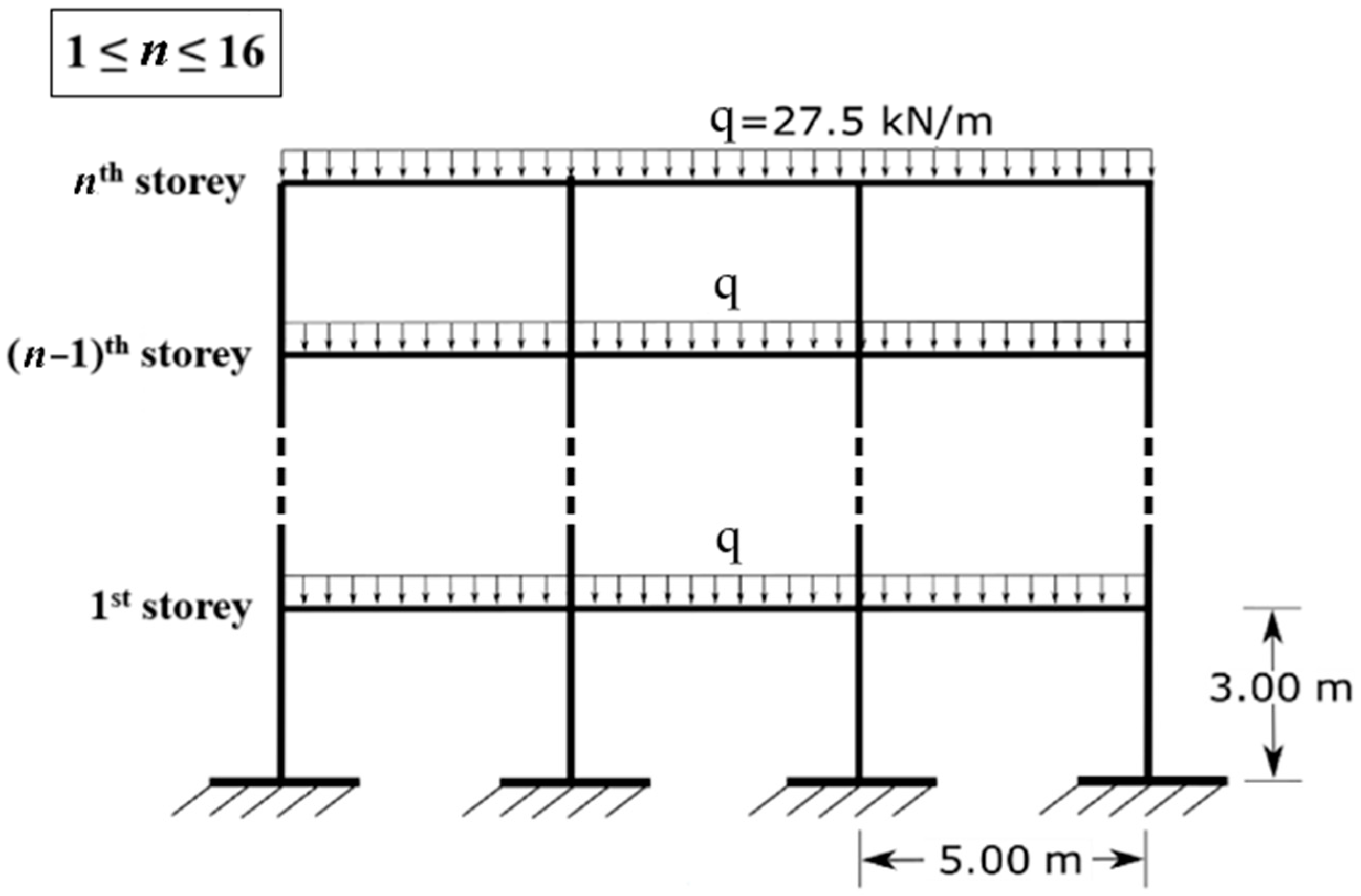
2. Design and Modeling of the Steel MRFs

2.1. Seismic Design of Frames

The steel structures investigated in this study include 15 planar, regular, and orthogonal moment-resisting frames (MRFs) with heights ranging from 2 up to 16 storeys. Each frame retains a uniform storey height of 3.0 m, a bay width of 5.0 m, and three bays in total, as illustrated in Figure 1. Initially, the cross-sectional dimensions of frame members were determined using a seismic design procedure. The design of these MRFs followed the provisions of EC8 [22] and EC3 [23] using SAP2000 software [24]. The gravity load combination G + 0.3Q, combining uniformly distributed dead (G) and live (Q) loads, is considered equal to 27.5 kN/m (Figure 1). Steel grade S275 is employed in the design. The peak ground acceleration (PGA) is 0.24 g for soil type B, with a behavior factor q = 4, corresponding to frames classified as medium ductility class (DCM). Columns employ HEB sections, while beams use IPE sections, with column sections oriented such that their strong axis is perpendicular to the plane of the frame.

Table 1. Summary of steel member sections (columns and beams) used in the MRFs following seismic design.

Frame	Story	Frame Sections HEB (Columns)—IPE (Beams)	T1, no PZ (s)	T2, no PZ (s)	T1, with PZ (s)	T2, with PZ (s)
1	2	400-300 (1), 360-270 (2)	0.343	0.08	0.37	0.08
2	3	400-300 (1), 360-270 (2–3)	0.564	0.14	0.611	0.15
3	4	400-300 (1–2), 360-270 (3–4)	0.758	0.21	0.832	0.22
4	5	400-300 (1–2), 360-270 (3–5)	0.996	0.29	1.099	0.31
5	6	400-300 (1–3), 360-270 (4–6)	1.196	0.36	1.328	0.39
6	7	450-330 (1), 400-300 (2–4), 360-270 (5–7)	1.350	0.42	1.516	0.46
7	8	450-330 (1), 400-300 (2–4), 360-270 (5–8)	1.597	0.51	1.787	0.55
8	9	450-330 (1–2), 400-300 (3–5), 360-270 (6–9)	1.762	0.57	1.982	0.63
9	10	450-330 (1–3), 400-300 (4–6), 360-270 (7–10)	1.919	0.64	2.169	0.71
10	11	450-330 (1–4), 400-300 (5–7), 360-270 (8–11)	2.075	0.71	2.354	0.78
11	12	500-360 (1), 450-330 (2–5), 400-300 (6–8), 360-270 (9–12)	2.202	0.76	2.505	0.84
12	13	500-360 (1–2), 450-330 (3–6), 400-300 (7–9), 360-270 (10–13)	2.331	0.81	2.662	0.91
13	14	500-360 (1–3), 450-330 (4–7), 400-300 (8–10), 360-270 (11–14)	2.463	0.87	2.820	0.97
14	15	550-400 (1–2), 500-360 (3–5), 450-330 (6–8), 400-300 (9–11), 360-270 (12–15)	2.496	0.89	2.867	1.00
15	16	550-400 (1–4), 500-360 (5–7), 450-330 (8–10), 400-300 (11–13), 360-270 (14–16)	2.476	0.9	2.861	1.02

provides details of the member sections. For clarity, in Table 1, the column sections (HEB) are listed to the left of the dash, while the beam sections (IPE) are to the right, and storey numbers for these members appear in parenthes.

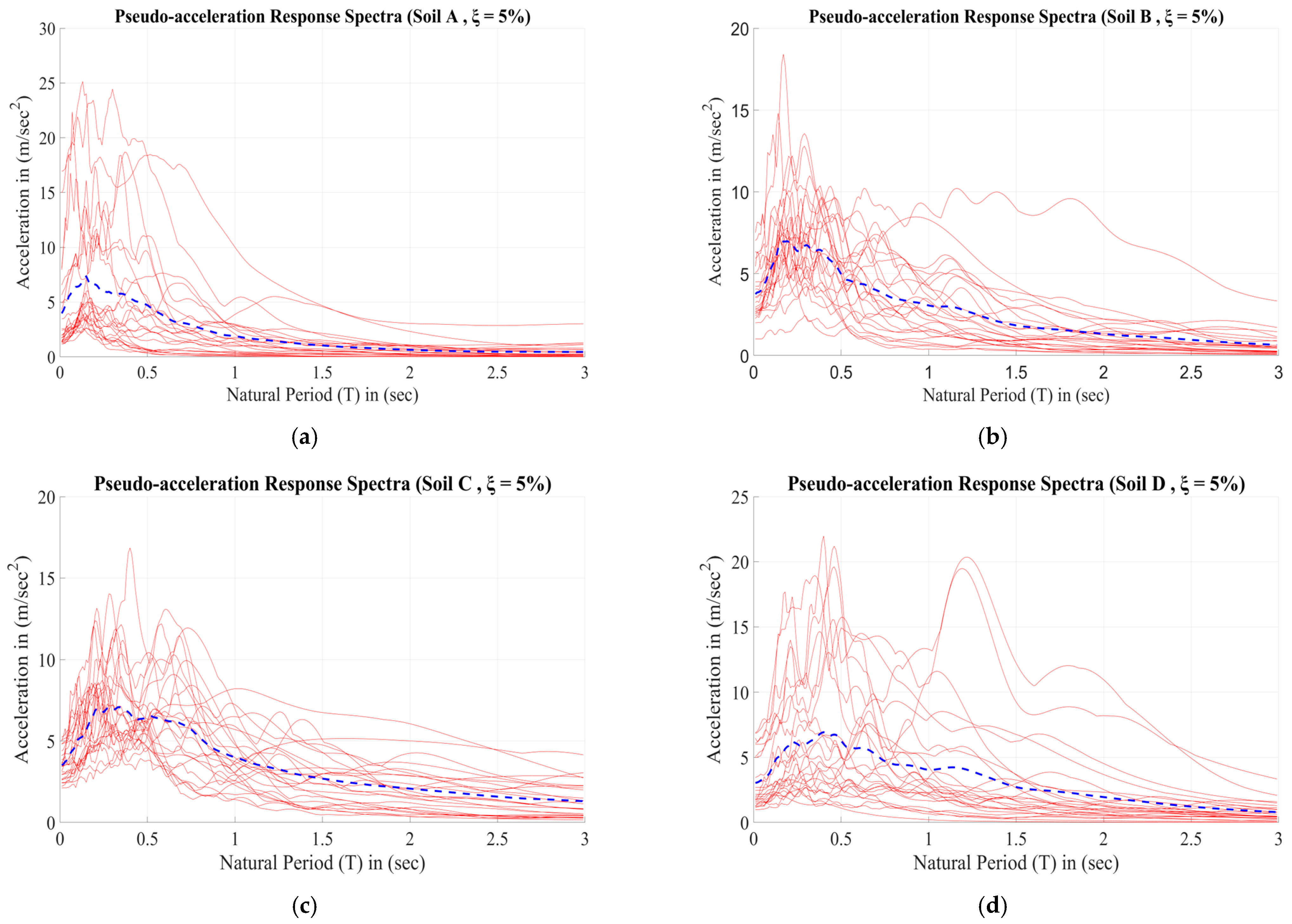
2.2. Seismic Records Considered

A total of 100 far-field seismic recordings are employed for the seismic analyses of the steel MRFs examined in this study. These records, obtained from the PEER (2009) [25] and COSMOS (2013) [26] databases, are categorized into four groups representing soil types A, B, C, and D per EC8 [22].

Table 2. Far-field seismic motions compatible with soil type A.

No.	Date	Record Name	Comp.	Station Name	PGA (g)
1	10/4/1987	Whittier Narrows	NS	24399 Mt Wilson-CIT Station	0.158
2	10/4/1987	Whittier Narrows	EW	24399 Mt Wilson-CIT Station	0.142
3	9/20/1999	Chi-Chi, Taiwan	056-N	HWA056	0.107
4	9/20/1999	Chi-Chi, Taiwan	056-N	HWA056	0.107
5	10/1/1987	Whittier Narrows	NS	24399 Mt Wilson-CIT Station	0.186
6	10/1/1987	Whittier Narrows	EW	24399 Mt Wilson-CIT Station	0.123
7	2/9/1971	San Fernando	N069	127 Lake Hughes 9	0.157
8	2/9/1971	San Fernando	N159	127 Lake Hughes 9	0.134
9	1/17/1994	Northridge	NS	90019 San Gabriel-E. Gr. Ave.	0.256
10	1/17/1994	Northridge	EW	90019 San Gabriel-E. Gr. Ave.	0.141
11	9/20/1999	Chi-Chi, Taiwan	NS	TAP103	0.177
12	9/20/1999	Chi-Chi, Taiwan	EW	TAP103	0.122
13	1/17/1994	Northridge	N005	90017 LA-Wonderland Ave	0.172
14	1/17/1994	Northridge	N175	90017 LA-Wonderland Ave	0.112
15	6/7/1975	Northern Calif.	N060	1249 Cape Mendocino, Petrolia	0.115
16	6/7/1975	Northern Calif.	N150	1249 Cape Mendocino, Petrolia	0.179
17	7/8/1986	N. Palm Springs	NS	12206 Silent Valley	0.139
18	10/18/1989	Loma Prieta	N205	58539 San Francisco	0.105
19	10/18/1989	Loma Prieta	NS	47379 Gilroy Array 1	0.473
20	10/18/1989	Loma Prieta	EW	47379 Gilroy Array 1	0.411
21	8/17/1999	Kocaeli, Turkey	NS	Gebze	0.137
22	8/17/1999	Kocaeli, Turkey	EW	Gebze	0.244
23	6/28/1992	Landers	NS	21081 Amboy	0.115
24	6/28/1992	Landers	EW	21081 Amboy	0.146
25	9/20/1999	Chi-Chi, Taiwan	N034	TCU046	0.133

,

Table 3. Far-field seismic motions compatible with soil type B.

No.	Date	Record Name	Comp.	Station Name	PGA (g)
1	4/25/1992	Cape Mendocino	NS	89509 Eureka	0.154
2	4/25/1992	Cape Mendocino	EW	89509 Eureka	0.178
3	6/9/1980	Victoria, Mexico	N045	6604 Cerro Prieto	0.621
4	6/9/1980	Victoria, Mexico	N135	6604 Cerro Prieto	0.587
5	4/25/1992	Cape Mendocino	EW	89324 Rio Dell Overpass	0.385
6	4/25/1992	Cape Mendocino	NS	89324 Rio Dell Overpass	0.549
7	8/13/1978	Santa Barbara	N048	283 Santa Barbara Courthouse	0.203
8	8/13/1978	Santa Barbara	N138	283 Santa Barbara Courthouse	0.102
9	9/20/1999	Chi-Chi, Taiwan	NS	TCU095	0.712
10	9/20/1999	Chi-Chi, Taiwan	EW	TCU095	0.378
11	8/6/1979	Coyote Lake	N213	1377 San Juan Bautista	0.108
12	8/6/1979	Coyote Lake	N303	1377 San Juan Bautista	0.107
13	1/17/1994	Northridge	NS	90021 LA-N Westmoreland	0.361
14	1/17/1994	Northridge	EW	90021 LA-N Westmoreland	0.401
15	7/8/1986	N. Palm Springs	NS	12204 San Jacinto-Soboba	0.239
16	7/8/1986	N. Palm Springs	EW	12204 San Jacinto-Soboba	0.25
17	9/12/1970	Lytle Creek	N115	290 Wrightwood	0.162
18	9/12/1970	Lytle Creek	N205	290 Wrightwood	0.2
19	10/18/1989	Loma Prieta	NS	58065 Saratoga-Aloha Ave	0.324
20	10/18/1989	Loma Prieta	EW	58065 Saratoga-Aloha Ave	0.512
21	6/28/1992	Landers	NS	22170 Joshua Tree	0.284
22	6/28/1992	Landers	EW	22170 Joshua Tree	0.274
23	9/15/1976	Friuli, Italy	NS	8014 Forgaria Cornino	0.212
24	9/15/1976	Friuli, Italy	EW	8014 Forgaria Cornino	0.26
25	9/20/1999	Chi-Chi, Taiwan	N045	TCU045	0.512

,

Table 4. Far-field seismic motions compatible with soil type C.

No.	Date	Record Name	Comp.	Station Name	PGA (g)
1	9/20/1999	Chi-Chi, Taiwan	NS	NST	0.388
2	9/20/1999	Chi-Chi, Taiwan	EW	NST	0.309
3	5/2/1983	Coalinga	EW	36227 Parkfield	0.147
4	5/2/1983	Coalinga	NS	36227 Parkfield	0.131
5	11/12/1999	Duzce, Turkey	NS	Bolu	0.728
6	11/12/1999	Duzce, Turkey	EW	Bolu	0.822
7	10/15/1979	Imperial Valley	N015	6622 Computertas	0.186
8	10/15/1979	Imperial Valley	N285	6622 Computertas	0.147
9	10/15/1979	Imperial Valley	N012	6621 Chihuahua	0.27
10	10/15/1979	Imperial Valley	N282	6621 Chihuahua	0.284
11	8/17/1999	Kocaeli, Turkey	NS	Atakoy	0.105
12	8/17/1999	Kocaeli, Turkey	EW	Atakoy	0.164
13	10/18/1989	Loma Prieta	NS	1028 Hollister City Hall	0.247
14	10/18/1989	Loma Prieta	EW	1028 Hollister City Hall	0.215
15	4/24/1984	Morgan Hill	NS	57382 Gilroy Array # 4	0.224
16	4/24/1984	Morgan Hill	EW	57382 Gilroy Array # 4	0.348
17	1/17/1994	Northridge	NS	90057 Canyon Country	0.482
18	1/17/1994	Northridge	EW	90057 Canyon Country	0.41
19	2/9/1971	San Fernando	EW	135 LA–Hollywood	0.21
20	2/9/1971	San Fernando	NS	135 LA-Hollywood	0.174
21	4/26/1981	Westmorland	NS	5169 Westmorland Fire Sta	0.368
22	4/26/1981	Westmorland	EW	5169 Westmorland Fire Sta	0.496
23	11/24/1987	Superstition Hills (B)	NS	01335 El Centro Imp. Co. Cent	0.258
24	11/24/1987	Superstition Hills (B)	EW	01335 El Centro Imp. Co. Cent	0.358
25	1/27/1980	Livermore	EW	57187 San Ramon	0.301

and

Table 5. Far-field seismic motions compatible with soil type D.

No.	Date	Record Name	Comp.	Station Name	PGA (g)
1	4/26/1981	Westmorland	N045	5062 Salton Sea Wildlife Ref.	0.199
2	4/26/1981	Westmorland	N135	5062 Salton Sea Wildlife Ref.	0.176
3	11/24/1987	Superstition Hills	N045	5062 Salton Sea Wildlife Refuge	0.119
4	11/24/1987	Superstition Hills	N135	5062 Salton Sea Wildlife Refuge	0.167
5	1/17/1994	Northridge	N064	90011 Montebello-Bluff Rd.	0.128
6	1/17/1994	Northridge	N154	90011 Montebello-Bluff Rd.	0.179
7	10/18/1989	Loma Prieta	NS	58117 Treasure Island	0.159
8	10/18/1989	Loma Prieta	EW	58117 Treasure Island	0.1
9	8/17/1999	Kocaeli, Turkey	NS	Ambarlı	0.184
10	8/17/1999	Kocaeli, Turkey	EW	Ambarlı	0.249
11	10/18/1989	Loma Prieta	N043	1002 APEEL 2-Redwood City	0.274
12	10/18/1989	Loma Prieta	N133	1002 APEEL 2-Redwood City	0.22
13	10/15/1979	Imperial Valley	N040	5057 El Centro Array 3	0.112
14	10/15/1979	Imperial Valley	N130	5057 El Centro Array 3	0.179
15	9/20/1999	Chi-Chi, Taiwan	N041	CHY041	0.639
16	9/20/1999	Chi-Chi, Taiwan	N131	CHY041	0.302
17	10/18/1989	Loma Prieta	N047	1002 APEEL 2-Redwood City	0.274
18	10/18/1989	Loma Prieta	N137	1002 APEEL 2-Redwood City	0.22
19	9/20/1999	Chi-Chi, Taiwan	EW	TAP003	0.126
20	9/20/1999	Chi-Chi, Taiwan	NS	TAP003	0.106
21	1/16/1995	Kobe	NS	Nishi-Akashi	0.503
22	1/16/1995	Kobe	EW	Nishi-Akashi	0.509
23	9/20/1999	Chi-Chi, Taiwan	N040	TCU040	0.123
24	9/20/1999	Chi-Chi, Taiwan	N130	TCU040	0.149
25	1/16/1995	Kobe	NS	Kakogawa	0.345

include these records along with their date, record name, component direction, station, and peak ground acceleration (PGA) value. The 100 records were selected based on two primary criteria: (i) moment magnitudes ranging from 5.2 to 7.7 with effective durations between 7.0 and 45.0 s, and (ii) minimal scaling factors required to drive a frame through all performance levels [27]. For completeness, pseudo acceleration spectra of these motions (with a 5% damping ratio) are shown in Figure 2.

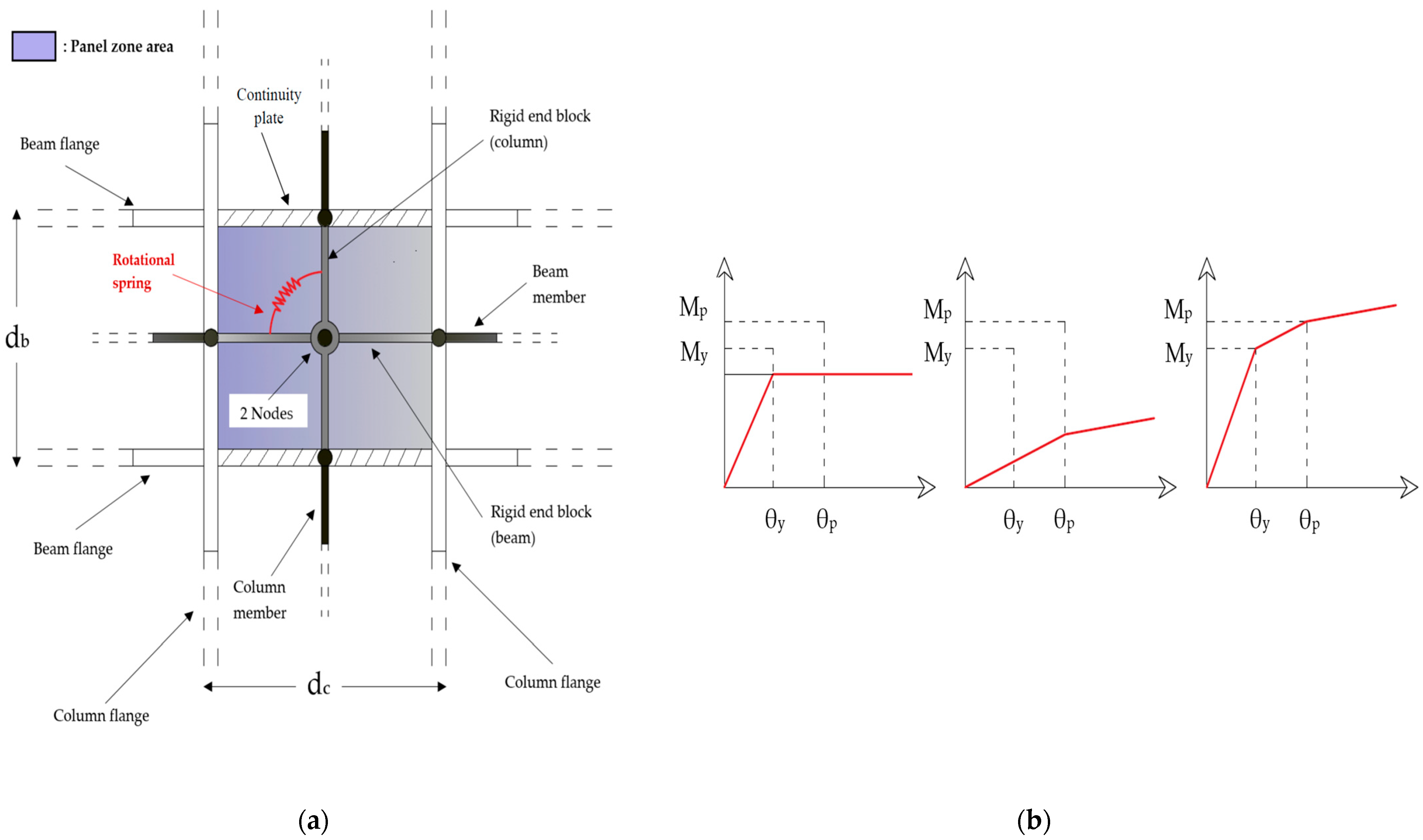
2.3. Frame Modeling and Nonlinear Time History Analyses

The seismic response of steel MRFs, with and without considering the panel zone effect, is investigated through extensive parametric analyses. These studies include nonlinear dynamic analyses of 15 frame configurations under 100 selected ground motions, utilizing the Ruaumoko2D (2006) software [28]. The analyses consider P–Δ effects by using the “large-displacement” analysis option. Furthermore, rigid diaphragm behavior is modeled at each floor to reflect the presence of a concrete slab. Beam members are modeled using the Giberson beam model [28], incorporating rotational springs (plastic hinges) at both ends without considering the interaction between moment capacity and axial force. Columns are represented by a steel beam-column model that accounts for the interaction between moment capacity and axial force [28]. In this study, the Giberson beam model with elastic hinges is employed. All members follow a bilinear hysteretic behavior, with a bilinear factor of 0.03 for both beams and columns. Strength and stiffness degradation phenomena have been incorporated as per reference [29]. For further details on the modeling of steel beams and columns, refer to [27]. The analyses employ Rayleigh damping with a damping ratio of ξ = 3% and utilize steel grade S275 as the structural material.

The panel zone plays a critical role in frame modeling and in the seismic behavior of steel MRFs. In this study, when its impact is examined, panel zone action has been incorporated at all column-beam intersections. The panel zone behavior is simulated using the “scissors model” [30], which effectively captures shear deformation through an equivalent zero-length rotational spring. Specifically, the model consists of two coincident nodes located at the intersection of the centroidal axes of a beam and a column (Figure 3a). Additionally, in Figure 3a, d_c denotes the height of the column cross-section and d_b denotes the height of the beam cross-section. The nonlinear behavior of the “scissors model” is represented by a trilinear moment-rotation (M, θ) relationship, as illustrated in Figure 3b. In Figure 3b, the first (from the left) diagram represents the moment-rotation behavior of the panel zone due to shear deformations, while the second (middle) diagram corresponds to the rotational response attributed to the rigid body motion of the adjoining members. The third (right) diagram is obtained by summing the contributions of the first two, providing the total moment-rotation (M-θ) response of the panel zone. The accuracy of this model has been validated through experimental comparisons and successfully applied in prior studies [4,31]. The “scissors model” was selected here for its simplicity and lower computational requirements, as opposed to more complex and computationally demanding models such as Krawinkler’s “parallelogram model” [1].

In this study, peak ground acceleration (PGA) is used as the intensity measure for nonlinear time history analyses (NTHAs) due to its widespread application. Using a straightforward bisection method, an iterative dynamic analysis procedure by means of Ruaumoko2D (2006) software [28] and Matlab [32] determines the scale factor that drives the structure to specific performance levels, defined by the interstorey drift ratio (IDR) and local ductility [21] (Table 6). Each scale factor corresponds to a particular frame, performance level, and seismic record. This scale factor is applied to the original accelerogram to achieve the desired damage level. To preserve the seismic characteristics of the ground motions, the maximum scale factor is constrained to 10, in accordance with [33]. Table 6 also presents the upper damage limits for steel MRFs at all performance levels. Additionally, NTHAs are conducted without scaling the accelerograms. Following each analysis, results such as base shear, interstory drift ratio (IDR), peak floor acceleration (PFA), and seismic reduction (behavior) factor (q) are extracted. Finally, these outcomes are compared for models with and without panel zone consideration to assess the panel zone’s influence on the seismic performance of the steel MRFs.

Table 6. Response limit values for the performance levels of plane steel MRFs (SEAOC, 2000) [21].

Performance Level	IDR	θp
SP1 or IO	0.7%	0
SP2 or DL	1.5%	θy
SP3 or LS	2.5%	3.5 θy
SP4 or CP	5.0%	6.5 θy

Table 6. Response limit values for the performance levels of plane steel MRFs (SEAOC, 2000) [21].

Performance Level	IDR	θp
SP1 or IO	0.7%	0
SP2 or DL	1.5%	θy
SP3 or LS	2.5%	3.5 θy
SP4 or CP	5.0%	6.5 θy

3. Computation of Seismic Behavior Factor q

The seismic reduction factor q, also known as the behavior factor, reduces the seismic forces used for design from the elastic force demands by accounting for the structure’s capacity to undergo inelastic deformation and its inherent overstrength. Many seismic codes like EC8 [22]) specify baseline q-values, but more refined approaches can yield deeper insights into how real structures transition from elasticity to inelastic behavior. Researchers such as Krawinkler and Seneviratna (1998) [34] and Fajfar (1999) [35] have discussed incremental dynamic analysis (IDA) or capacity-spectrum methods to quantify ductility. Meanwhile, Uang (1991) [36] emphasized that the seismic force reduction factor encompasses both ductility and overstrength, highlighting the extra margin between design expectations and true structural capacity.

In steel moment-resisting frames (MRFs), the panel zone can significantly affect the global inelastic response, as it often sustains shear deformations that alter how beam-column connections yield. For example, Castro et al. (2005) [2] showed that neglecting panel zone inelasticity may underpredict overall frame drift. Because the panel zone plays a key role in dissipating energy, its contribution to ductility translates into changes in the behavior factor and, hence, impacts the overall seismic behavior of steel MRFs.

Rather than equating behavior factor q to a ratio of elastic and yield base shears, this work employs scale factors (SF). Each ground motion is scaled until the first yield occurs at SF_y. The same motion is then scaled further up to SF_PL, at which a target performance level (see Table 6) is reached. Then, the behavior factor q is defined as follows:

$$q={\displaystyle \frac{{SF}_{PL}}{{SF}_y}}$$

(1)

Thus, capturing how much more seismic intensity the frame can accommodate beyond initial yielding. This approach preserves the original frequency content and duration of each earthquake, limiting the maximum scale factor to around 10 so as not to crucially distort the ground motion [33]. Because panel zone flexibility affects both SF_y and SF_PL, it inevitably influences the resulting q values. Consequently, the behavior factor reflects the overall seismic behavior of steel MRFs, including how panel zone deformation redistributes and absorbs energy during strong earthquake motions.

4. Analysis Results

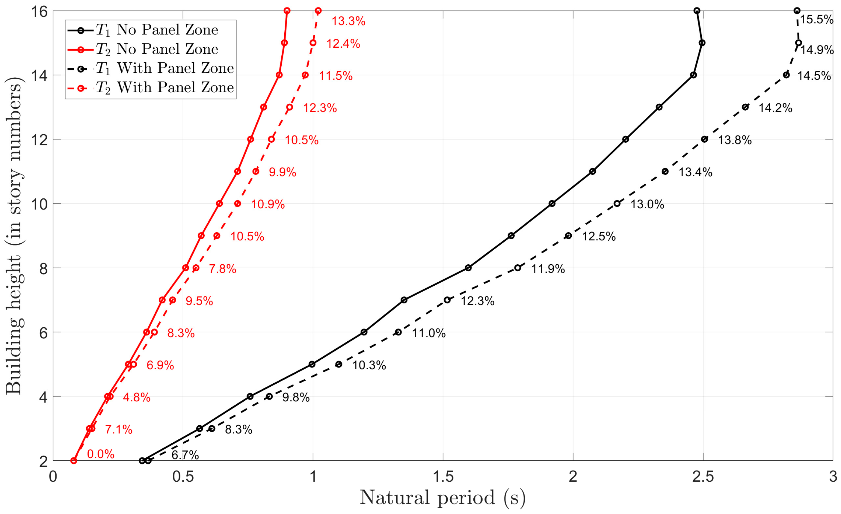
4.1. Influence of Panel Zone on the Modal Characteristics of Steel MRFs

Figure 4 illustrates the impact of incorporating panel zone flexibility on the fundamental (T₁) and second (T₂) vibration periods of the 15 steel MRFs as building height increases. The comparison between the cases of considering panel zone and without considering panel zone reveals that modeling panel zone consistently increases the periods for both vibration modes. These increases, highlighted as percentages alongside the “with panel zone curves” become especially significant for taller buildings, exceeding 15% in some cases. The findings emphasize the critical importance of considering panel zone flexibility in dynamic analyses, as it influences not only the fundamental mode of vibration but also the behavior of higher modes. The impact of the increased natural periods is explored in later sections, where seismic behavior factors, interstory drift ratios (IDRs), base shear, and other key response parameters are analyzed both with and without the consideration of the panel zone effect.

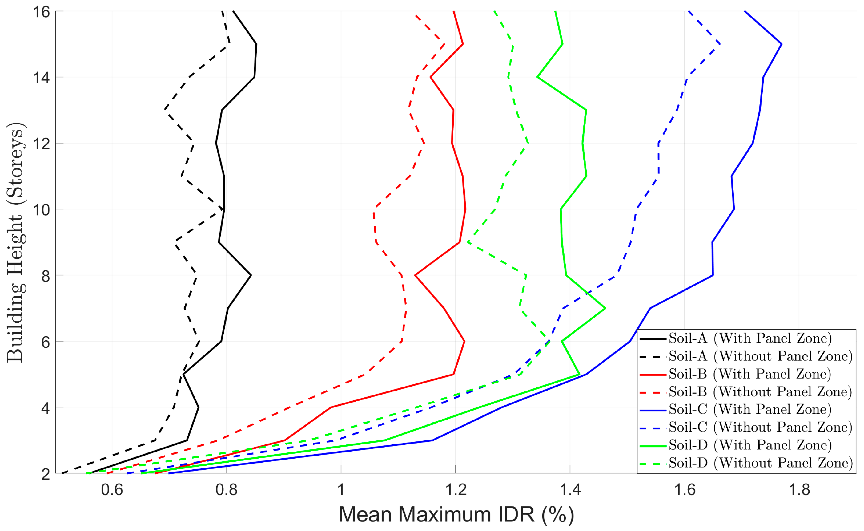
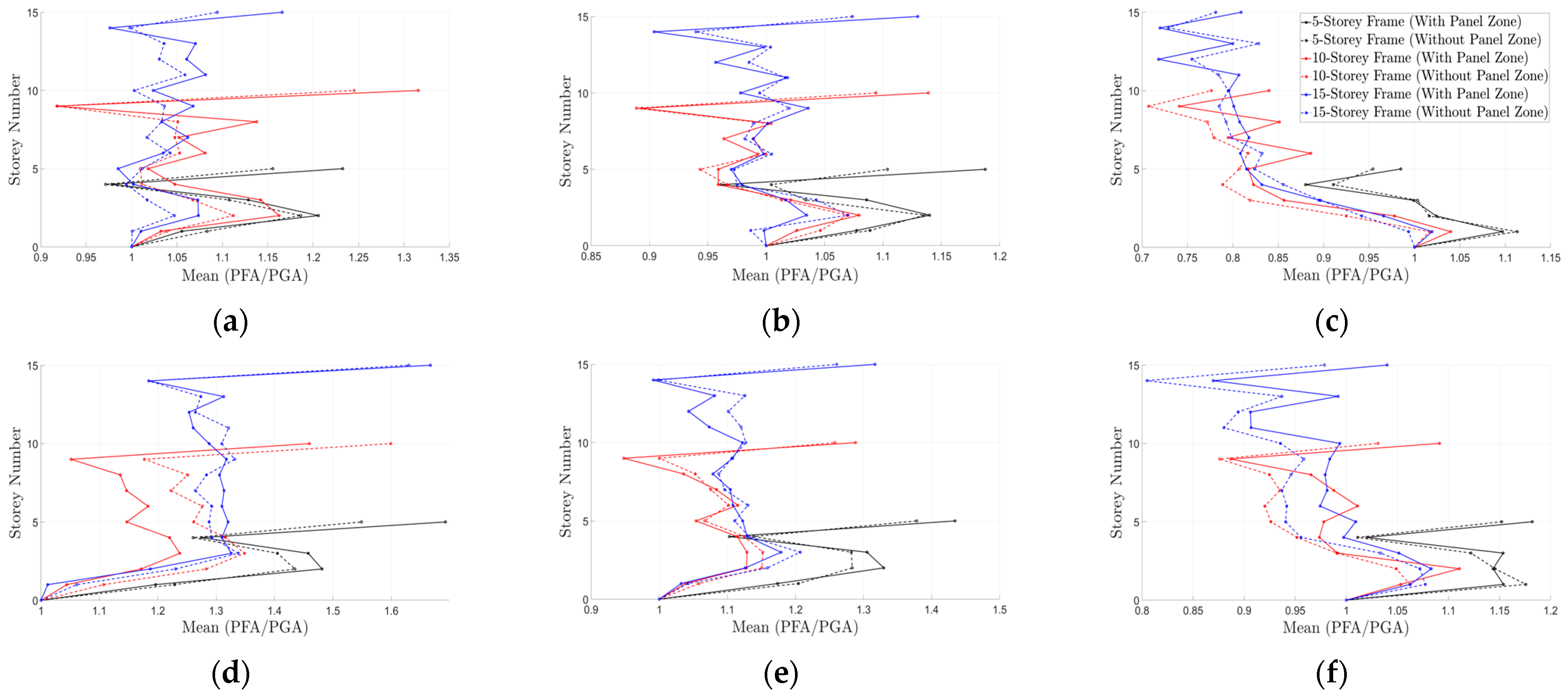
4.2. Influence of Panel Zone on the Seismic Behavior of Steel MRFs

Figure 5 illustrates the mean base shear developed in steel moment-resisting frames (MRFs) ranging from 2 to 16 storeys under earthquake records scaled to achieve various performance levels (DL, LS, and CP). The results are presented for soil types A, B, C, and D, as defined in EC8 [22]. As expected, higher target damage or performance levels correspond to higher mean base shears, reflecting the increased seismic demand necessary to drive the frames into more advanced inelastic states. Notably, neglecting the panel zone generally results in larger base shears, likely because including a panel zone reduces the global stiffness, allowing the same performance level to be reached without excessively scaling the ground motions. Consequently, overlooking panel zone effects leads to an overestimation of base shear demand and, therefore, a more conservative and potentially more expensive seismic design. The difference between frames modeled with and without panel zones becomes more pronounced as building height increases, indicating that the influence of panel zone stiffness is amplified in taller structures. Furthermore, subplots (a)–(d) show that stiffer soils (types A or B) generally result in higher base shear compared to softer soils (types C or D) for frames up to approximately 12 storeys under the same performance levels.

The variation in mean values of maximum IDRs across buildings of different heights subjected to earthquakes compatible with four soil types (A through D) according to EC8 [22], comparing scenarios with and without panel zones in steel MRFs, is illustrated in Figure 6. Since the earthquake records used are unscaled, the IDRs presented are not tied to any specific damage or performance level (Table 6). Instead, they provide a relative comparison of structural response across different soil types and frame configurations with or without the consideration of panel zone. In general, the curves indicate that mean values of maximum IDR increase with building height, reflecting larger lateral displacements at upper storeys. For buildings up to approximately five storeys, soils C and D exhibit relatively similar IDR levels regardless of panel zone inclusion. However, beyond five storeys, a more evident divergence emerges, suggesting that panel zones and softer soils have a greater impact as building height increases. Frames with panel zones tend to exhibit slightly higher (or differently distributed) drifts compared to those without panel zones, highlighting the additional flexibility the panel zone brings to the connection region under seismic loads. The comparison across soil types reveals that softer soils, such as types C and D, generally result in higher drift demands, while stiffer soils, such as types A and B, produce comparatively smaller IDRs. The observed IDR range, from approximately 0.5% to 1.8%, aligns with expectations for mid- to high-rise frames subjected to these specific ground motions. A plausible explanation, illustrated by Figure 2, is that while the stiffer soil (type A) may exhibit a slightly higher peak ground acceleration (PGA) amplification at very short periods, its spectral amplification quickly diminishes beyond that short-period range. In contrast, the softer soils (B, C, and D) display a broader range of amplification, extending into the medium-to-long-period domain where taller frames typically resonate. Consequently, even though soil A might have a relatively higher spike at short periods, it does not significantly excite buildings with longer fundamental periods, leading to comparatively smaller interstorey drift ratios (IDRs) in mid- to high-rise frames. Meanwhile, the softer soils maintain higher spectral ordinates over a wider period range, imposing greater seismic demands on taller structures and, thereby, resulting in greater IDRs overall.

Knowing how the peak floor acceleration (PFA) compares to the peak ground acceleration (PGA) at each level of a building helps engineers identify where seismic waves are amplified as they travel upward. This amplification profile is crucial for designing and detailing nonstructural elements (e.g., equipment, ceilings, and cladding) that can experience accelerations significantly higher than at the base, thus guiding seismic restraints and enhancing safety. Miranda and Taghavi (2005) [37] highlighted that analyzing peak floor acceleration-to-peak ground acceleration (PFA/PGA) ratios can help identify the storeys most susceptible to inelastic behavior and potential damage. Such understanding can lead to more effective seismic design and retrofit strategies. Additionally, Kalapodis et al. [38] conducted a comprehensive investigation of PFA/PGA ratios across a large number of steel frame configurations and evaluated the accuracy of the formulations provided in EC8 [22] and ASCE 7–16 [39].

The amplification of peak ground acceleration (PGA) along the height of 5-, 10-, and 15-story steel frames is depicted in Figure 7. Specifically, it presents the mean values of the ratio between peak floor acceleration (PFA) and peak ground acceleration (PGA) for all storeys of these frames. The seismic motions used for these plots are compatible with either soil type B (subplots (a)–(c)) or soil type D (subplots (d)–(f)). These motions have been appropriately scaled to drive the steel MRFs to one between three performance levels: damage limitation (DL), as shown in subplots (a) and (d), life safety (LS), as shown in subplots (b) and (e), or collapse prevention (CP) as shown in subplots (c) and (f). The five-story frame (with a period of 0.996 s without considering the panel zone) often aligns closely with the peak of the mean seismic response spectrum, particularly for soil types B, C, and D (see Figure 2). This alignment results in higher PFA/PGA ratios due to resonance effects. In contrast, the 10-story (with a first natural period of 1.919 s without considering panel zone) and 15-story (with a first natural period of 2.496 s without considering panel zone) frames fall within the descending branch of the mean response spectrum curve, where acceleration demands generally decrease. As a result, while taller frames may experience larger displacements, their fundamental periods no longer coincide with the dominant high-acceleration range. Therefore, the amplification of acceleration is strongly influenced by how closely a structure’s fundamental period aligns with the peak region of the mean response spectra curve for a given ground motion set.

One may observe that the highest story in each frame generally experiences the largest amplification of peak floor acceleration relative to the ground. Including the panel zone in the modeling, however, reduces this amplification, likely because the added joint flexibility moderates the overall dynamic response. In a purely rigid-joint model (i.e., no panel zone consideration), the top floor tends to develop greater inertial forces, thus yielding higher accelerations. By contrast, with panel zones considered, part of the deformation demand is absorbed within the joint region, reducing peak accelerations.

For the collapse prevention (CP) performance level, the seismic records are scaled to notably high intensities, up to ten times [33], resulting in a PGA that may exceed the peak floor accelerations (PFA) measured in the frame. In this deep inelastic state, significant regions of the structure yield and dissipate energy, effectively limiting the PFA. As a result, many times the PFA/PGA ratio falls below unity, leading to a phenomenon referred to as “de-amplification”. Instead of amplifying ground acceleration at higher storeys, the inelastic behavior of the structure restricts the PFA, preventing it from reaching or exceeding the PGA.

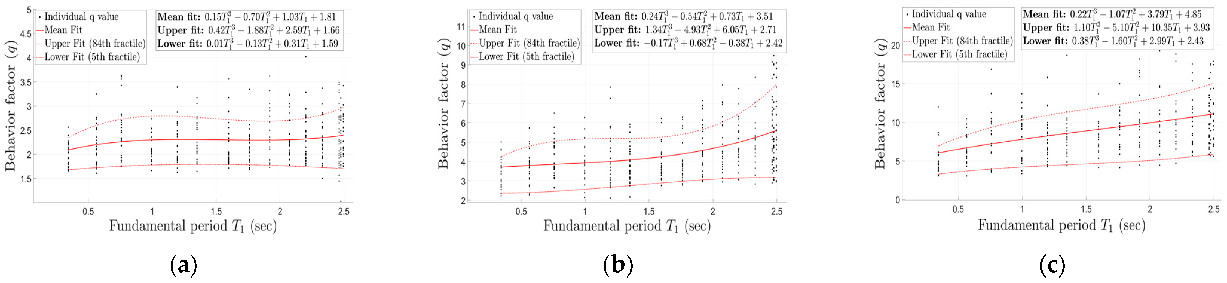
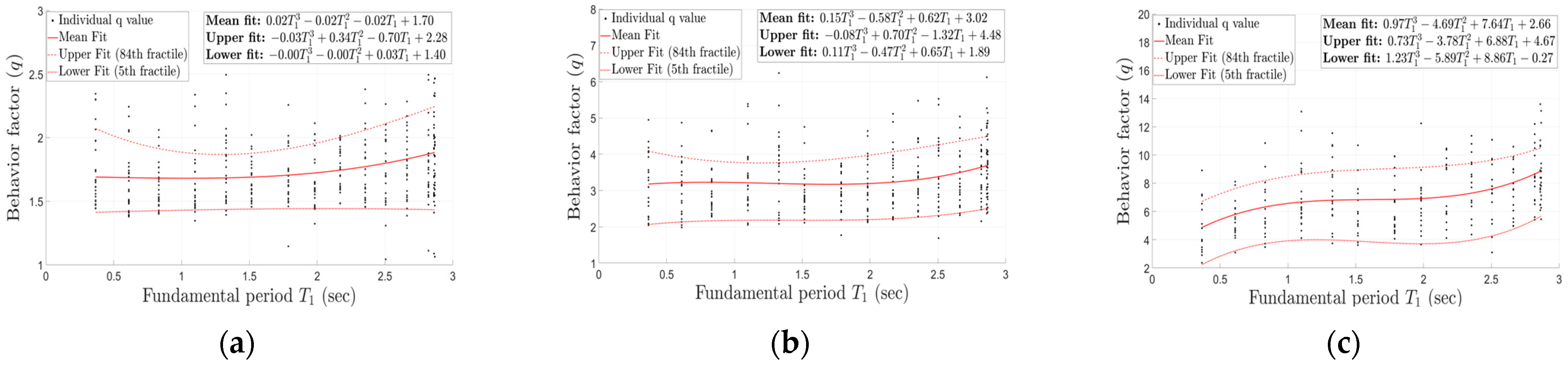
4.3. Influence of Panel Zone on the Behavior Factor

The impact of the panel zone on the seismic response of steel MRFs is mainly displayed through the behavior factor (termed as q by the EC8 [22]), which captures both ductility and overstrength. By comparing forces in an elastic model to those at a given performance level, q indicates how effectively the inelastic mechanisms reduce seismic demand. In this section, the equations defining q for each performance level, soil type, and with or without panel zone consideration are given in

Table 7. Proposed cubic polynomial equations for the behavior factor (q) corresponding to four soil types (A, B, C, and D) and three performance levels (DL, LS, and CP). Each soil type and performance level includes three bounding limits (upper, mean, and lower). Panel zone effects are not considered.

Performance Level	Limits	Soil Type—A	Soil Type—B	Soil Type—C	Soil Type—D
Damage limitation (DL) 0.7% < IDRmax ≤ 1.5%	Upper	${0.34T}_1^3-1.08T_1^2+0.66T_1+2.86$	${0.36T}_1^3-1.62T_1^2+2.15T_1+1.98$	${0.42T}_1^3-1.88T_1^2+2.59T_1+1.66$	${0.23T}_1^3-1.26T_1^2+2.22T_1+1.91$
	Mean	${0.23T}_1^3-0.81T_1^2+0.66T_1+2.25$	${0.26T}_1^3-1.20T_1^2+1.66T_1+1.65$	${0.15T}_1^3-0.70T_1^2+1.03T_1+1.81$	${0.20T}_1^3-1.02T_1^2+1.67T_1+1.59$
	Lower	${-0.01T}_1^3-0.29T_1^2+0.84T_1+2.21$	${0.02T}_1^3-0.10T_1^2+0.24T_1+1.59$	${0.01T}_1^3-0.13T_1^2+0.31T_1+1.59$	${0.15T}_1^3-0.70T_1^2+1.01T_1+1.34$
Life safety (LS) 1.5% < IDRmax ≤ 2.5%	Upper	${0.50T}_1^3-0.67T_1^2-1.51T_1+6.79$	${0.34T}_1^3-1.08T_1^2+1.13T_1+4.97$	${1.34T}_1^3-4.93T_1^2+6.05T_1+2.71$	${1.54T}_1^3-7.15T_1^2+10.60T_1+0.97$
	Mean	${0.63T}_1^3-2.03T_1^2+1.62T_1+3.87$	${0.73T}_1^3-3.14T_1^2+4.34T_1+2.42$	${0.24T}_1^3-0.54T_1^2+0.73T_1+3.51$	${1.42T}_1^3-6.35T_1^2+8.92T_1+0.68$
	Lower	${-0.39T}_1^3+1.64T_1^2-1.86T_1+2.87$	${0.65T}_1^3-2.80T_1^2+3.76T_1+1.35$	${-0.17T}_1^3+0.68T_1^2-0.38T_1+2.42$	${0.44T}_1^3-2.16T_1^2+3.34T_1+1.22$
Collapse prevention (CP) 2.5% < IDRmax ≤ 5%	Upper	${2.80T}_1^3-8.80T_1^2+7.77T_1+9.17$	${2.79T}_1^3-11.53T_1^2+16.07T_1+4.23$	${1.10T}_1^3-5.10T_1^2+10.35T_1+3.93$	${4.75T}_1^3-20.35T_1^2+29.43T_1+1.98$
	Mean	${1.26T}_1^3-4.01T_1^2+3.85T_1+6.56$	${2.20T}_1^3-9.40T_1^2+13.94T_1+1.82$	${0.22T}_1^3-1.07T_1^2+3.79T_1+4.85$	${3.80T}_1^3-16.35T_1^2+23.34T_1-1.82$
	Lower	${-0.32T}_1^3+0.54T_1^2+1.07T_1+2.82$	${0.48T}_1^3-2.90T_1^2+6.63T_1+1.92$	${0.38T}_1^3-1.60T_1^2+2.99T_1+2.43$	${0.81T}_1^3-4.22T_1^2+6.87T_1+0.59$

and

Table 8. Proposed cubic polynomial equations for the behavior factor (q) corresponding to four soil types (A, B, C, and D) and three performance levels (DL, LS, and CP). Each soil type and performance level includes three bounding limits (upper, mean, and lower). Panel zone effects are considered.

Performance Level	Limits	Soil Type—A	Soil Type—B	Soil Type—C	Soil Type—D
Damage limitation (DL)0.7% < IDRmax ≤ 1.5%	Upper	${0.01T}_1^3+0.10T_1^2-0.32T_1+2.05$	${-0.03T}_1^3+0.34T_1^2-0.70T_1+2.28$	${0.11T}_1^3-0.53T_1^2+0.85T_1+1.55$	${-0.02T}_1^3-0.04T_1^2+0.53T_1+1.54$
	Mean	${0.06T}_1^3-0.18T_1^2+0.14T_1+1.64$	${0.02T}_1^3-0.02T_1^2-0.02T_1+1.70$	${0.01T}_1^3-0.04T_1^2+0.15T_1+1.56$	${0.03T}_1^3-0.22T_1^2+0.56T_1+1.38$
	Lower	${-0.08T}_1^3+0.40T_1^2-0.49T_1+1.46$	${-0.00T}_1^3-0.00T_1^2+0.03T_1+1.40$	${-0.03T}_1^3+0.16T_1^2-0.21T_1+1.48$	${0.03T}_1^3-0.19T_1^2+0.34T_1+1.26$
Life safety (LS)1.5% < IDRmax ≤ 2.5%	Upper	${-0.04T}_1^3+1.69T_1^2-5.08T_1+7.19$	${-0.08T}_1^3+0.70T_1^2-1.32T_1+4.48$	${0.45T}_1^3-1.83T_1^2+2.40T_1+2.80$	${0.10T}_1^3-0.56T_1^2+1.39T_1+3.08$
	Mean	${0.37T}_1^3-1.18T_1^2+0.69T_1+3.20$	${0.15T}_1^3-0.58T_1^2+0.62T_1+3.02$	${0.13T}_1^3-0.40T_1^2+0.55T_1+2.76$	${0.24T}_1^3-1.12T_1^2+1.83T_1+2.31$
	Lower	${-0.06T}_1^3+0.29T_1^2-0.41T_1+2.25$	${0.11T}_1^3-0.47T_1^2+0.65T_1+1.89$	${-0.03T}_1^3+0.10T_1^2-0.08T_1+2.02$	${0.31T}_1^3-1.46T_1^2+2.17T_1+1.19$
Collapse prevention (CP)2.5% < IDRmax ≤ 5%	Upper	$-{0.30T}_1^3+4.15T_1^2-8.80T_1+12.59$	${0.73T}_1^3-3.78T_1^2+6.88T_1+4.67$	${1.45T}_1^3-6.60T_1^2+10.27T_1+3.23$	${2.05T}_1^3-10.28T_1^2+16.64T_1+1.15$
	Mean	${0.36T}_1^3-0.82T_1^2+0.50T_1+5.98$	${0.97T}_1^3-4.69T_1^2+7.64T_1+2.66$	${0.60T}_1^3-2.92T_1^2+5.36T_1+3.15$	${1.48T}_1^3-7.24T_1^2+11.47T_1+1.14$
	Lower	${0.34T}_1^3-2.12T_1^2+4.02T_1+1.60$	${1.23T}_1^3-5.89T_1^2+8.86T_1-0.27$	${-0.03T}_1^3-0.02T_1^2+1.23T_1+2.25$	${1.23T}_1^3-5.97T_1^2+8.68T_1-0.07$

. Furthermore, examples of q-factor curves are shown in Figure 8, Figure 9, Figure 10, Figure 11 and Figure 12.

As shown in Figure 12, higher performance levels correspond to higher values of q factors, reflecting the increased inelasticity demand and energy dissipation required to reach these levels. The inclusion of the panel zone reduces q values across all soil types due to its influence on global stiffness and the redistribution of inelastic deformations. This reduction is more evident for higher performance levels and softer soils (e.g., C and D). Although incorporating the panel zone can increase a frame’s overall ductility by allowing more inelastic deformation at the connections, it also lowers the global stiffness of the system. As a result, the seismic motions do not have to be scaled as extensively to reach a given performance or damage level, defined in terms of interstorey drift ratio (IDR). Meanwhile, the scale factor at first yield (SFy) remains almost the same either considering or not the panel zone action, because the onset of initial yielding is not drastically affected by joint flexibility. Hence, when computing the behavior factor q as the ratio of the scale factor at the performance level (SP_PL) to SFy, the panel zone case yields a lower SP_PL (due to reduced stiffness and earlier attainment of the target IDR). Consequently, $q={\displaystyle \frac{{SF}_{PL}}{{SF}_y}}$ is smaller, even though the frame could, in theory, accommodate greater ductility under higher excitations. The key point is that the target damage is a threshold that is reached at a lower scale factor once the panel zone’s flexibility is taken into account, thereby reducing the ratio of scale factors that define the q factor.

5. Discussion

The scissors model is chosen for its computational efficiency, making it suitable for large-scale parametric studies. However, it lumps panel zone shear deformations into a single rotational spring, which limits its ability to capture local stress distributions and web-flange interactions. In contrast, more complex models like Krawinkler’s parallelogram model provide a more detailed representation of joint shear deformation but require higher computational effort and detailed material data. Studies have shown that while both models give similar results in elastic analysis, differences arise under high ductility demands, with the parallelogram model offering greater accuracy [40]. Despite these limitations, the scissors model remains a practical choice for assessing global seismic response due to its balance between efficiency and reasonable accuracy.

In analyzing the effect of the panel zone on seismic design parameters, it may initially appear contradictory that including a more flexible joint region, often associated with higher ductility, can result in lower seismic behavior factors q. However, this outcome lies in how the added flexibility alters the scaling needed to achieve specific performance thresholds, ultimately influencing the computed q factor. The reduction in q factors due to the consideration of the panel zone action at certain performance levels can be explained by its impact on global stiffness and deformation distribution. When the panel zone is considered, the global stiffness of the frame decreases, resulting in reduced resistance to lateral forces. This lower stiffness means that achieving a specific damage or performance level, defined by a target interstorey drift ratio (IDR) or local ductility (Table 6), requires less scaling of the seismic motions. Thus, while the panel zone allows for higher global deformation capacity and improves the frame’s overall ductility, the scale factor required to reach a specific performance level (SF_PL) is reduced because the structure deforms more easily. Specifically, it is observed that the scale factor required to reach the first yield state (SF_y) is almost equal for frames with and without the consideration of panel zones. Since the q factor, in this study, is computed as the ratio of the scaling factors ($q={\displaystyle \frac{{SF}_{PL}}{{SF}_y}}$), and SF_y remains nearly constant; the reduction in q is governed by the lower SF_PL values are lower for frames that include panel zones. In other words, panel zones help achieve the desired performance levels at lower seismic intensities because they reduce frame stiffness and help spread the inelastic deformation more evenly across structural members. As a result, the frame requires less seismic energy to reach a specific drift level or damage state.

Neglecting the panel zone assumes the joint area is completely rigid, making the frame stiffer and reducing its ability to absorb energy within the panel zone area. As a result, seismic forces are estimated to be higher, which can lead to an overestimation of the base shear. While this creates a conservative safety margin, reducing the risk of under-designed frames, it also requires larger structural members and stronger detailing, increasing construction costs. Consequently, this study shows that ignoring the flexibility of the panel zone enhances safety but reduces cost efficiency, as it does not account for the actual inelastic deformation capacity of the frame.

These findings highlight the need for explicit guidance in EC8 regarding panel zone modeling. Specifically, recognizing the impact of the panel zone on global stiffness and inelastic behavior could lead to a more refined definition of the behavior factor q. Adjusting q or incorporating clear modeling provisions for panel zone flexibility would contribute to more cost-effective designs while maintaining structural safety.

6. Conclusions

This study examines the impact of panel zone modeling on the seismic response of steel moment-resisting frames (MRFs), taking into account different building heights (from 2 to 16 storeys) and soil types (A, B, C, or D according to the categorization of EC8). The key findings are summarized as follows:

• Including the panel zone in the analytical model reduces overall frame stiffness, thereby increasing the fundamental periods. For 16-story (and taller) buildings, the first-mode period increases by more than 15% and the second-mode period by over 13%, relative to models that neglect panel-zone action.
• Omitting the modeling of the panel zone leads to higher stiffness estimates and, therefore, larger base shear values during seismic analysis. Although this results in a more conservative design, improving safety margins, it also raises construction costs.
• As building height increases, the difference in base shear between two similar steel MRFs with and without panel zone consideration becomes more evident.
• Softer soils (e.g., type C or D) amplify ground motions over a broader period range, increasing mean maximum IDR values. The consideration of panel zone flexibility further raises drift response, especially in taller frames.
• The panel zone action contributes to the frame’s inelastic deformation, reduces stiffness, and decreases PGA amplification, especially at higher levels. Ignoring the panel zone influence results in an artificially stiff model, leading to increased floor accelerations.
• Because the panel zone lowers global stiffness, less seismic intensity is needed to reach a given damage level, reducing ${\displaystyle \frac{{SF}_{PL} }{{SF}_y}}$ ratio and, hence, the corresponding behavior factor q.

Overall, these findings highlight the importance of accurately modeling the panel zone for a realistic assessment of the seismic performance of a structure. While excluding the panel zone increases safety margins through higher design forces (base shear), it can also lead to unnecessarily conservative and costly designs. Consequently, accounting for panel zone flexibility is recommended, especially for taller frames and softer soils, to capture the redistribution of inelastic demands more accurately and align the design with actual structural behavior.

Possible limitations of this study include the exclusive use of the scissors model to represent panel zone behavior. While this model is widely utilized, validating the parametric analyses with alternative panel zone modeling approaches (e.g., the parallelogram model) would enhance the reliability of the findings. Additionally, this study does not examine frame behavior, with or without panel zones, under near-collapse conditions. Investigating the influence of the panel zone on structural response under extreme seismic demands could provide further insights into failure mechanisms and overall structural stability. Another limitation is the focus on a single frame configuration, the MRF. Exploring frame configurations other than MRFs would help capture a broader range of design practices. Finally, extending the analyses to 3D steel MRFs would allow for the consideration of out-of-plane effects and further strengthen the applicability of the results.

References

1. Krawinkler, H. Shear in Beam-Column Joints in Seismic Design of Steel Frames. Eng. J. Am. Inst. Steel Constr. 1978, 15, 82–91. [Google Scholar] [CrossRef]
2. Castro, J.M.; Elghazouli, A.Y.; Izzuddin, B.A. Modelling of the Panel Zone in Steel and Composite Moment Frames. Eng. Struct. 2005, 27, 129–144. [Google Scholar] [CrossRef]
3. Castro, J.M.; Dávila-Arbona, F.J.; Elghazouli, A.Y. Seismic Design Approaches for Panel Zones in Steel Moment Frames. J. Earthq. Eng. 2008, 12 (Suppl. S1), 34–51. [Google Scholar] [CrossRef]
4. Schneider, S.P.; Amidi, A. Seismic Behavior of Steel Frames with Deformable Panel Zones. J. Struct. Eng. 1998, 124, 35–42. [Google Scholar] [CrossRef]
5. Miri, M.; Naghipour, M.; Kashiryfar, A. Panel Zone Rigidity Effects on Special Steel Moment-Resisting Frames According to the Performance Based Design. World Acad. Sci. Eng. Technol. 2009, 50, 925–931. [Google Scholar]
6. Sui, W.; Dong, Z.; Zhang, X.; Wang, Z. Experimental Study of the Influence of the Shear Strength of Panel Zones on the Mechanical Properties of Steel Frame Structures. Structures 2022, 44, 42–57. [Google Scholar] [CrossRef]
7. Garlock, M.M.; Ricles, J.M.; Sause, R. Influence of Design Parameters on Seismic Response of Post-Tensioned Steel MRF Systems. Eng. Struct. 2008, 30, 1037–1047. [Google Scholar] [CrossRef]
8. Herrera, R.A.; Muhummud, T.; Ricles, J.M.; Sause, R. Modeling of Composite MRFs with CFT Columns and WF Beams. Steel Compos. Struct. 2022, 43, 327–340. [Google Scholar] [CrossRef]
9. Herrera, R.; Nunez, E.; Hernandez, M. Seismic-Resistant Performance of Double Built-Up T Moment Connections. J. Struct. Eng. 2025, 151, 04024193. [Google Scholar] [CrossRef]
10. Du, H.; Zhao, P.; Wang, Y.; Sun, W. Seismic Experimental Assessment of Beam-Through Beam-Column Connections for Modular Prefabricated Steel Moment Frames. J. Constr. Steel Res. 2022, 192, 107208. [Google Scholar] [CrossRef]
11. Mansouri, I.; Saffari, H. A New Steel Panel Zone Model Including Axial Force for Thin to Thick Column Flanges. Steel Compos. Struct. 2014, 16, 417–436. [Google Scholar] [CrossRef]
12. Sazmand, E.; Aghakouchak, A.A. Modeling the Panel Zone in Steel MR Frames Composed of Built-Up Columns. J. Constr. Steel Res. 2012, 77, 54–68. [Google Scholar] [CrossRef]
13. Xu, Z.-G.; Zhao, Y.-T.; Wu, H.-J.; Bao, E.-H. Research on the Influence of Panel Zone on Dynamic Damage of Multi-Story Steel Structure. Eur. J. Environ. Civ. Eng. 2024, 28, 518–533. [Google Scholar] [CrossRef]
14. Skiadopoulos, A.; Lignos, D.G. Seismic Demands of Steel Moment-Resisting Frames with Inelastic Beam-to-Column Web Panel Zones. Earthq. Eng. Struct. Dyn. 2022, 51, 1591–1609. [Google Scholar] [CrossRef]
15. Skiadopoulos, A.; Elkady, A.; Lignos, D.G. Proposed Panel Zone Model for Seismic Design of Steel Moment-Resisting Frames. J. Struct. Eng. 2021, 147, 04021006. [Google Scholar] [CrossRef]
16. Isaincu, A.; D’Aniello, M.; Stratan, A. Implications of Structural Model on the Design of Steel Moment Resisting Frames. Open Constr. Build. Technol. J. 2018, 12 (Suppl. S1), 124–131. [Google Scholar] [CrossRef]
17. Rigi, A.; JavidSharifi, B.; Hadianfard, M.A.; Yang, T.Y. Study of the Seismic Behavior of Rigid and Semi-Rigid Steel Moment-Resisting Frames. J. Constr. Steel Res. 2021, 186, 106910. [Google Scholar] [CrossRef]
18. Sepasdar, R.; Banan, M.R.; Banan, M.R. A Numerical Investigation on the Effect of Panel Zones on Cyclic Lateral Capacity of Steel Moment Frames. Iran. J. Sci. Technol. Trans. Civ. Eng. 2020, 44, 439–448. [Google Scholar] [CrossRef]
19. Lu, L.; Zhang, J.; Zhang, G.; Peng, H.; Liu, B.; Hao, H. The Influence of Box-Strengthened Panel Zone on Steel Frame Seismic Performance. Buildings 2023, 13, 3042. [Google Scholar] [CrossRef]
20. Tuna, M.; Topkaya, C. Panel Zone Deformation Demands in Steel Moment Resisting Frames. J. Constr. Steel Res. 2015, 110, 65–75. [Google Scholar] [CrossRef]
21. SEAOC. Recommended Lateral Force Requirements and Commentary; Structural Engineers Association of California: Sacramento, CA, USA, 1999. [Google Scholar]
22. EN 1998-1; Eurocode 8. Design of Structures for Earthquake Resistance, Part 1: General Rules, Seismic Actions and Rules for Buildings. European Committee for Standardization (CEN): Brussels, Belgium, 2009.
23. EN 1993-1-1; Eurocode 3. Design of Steel Structures—Part 1-1: General Rules and Rules for Buildings. European Committee for Standardization (CEN): Brussels, Belgium, 2005.
24. SAP2000 (Version 19); Analysis Reference Manual. Computers and Structures Inc.: Berkeley, CA, USA, 2019.
25. PEER. Pacific Earthquake Engineering Research Center, Strong Ground Motion Database; University of California: Berkeley, CA, USA, 2009; Available online: http://peer.berkeley.edu/ (accessed on 1 January 2015).
26. COSMOS. Consortium of Organizations for Strong Motion Observation Systems; COSMOS: San Francisco, CA, USA, 2013; Available online: http://www.cosmos-eq.org/ (accessed on 1 January 2015).
27. Kalapodis, N.A.; Papagiannopoulos, G.A.; Beskos, D.E. Modal Strength Reduction Factors for Seismic Design of Plane Steel Braced Frames. J. Constr. Steel Res. 2018, 147, 549–563. [Google Scholar] [CrossRef]
28. Carr, A.J. Theory and User Guide to Associated Programs—Ruaumoko Manual; Department of Engineering, University of Canterbury: Christchurch, New Zealand, 2006. [Google Scholar]
29. Lignos, D.G.; Krawinkler, H. Deterioration Modeling of Steel Components in Support of Collapse Prediction of Steel Moment Frames Under Earthquake Loading. J. Struct. Eng. 2011, 137, 1291–1302. [Google Scholar] [CrossRef]
30. FEMA 356. Prestandard and Commentary for the Seismic Rehabilitation of Buildings; Federal Emergency Management Agency: Washington, DC, USA, 2000. [Google Scholar]
31. Lee, C.H.; Jeon, S.W.; Kim, J.H.; Uong, C.M. Effects of Panel Zone Strength and Beam-Web Connection Method on Seismic Performance of Reduced Beam Section Steel Moment Connections. J. Struct. Eng. 2005, 131, 1854–1865. [Google Scholar] [CrossRef]
32. MATLAB, version 2018a; The MathWorks, Inc.: Natick, MA, USA, 2018.
33. De Luca, F.; Iervolino, I.; Cosenza, E. Unscaled, Scaled, Adjusted and Artificial Spectral Matching Accelerograms: Displacement and Energy-Based Assessment. In Proceedings of the 13th Congress of the Italian National Association of Earthquake Engineering (ANIDIS), Bologna, Italy, 28 June–2 July 2009. [Google Scholar]
34. Krawinkler, H.; Seneviratna, G.D.P.K. Pros and Cons of a Pushover Analysis of Seismic Performance Evaluation. Eng. Struct. 1998, 20, 452–464. [Google Scholar] [CrossRef]
35. Fajfar, P. Capacity Spectrum Method Based on Inelastic Demand Diagrams. Earthq. Eng. Struct. Dyn. 1999, 28, 979–993. [Google Scholar] [CrossRef]
36. Uang, C.M. Establishing R (or Rw) and Cd Factors for Building Seismic Provisions. J. Struct. Eng. 1991, 117, 19–28. [Google Scholar] [CrossRef]
37. Miranda, E.; Taghavi, S. Approximate Floor Acceleration Demands in Multistory Buildings. I: Formulation. J. Struct. Eng. 2005, 131, 203–211. [Google Scholar] [CrossRef]
38. Kalapodis, N.A.; Muho, E.V.; Papagiannopoulos, G.A. Integration of Peak Seismic Floor Velocities and Accelerations into the Performance-Based Design of Steel Structures. Soil Dyn. Earthq. Eng. 2022, 154, 107160. [Google Scholar] [CrossRef]
39. ASCE/SEI 7-16; Minimum Design Loads and Associated Criteria for Buildings and Other Structures. American Society of Civil Engineers: Reston, VA, USA, 2017.
40. Charney, F.A.; Marshall, J. A Comparison of the Krawinkler and Scissors Models for Including Beam–Column Joint Deformations in the Analysis of Moment-Resisting Steel Frames. Eng. J. (AISC) 2006, 43, 31–48. [Google Scholar] [CrossRef]
Figure 1. Plane steel MRFs of n storeys.
Applmech 06 00022 g001
Figure 2. Pseudo acceleration response spectra with the mean curve (blue dashed line), accounting for ξ = 5 % and (a) soil type A, or (b) soil type B, or (c) soil type C, or (d) soil type D.
Applmech 06 00022 g002
Figure 3. (a) Scissors model representation of the panel zone; (b) corresponding trilinear moment-rotation behavior used in Ruaumoko 2D [28].
Applmech 06 00022 g003
Figure 4. Variation of the natural periods (T1 and T2) of 15 steel MRFs with and without panel zone modeling as a function of building height. The percentages indicate the relative increase of natural periods due to the consideration of panel zones.
Applmech 06 00022 g004
Figure 5. Comparison of base shear versus building height for 15 steel MRFs subjected to earthquakes compatible with different soil types: (a) soil type A, (b) soil type B, (c) soil type C, and (d) soil type D. Each subplot presents curves corresponding to three performance levels (DL, LS, and CP), considering (continuous line) or neglecting (dashed line) the influence of panel zone.
Applmech 06 00022 g005
Figure 6. Comparison of mean values of maximum IDR versus building height for earthquakes corresponding to four soil types (A, B, C, and D) according to EC8, with and without the consideration of the panel zones.
Applmech 06 00022 g006
Figure 7. Mean PFA/PGA profiles for 5, 10, and 15-story steel MRFs, analyzed both with (solid lines) and without (dashed lines) the consideration of panel zones. Subplots (ac) correspond to ground motions compatible with soil type B, while subplots (df) correspond to ground motions compatible with soil type D. The ground motions have been properly scaled to force the frames to reach the DL (a,d), or LS (b,e), or CP (c,f) performance level. The x-axis represents the mean PFA/PGA, while the y-axis denotes the story number.
Applmech 06 00022 g007
Figure 8. Mean, upper, and lower fit curves of the q-factor corresponding to (a) DL, (b) LS, and (c) CP performance levels. Each data point in the scatter cloud is derived from nonlinear time history analyses using seismic recordings compatible with soil type B, as defined in EC8 [22]. Panel zone effects are not considered in the frame modeling.
Applmech 06 00022 g008
Figure 9. Mean, upper, and lower fit curves of the q-factor corresponding to (a) DL, (b) LS, and (c) CP performance levels. Each data point in the scatter cloud is derived from nonlinear time history analyses using seismic recordings compatible with soil type C, as defined in EC8 [22]. Panel zone effects are not considered in the frame modeling.
Applmech 06 00022 g009
Figure 10. Mean, upper, and lower fit curves of the q-factor corresponding to (a) DL, (b) LS, and (c) CP performance levels. Each data point in the scatter cloud is derived from nonlinear time history analyses using seismic recordings compatible with soil type B, as defined in EC8 [22]. Panel zone effects are considered in the frame modeling.
Applmech 06 00022 g010
Figure 11. Mean, upper, and lower fit curves of the q-factor corresponding to (a) DL, (b) LS, and (c) CP performance levels. Each data point in the scatter cloud is derived from nonlinear time history analyses using seismic recordings compatible with soil type C, as defined in EC8 [22]. Panel zone effects are considered in the frame modeling.
Applmech 06 00022 g011
Figure 12. Mean q value curves for the steel MRFs with and without the consideration of panel zone for three performance levels and for (a) soil type A, (b) soil type B, (c) soil type C, and (d) soil type D.
Applmech 06 00022 g012