Article

Measuring Residual Stresses with Crack Compliance Methods: An Ill-Posed Inverse Problem with a Closed-Form Kernel

DICI—Dipartimento di Ingegneria Civile e Industriale, Università di Pisa, 56122 Pisa, Italy
*
Author to whom correspondence should be addressed.
Appl. Mech. 2024, 5(3), 475-489; https://doi.org/10.3390/applmech5030027
Submission received: 1 June 2024 / Revised: 5 July 2024 / Accepted: 10 July 2024 / Published: 14 July 2024

Abstract

:
By means of relaxation methods, residual stresses can be obtained by introducing a progressive cut or a hole in a specimen and by measuring and elaborating the strains or displacements that are consequently produced. If the cut can be considered a controlled crack-like defect, by leveraging Bueckner’s superposition principle, the relaxed strains can be modeled through a weighted integral of the residual stress relieved by the cut. To evaluate residual stresses, an integral equation must be solved. From a practical point of view, the solution is usually based on a discretization technique that transforms the integral equation into a linear system of algebraic equations, whose solutions can be easily obtained, at least from a computational point of view. However, the linear system is often significantly ill-conditioned. In this paper, it is shown that its ill-conditioning is actually a consequence of a much deeper property of the underlying integral equation, which is reflected also in the discretized setting. In fact, the original problem is ill-posed. The ill-posedness is anything but a mathematical sophistry; indeed, it profoundly affects the properties of the discretized system too. In particular, it induces the so-called bias–variance tradeoff, a property that affects many experimental procedures, in which the analyst is forced to introduce some bias in order to obtain a solution that is not overwhelmed by measurement noise. In turn, unless it is backed up by sound and reasonable physical assumptions on some properties of the solution, the introduced bias is potentially infinite and impairs every uncertainty quantification technique. To support these topics, an illustrative numerical example using the crack compliance (also known as slitting) method is presented. The availability of the Linear Elastic Fracture Mechanics Weight Function for the problem allows for a completely analytical formulation of the original integral equation by which bias due to the numerical approximation of the physical model is prevented.

1. Introduction

When measuring the stresses generated by external loads acting on a component, a technique to directly measure stresses is seldom available. Much more commonly, an indirect measurement is pursued, for instance by recording the deformation fields produced by the application of the external loads with respect to a configuration where it is (sometimes implicitly) assumed that they are absent [1]. For example, strain gauges measure deformations that are referenced to the moment they were glued; also, non-contact techniques such as Digital Image Correlation (DIC) [2,3,4,5,6] or Electronic Speckle Pattern Interferometry (ESPI) [7,8,9] measure changes in the displacement fields by comparing an initial and a final state. Constitutive models of the material—usually elastic—are then used to reconstruct the stresses. In the case of residual stresses, which act in the absence of external loads and primarily arise to restore the compatibility of the displacement fields that develop during the production process, the critical missing element is precisely an unstressed reference state, and this absence is arguably the fundamental difficulty in measuring residual stresses [10].
Diffraction methods [11] address this issue by measuring the absolute spacing of the crystal lattice planes and comparing it with a reference unstressed value, obtained for that specific material using appropriate techniques. This process yields the deformation produced by the stresses, which then allows for their calculation using suitable constitutive models. On the other hand, relaxation methods physically recreate an unstressed state by removing or disconnecting a portion of the component’s domain [12,13,14,15,16,17,18,19]. This action sets certain stress components to zero, causing measurable deformations that can be correlated with the previously acting residual stress values. In other words, the process typically used for stresses produced by external loads is metaphorically followed in reverse, measuring the deformation produced by the removal of the stresses to be measured.
For technological reasons, it is often impossible to access the entire deformation field, which would allow for the pointwise determination of the complete stress fields. Instead, only measurements of certain deformation components within a subdomain of the analyzed specimen as the cut or removal process progresses are available. When using strain gauges, each grid provides an approximately pointwise measurement of a single deformation component. In the case of full-field techniques, the deformation measured is, at best, that of the external surfaces of the component, with a limited spatial resolution that depends on the specific measurement instrument.
Thanks to Bueckner’s superposition principle [20], it is still possible to reconstruct the stresses by proceeding as follows. It is assumed that the residual stresses to be measured belong to the span of an appropriate functional basis [21] (often piecewise constant functions or polynomials). Then, the linearity of the elastic problem is leveraged to generate the deformation histories that correspond to the chosen stress basis. Finally, this linear relationship is inverted to obtain the required stresses from the measured deformations.
In the general case, the fact that deformations produced by relaxation methods can be computed by summing the individual contributions from each point-wise value of the stress field is represented by an integral equation, whose typical form is the following:
ε h = 0 h A ( h , z ) σ ( z ) d z
where h characterizes the geometrical properties of the domain disconnection (such as the length of a cut), while z acts as a spatial coordinate in the specimen. In fact, Equation (1) states that, for a given cut length h, the deformations produced are a weighted sum—with weights denoted as A ( h , z ) —of the residual stresses that have been relaxed by the cut, as the component compliance depends point by point on the location where the stresses are removed [17,22,23,24]. A ( h , z ) is usually called the influence function, calibration function, or kernel of the problem; in a discrete setting, it becomes what is commonly referred to as the calibration matrix of the problem. Clearly, the actual form of Equation (1) depends on the specific problem, although this mathematical structure is generally maintained.
As is well known in the literature on residual stresses, determining stresses from deformations through Equation (1) is a problem that significantly challenges the accuracy of the measurement instruments used, as the resulting calculation is often extremely sensitive to input errors [25]. Formally, one would say that the problem is very ill-conditioned.
The authors pointed out in [26,27] that the ill-conditioning of the problem is actually just a symptom of another distinct (and arguably more important) mathematical property called ill-posedness, which is notably known to afflict Equation (1) by the mathematical literature. Its main characteristic consists of a lack of continuity of the solution from the initial data, which, from a practical standpoint, results in solutions having potentially infinite errors obtained from measurement instruments with finite confidence intervals.
In the previous works by the authors [28,29,30,31], the discussion was focused on the hole-drilling method, where the equation coincides exactly with Equation (1). In this paper, it is shown that an important class of residual-stress-measurement techniques borrowed from fracture mechanics—falling under the name of crack compliance methods—suffers from the same effects, although the equation upon which they are based may appear to be slightly different from Equation (1). In this regard, the work aims to improve the understanding of the mathematical foundations on which the method is based.
The work is organized as follows:
  • In Section 2, crack compliance methods and their fundamental equations are introduced, drawing on some basic concepts of fracture mechanics and thus arriving at the equation of the problem concerning the reconstruction of residual stresses.
  • In Section 3, the obtained equations are used to run some numerical experiments that expose the peculiar features of ill-posedness.
  • In Section 4, the practical consequences for the analyst who must navigate ill-posedness in a residual stress measurement are discussed.

2. Theoretical Background

2.1. Crack Compliance Methods

One of the most intuitive ways to mechanically disconnect a portion of a component for a residual stress analysis is arguably to introduce a cut, which creates two new surfaces on which the traction vector is forced to be null. The corresponding residual-stress-measurement technique was originally called the crack compliance method [16], and only in subsequent years it became known as the slitting method [32]. If the problem’s linearity holds, Bueckner’s superposition principle [20] holds as well, so the deformation fields generated by the cut are equivalent to those generated by applying tractions of opposite signs to those originally acting on the created surfaces (Figure 1).
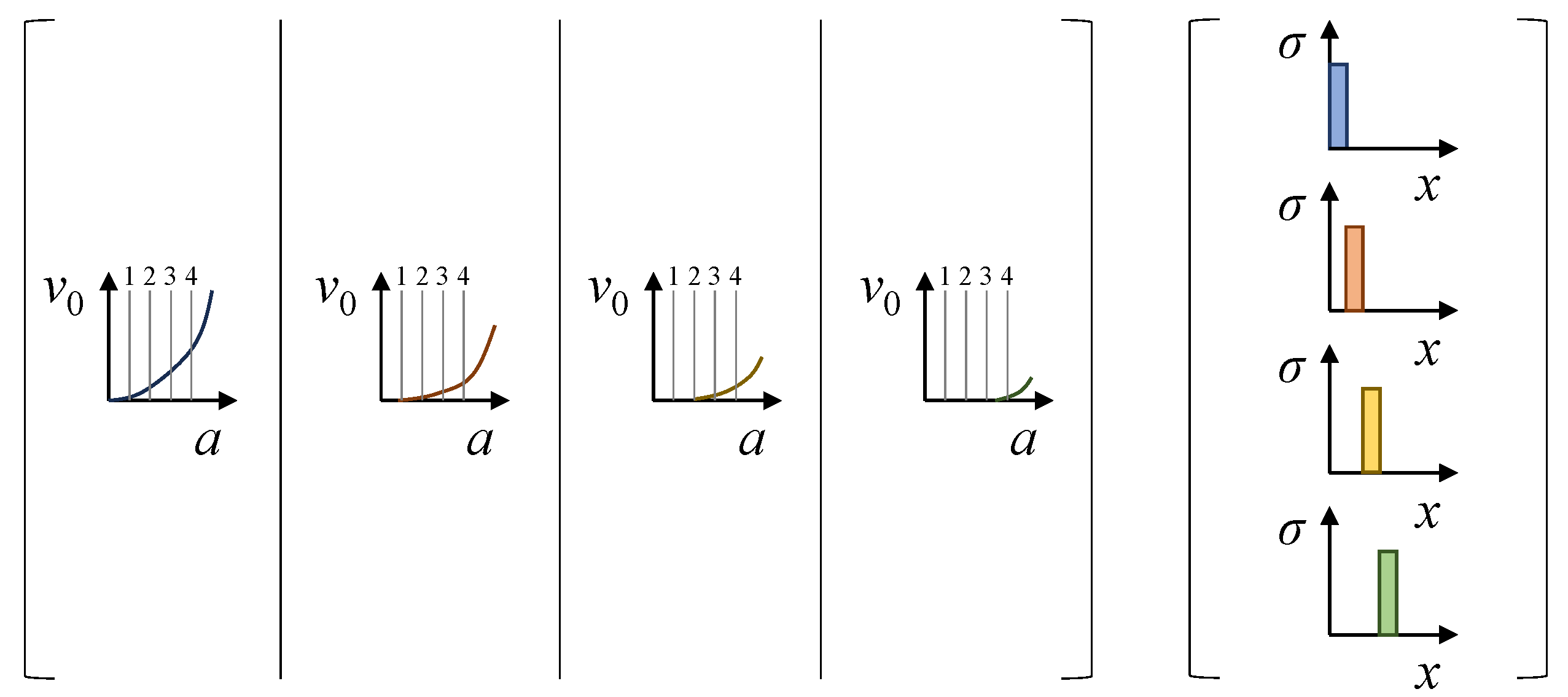
Thanks to the broad availability of finite element (FE) analyses, the state of the art for relaxation methods has evolved to directly generate the calibration matrix of the problem in discrete form through numerical simulations—as in Figure 2—even though this development may have sometimes led to overlooking the original mathematical nature of the problem. Given their great accuracy, strain gauges are usually placed on the front or back face to record strains at the specimen surface, instead of adopting displacement-measuring devices. Anyway, regardless on whether displacement or strain measurements are actually employed, a linear system is obtained. As explained in [26,27], what one obtains is simply a discrete realization of an integral equation like Equation (1), which then retains all its fundamental issues.
Before FE analyses became the standard for constructing calibration matrices, crack compliance methods had the huge advantage of allowing for the use of theoretical results from fracture mechanics to formulate the solving equations of the problem [33,34]. In fact, the solution fields corresponding to a plane crack in a semi-infinite or rectangular domain are among the most common results of fracture mechanics [35], which can be used to obtain an equation like Equation (1) without resorting to numerical computations.
For example, for a given crack face normal traction σ ( x ) , the stress intensity factor (SIF) for a 2D boundary value problem containing a crack of length a can be computed through the following equation [35]:
K I ( a ) = 0 a h ( a , x ) σ ( x ) d x
where h ( a , x ) is a weight function (WF) that can be shown to depend only on the geometry of the cracked body. As shown by Rice [36], if K I ( a ) and the crack face displacement v ( a , x ) —measured from the undeformed crack surface—are known for a given Mode I loading, then h ( a , x ) can effectively be computed as
h ( a , x ) = E K I ( a ) v ( a , x ) a
Recall that E depends on whether plane stress or plane strain conditions are assumed.
As h ( a , x ) is readily available—at worst, through a series expansion—for many 2D geometries, one can employ Equations (2) and (3) to write down the relation between the desired residual stresses and other measurable quantities. For example, as a longer crack is progressively introduced, one may measure the SIF through a technique of choice (such as the photoelastic method [33]) and correlate it with σ ( x ) through Equation (2), which has itself a very similar mathematical structure to Equation (1). As a matter of fact, they are both Volterra integral equations of the first kind [37].
Alternatively, one can measure the crack mouth opening displacement (CMOD) 2 v ( a , 0 ) and correlate it with the residual stresses by proceeding as follows. From Equation (3), one has
v ( a , 0 ) v 0 ( a ) = 1 E 0 a h ( s , 0 ) K I ( s ) d s
By substituting K I ( s ) from Equation (2) and rearranging:
v 0 ( a ) = 1 E 0 a h ( s , 0 ) 0 s h ( s , t ) σ ( t ) d t d s
v 0 ( a ) = 1 E 0 a 0 s h ( s , 0 ) h ( s , t ) σ ( t ) d t d s
Then, one can define
ψ ( a , x ) h ( a , 0 ) h ( a , x )
and write
v 0 ( a ) = 1 E 0 a 0 s ψ ( s , t ) σ ( t ) d t d s
which is another integral equation relating σ ( x ) and the measurable quantity v 0 ( a ) , albeit slightly more complex than Equation (2). The kernel function ψ ( a , x ) has units of 1 / Length and retains some properties of weight functions, including having an integrable singularity at x = a .
Equation (8) does not require FE analyses to identify residual stresses—as ψ ( a , x ) is usually available—and is of high practical significance, since crack opening displacement-measuring devices are widely available instruments in laboratories that perform fracture mechanics experiments. Despite the apparent differences with Equation (1) and its fully analytical formulation, the next section shows that this problem is still ill-posed.

2.2. Ill-Posedness

A peculiar characteristic of Equation (8) is that it acts as a low-pass filter with respect to oscillations of σ ( x ) along its domain. This is also intuitive from a physical perspective. The value of the CMOD is minimally affected by the short-scale variations in the stresses applied on the crack faces, as Saint Venant’s principle [38] ensures that boundary conditions with the same resultant actions on a given dimensional scale generate deformation fields whose differences are confined to a comparably sized region. Consequently, tractions with highly oscillatory behavior influence the CMOD primarily through their values averaged at longer dimensional scales, without locally self-equilibrated peaks affecting the result.
This intuitive statement has a formal mathematical explanation, too. The Riemann–Lebesgue lemma (see [39]) ensures that, if ψ ( a , x ) is integrable on its domain, then
lim N 0 a ψ ( a , t ) sin ( N t ) d t = 0 a 0 , a max
Similarly, by applying Lebesgue’s dominated convergence theorem [40], a further integration of a vanishing function can be shown to converge to zero as N , so that
lim N 0 a 0 s ψ ( s , t ) sin ( N t ) d t d s = lim N v N ( a , 0 ) a 0 , a max
This seemingly abstract mathematical feature has huge practical implications. For any positive real number k, by taking a sufficiently large N, we can generate a residual stress distribution σ δ ( x ) = k sin ( N x ) that has an arbitrarily low (yet non-null) effect v δ ( a , 0 ) on the measured CMOD. Due to the problem linearity, this implies that the measured samples can be perturbed by an arbitrarily low quantity v δ ( a , 0 ) and obtain another solution that differs from the true one by k sin ( N x ) , which, in turn, can be made arbitrarily high through the initial choice of k.
The resulting effect is an infinite sensitivity with respect to the input errors: through arbitrarily low measurement perturbations, the solution error cannot be bound by any inequality. A mathematical problem that shows this effect is referred to as an ill-posed problem. Yet, as explained in Section 3, the problem is seldom analytically solved in infinite-dimensional function spaces, as the usual solution procedure involves a discretization phase that is then followed by numerical computations.
By acquiring a finite number of measurement points and representing the solution with a finite number of coordinates, only a finite-dimensional approximation of the original problem is being solved. In this new problem, the sensitivity to error cannot be infinite—the dimensional scale of the oscillations allowed in the solution cannot decrease indefinitely—but it can be high enough to challenge the accuracy of the measurement instruments used. Then, the problem is said to be ill-conditioned, which in this case is only a consequence of the discretization of an ill-posed problem.
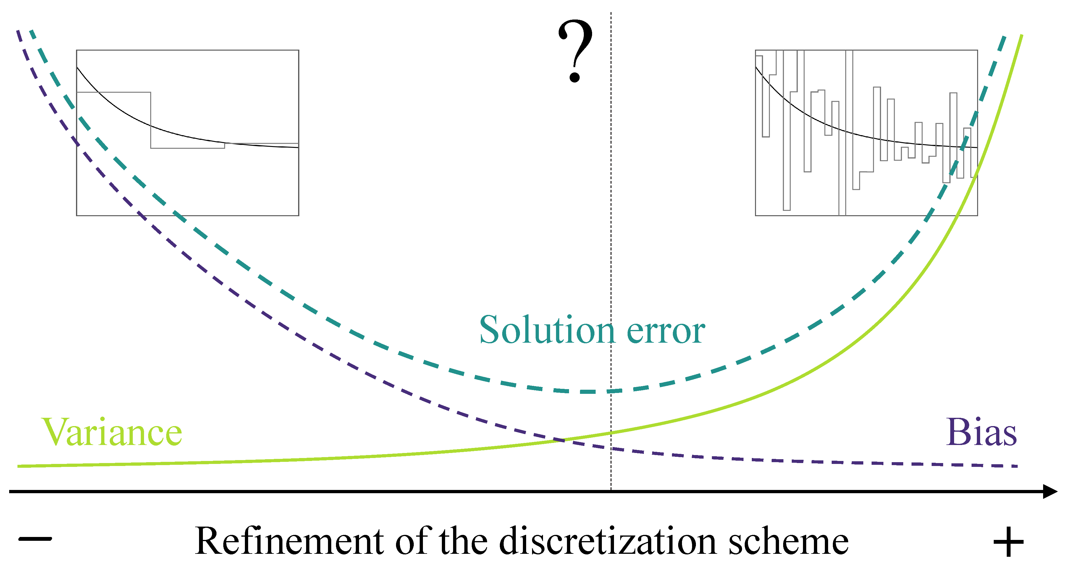
Nonetheless, the most distinctive feature of an ill-posed problem is the varying level of ill-conditioning, which depends on how much the discretized problem closely resembles the original problem. The more it does, the more the obtained problem is ill-conditioned; to tame the ill-conditioning, it is tempting to take coarser discretization with just a few degrees of freedom, but that leads to the solution of a biased problem. Eventually, a so-called bias–variance tradeoff is defined, depicted in Figure 3 and discussed in Section 4 through the proposed numerical experiment.

3. Numerical Investigations

In order to pair the theoretical discussion with a hands-on numerical example, the following tensile residual stress distribution is assumed to be present in a long plate of width W such as the one depicted in Figure 1:
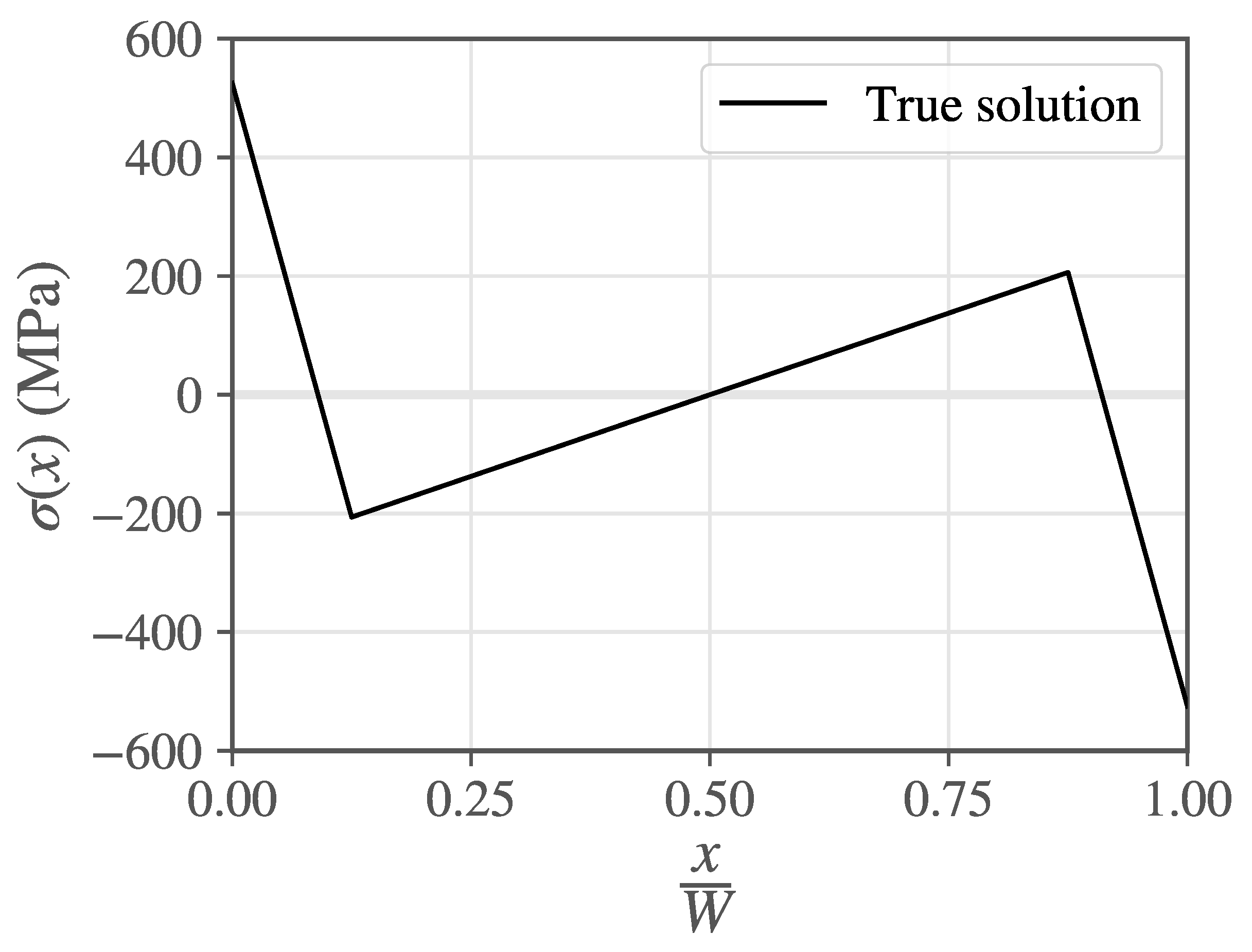
σ ( x ) = 525 5850 x W x W 0.125 275 + 550 x W 0.125 < x W 0.875 5325 5850 x W x W > 0.875 ( MPa )
A plot of the assumed stress distribution is reported in Figure 4. Equation (11) is obtained by carrying out a hypothetical four-point bending test significantly past the yield point of a material having a perfectly plastic constitutive model, and then by removing the applied load, leaving the residual stresses with the task of maintaining the planarity of the section. The problem consists of reconstructing the residual stress distribution in the interval 0 < x W 0.75 through the crack compliance method by introducing a cut in the plate and measuring the CMOD while the cut advances.
The influence function for this problem is taken from [41], which reports it as a truncated series expansion:
h ( a , x ) = 1 2 π a k = 1 5 F a W , k 1 x a k 3 2
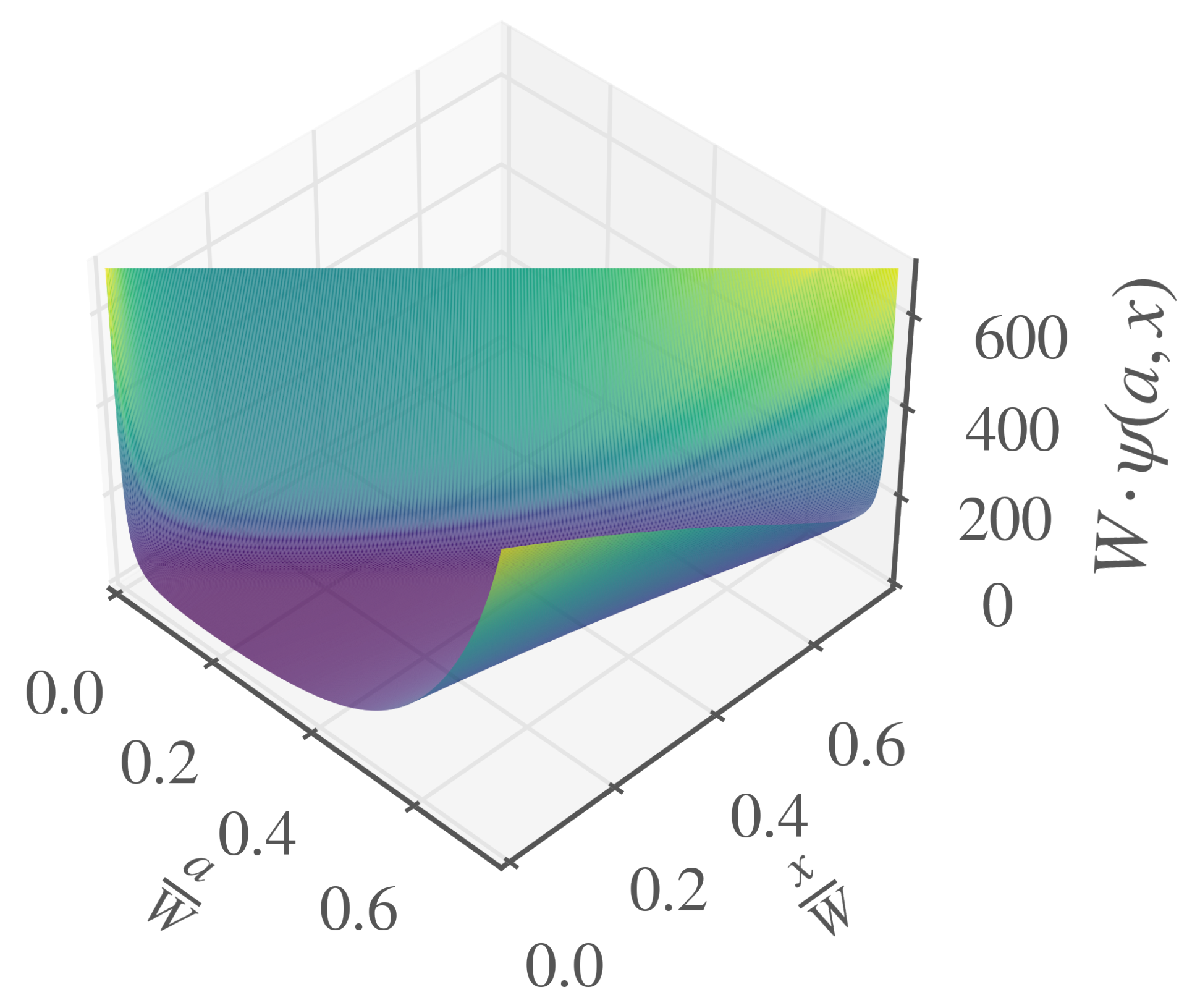
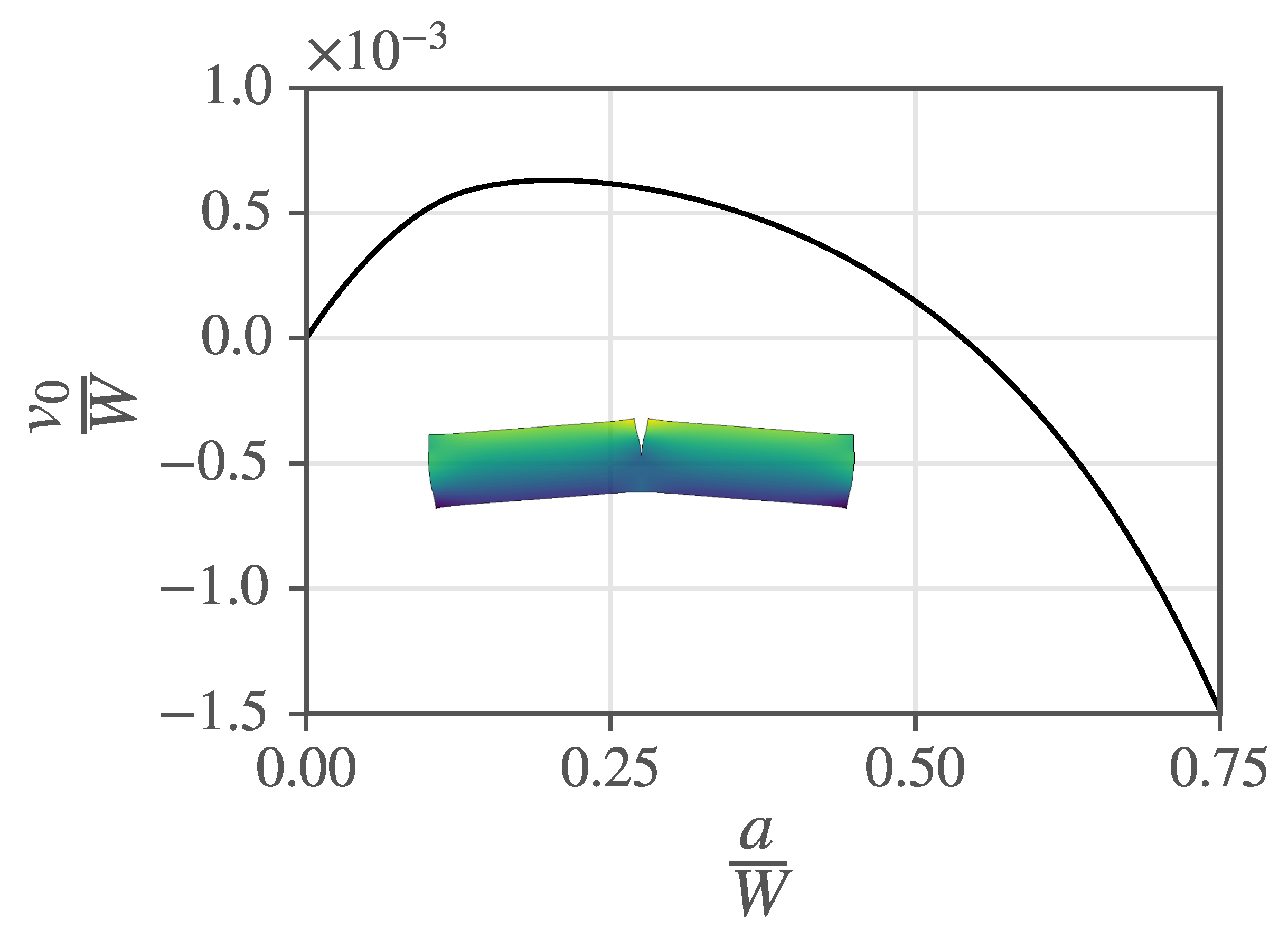
where F a W , k is a dimensionless algebraic function, whose coefficients are tabulated in the book. The corresponding kernel function ψ ( a , x ) = h ( a , 0 ) h ( a , x ) of the integral operator in Equation (8) is reported in Figure 5. By including Equations (11) and (12) in Equation (8), one obtains the theoretical CMOD 2 v 0 ( a ) as a function of the length a of the cut that has been introduced in the specimen, as shown in Figure 6.
As ψ ( a , x ) is available in closed form, Equation (8) allows for the calculation of the CMOD corresponding to any distribution of relaxed residual stresses σ ( x ) through a double integration of a function, an operation that can also be carried out by hand, analytically. Yet, the practical problem lies in measuring v 0 ( a ) and finding σ ( x ) , which involves an inversion of the operator defined by Equation (8). Unfortunately, with a few rare exceptions, an analytical expression of this inverse relationship—that is, a closed-form expression that allows for the determination of σ ( x ) from v 0 ( a ) , is generally not available. As a consequence, the scheme of Figure 2 is also adopted here.
A finite-dimensional stress space spanned by a suitable basis is chosen, then the calibration matrix for the discretized problem is computed by evaluating the CMOD corresponding to the elements of the stress basis at a fixed number of cut lengths. The only difference with the usual state of the art of the slitting method is that here this operation can be carried out analytically, without resorting to FE analyses. In formal terms, if β = β 1 ( z ) , β 2 ( z ) β n ( z ) is the chosen n-dimensional basis and a = a 1 , a 2 a m is the vector of m cut lengths where the CMOD is probed, one can define a matrix
A i j = 0 a i 0 s ψ ( s , t ) β j ( t ) d t d s
so that, for a given residual stress distribution σ ( x ) = j = 1 n σ j β j ( x ) , the following relation holds:
v ( a i , 0 ) = 0 a i 0 s ψ ( s , t ) σ ( t ) d t d s = 0 a i 0 s ψ ( s , t ) j = 1 n σ j β j ( t ) d t d s = j = 1 n σ j 0 a i 0 s ψ ( s , t ) β j ( t ) = j = 1 n A i j σ j
By recording the measured CMODs in an array v = v ( a 1 , 0 ) , v ( a 2 , 0 ) v ( a m , 0 ) and collecting the coordinates of the residual stress distribution with respect to the chosen basis σ = σ 1 , σ 2 σ n , a linear system is obtained, which represents the discretization of Equation (8):
A σ = v
Finally, Equation (15) is generally solved in a least-squares sense by looking for the solution that best approximates the recorded measurement samples. In fact, it is fairly common to exploit the statistical advantages of having more sampling points than strictly necessary [16].
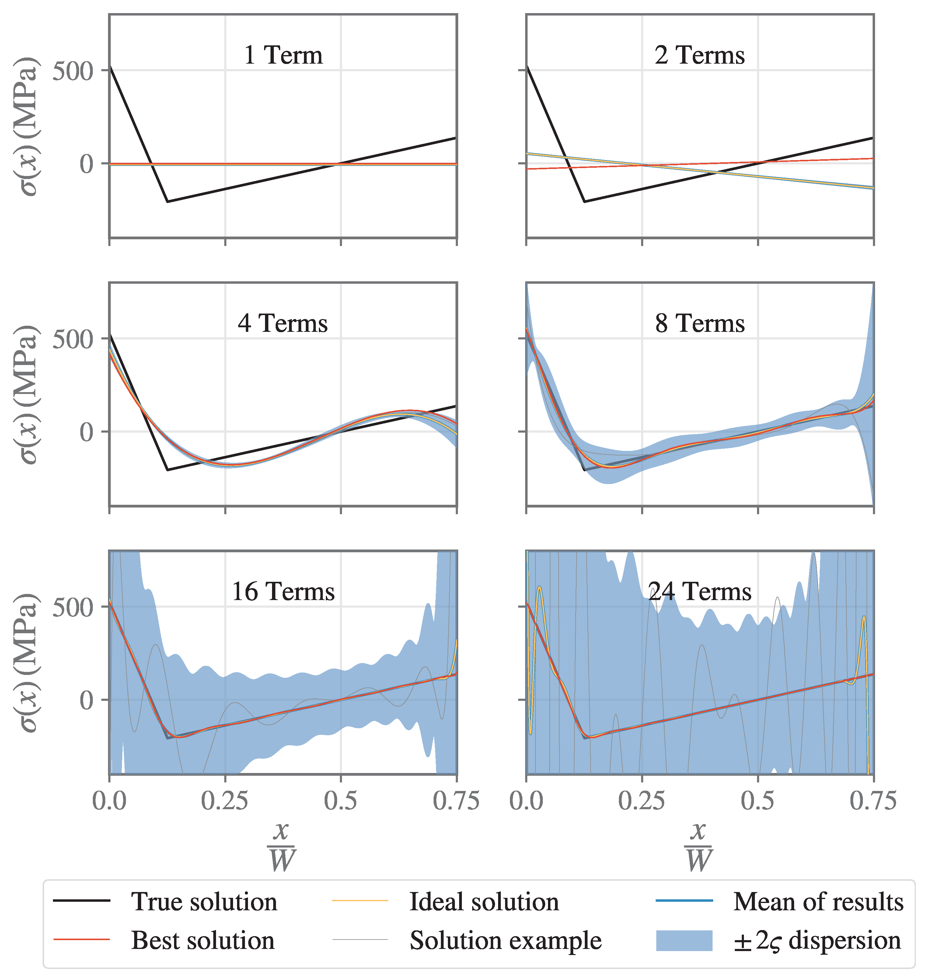
In this analysis, two different stress spaces are employed, owing to their wide application in the residual stress community: the space of piecewise constant functions and the space of polynomials, which, respectively, are usually referred to as the Integral Method [21] and the Power Series Method [42]. To explore the bias–variance tradeoff, a fixed number of 32 probed cut lengths is assumed, while the stress basis dimension is varied between 1 and 32; for the Integral Method, this is performed by increasing the number of calculation intervals, whereas for the Power Series Method, this is performed by adding higher-order terms in the polynomial expansion.
Just for the numerical calculations, a W = 20 mm is adopted, while the standard error of the CMOD measuring instrument is assumed to be 1 μ m . The true CMOD—evaluated through the direct application of Equation (8)—is then sampled at the probed cut lengths and perturbed with a i.i.d. Gaussian noise having a standard deviation equal to the assumed error. In total, 1000 random perturbations of the true CMOD are sampled, and an equal number of results in terms of identified residual stresses is obtained. Moreover, for each discretization scheme, two additional solutions are computed:
  • The ideal solution, which is the one corresponding to perfect, errorless CMOD measurements.
  • The best solution, which is the element of the chosen stress basis that best approximates the true solution in a least-squares sense.
All the results are collected in Figure 7 and Figure 8, respectively corresponding to the application of the Integral Method and the Power Series Method.

4. Discussion

Figure 7 and Figure 8 illustrate the clearest symptom of the ill-posedness of an inverse problem. When the number of degrees of freedom in the finite-dimensional discretization is low, the sensitivity to errors is small, and the solutions are substantially independent of measurement noise. However, the chosen basis is not capable of correctly representing the true solution, so the obtained result shows a bias—potentially dangerous when structural safety is involved—relative to the exact result. As noted in [27], the situation does not change even when the obtained solution is interpreted as the best representation of the exact result within the chosen basis, which, in the case of the Integral Method, would coincide with the average of the true solution over a calculation subinterval. As shown in the figures, even the solution corresponding to errorless measurements is biased with respect to the best representation of the exact result in the chosen finite-dimensional space.
In an attempt to reduce bias, the number of degrees of freedom may be increased so that the finite-dimensional solution is a practically reasonable approximation of the original infinite-dimensional space. Nonetheless, in turn, this yields an inversion process that is extremely sensitive to measurement errors, hence a solution variance that makes every obtained result practically unusable. This has long been known in the literature, also concerning other relaxation methods that do not necessarily require the introduction of a crack-like cut in the specimen [43,44,45]. In intuitive terms, having more degrees of freedom makes the discretized problem closer to its originally ill-posed counterpart, which has an infinite sensitivity to input errors. Note that this effect does not depend on imperfect knowledge of the integral operator—as is the case when it is estimated numerically [46]—because in this example, the operator of the direct problem is known analytically. This is the main reason why the crack compliance method is particularly instructive in these aspects; nonetheless, similar considerations could have been made for the layer-removal method [13] and for Sachs boring method [12], whose integration kernel is analytically known.
As is depicted in Figure 3, the greatest issue concerning ill-posedness is that bias is not observable. By computing multiple solutions—as performed in this case—one can note the variability in the solution with respect to the input error. Due to the linearity of Equation (15), the input errors can also be theoretically propagated through the inversion procedure. However, one can never know the bias that is being introduced by the chosen solution procedure; for example, a given constant solution may equally correspond to an actually constant true residual stress solution or to an arbitrarily varying distribution that causally yields the same discretized solution.
This aspect is particularly dramatic for constructing confidence intervals for the solution. Only the confidence intervals relative to the ideal solution (i.e., corresponding to perfect measurements) can be constructed, but the practical interest of this construction is essentially null, as it is not even guaranteed that the ideal solution coincides with the best approximation of the true solution in the chosen space. The risk is that, in an effort to achieve narrower confidence intervals, the analyst may implicitly choose to increase the bias of the obtained solution, without this being apparent in the results.
There exist also alternative techniques that aim to regularize the problem; that is, to reduce the variance of the solution. The most notable one is arguably Tikhonov regularization [47,48,49]. However, neither of these techniques are immune to the bias–variance tradeoff, as discussed in [26,27]. As a matter of fact, they also introduce a bias into the solution, which cannot be quantified a priori.
There is only one solution to the issues generated by the ill-posedness of an inverse problem and its resulting bias–variance tradeoff: obtaining additional information through physics, which is capable of establishing a priori that the solution must have a specific form and/or meet certain well-defined constraints. Note that this piece of information cannot be deduced by the mathematical equations alone. Only in that case, by assuming a finite-dimensional solution space that adheres to those conditions, no bias is introduced, and any quantification of uncertainties can be considered rigorous. This is equivalent to asserting that the sensitivity to error should not drive the choice of the discretization scheme; rather, it should be the opposite. Physical assumptions determine the discretization scheme, which then yields its corresponding sensitivity to input errors and establishes requirements for the measurement instruments. If these requirements are impossible to meet, the measurement is not feasible from an engineering standpoint.
For example, if something allows the stress analyst to assert that the distribution of residual stresses is reasonably linear through the thickness—possibly caused by the restoration of far-field incompatibilities in the displacement field of a slender beam—there is no bias in assuming that the solution belongs to the space of first-degree polynomial functions, and the variance associated with such a low number of degrees of freedom is generally rather limited.

5. Conclusions

The main points of the article are outlined below:
  • The ill-posedness of the problem of reconstructing residual stresses from measurements of crack opening displacement following a progressive cut introduced in the specimen is demonstrated and clearly distinguished from its more general property of being ill-conditioned.
  • Through a numerical example, the typical indicator of an ill-posed problem, namely the bias–variance tradeoff, is presented, together with its potentially devastating consequences on the ability to rigorously quantify uncertainties. Therefore, it is extremely important to recognize its presence and avoid actions that only seemingly improve the quality of the solution.
  • As stressed in the authors’ previous works, it is again underlined that no mathematical machinery can permanently overcome the infinite sensitivity to input errors that is inherent to ill-posed problems. The solution is to be found in the physics of the problem, aiming at pieces of information that would allow one to tame the solution variance without introducing significant and, above all, uncomputable biases.

Author Contributions

Conceptualization: M.B. and T.G.; Methodology: M.B. and T.G.; Investigation: M.B. and T.G.; Writing—Original Draft: T.G.; Writing—Review & Editing: M.B.; Supervision: M.B. All authors have read and agreed to the published version of the manuscript.

Funding

This research received no external funding.

Institutional Review Board Statement

Not applicable.

Informed Consent Statement

Not applicable.

Data Availability Statement

The original contributions presented in the study are included in the article, further inquiries can be directed to the corresponding author.

Conflicts of Interest

The authors declare no conflicts of interest.

Correction Statement

This article has been republished with a minor correction to the Data Availability Statement Statement. This change does not affect the scientific content of the article.

Abbreviations

The following abbreviations are used in this manuscript:
CMODCrack mouth opening displacement
FEFinite element
SIFStress intensity factor
WFWeight function

References

  1. Timoshenko, S. History of Strength of Materials: With a Brief Account of the History of Theory of Elasticity and Theory of Structures; Courier Corporation: North Chelmsford, MA, USA, 1983. [Google Scholar]
  2. Schajer, G.S.; Winiarski, B.; Withers, P.J. Hole-Drilling Residual Stress Measurement with Artifact Correction Using Full-Field DIC. Exp. Mech. 2013, 53, 255–265. [Google Scholar] [CrossRef]
  3. Baldi, A. Residual Stress Measurement Using Hole Drilling and Integrated Digital Image Correlation Techniques. Exp. Mech. 2014, 54, 379–391. [Google Scholar] [CrossRef]
  4. Harrington, J.S.; Schajer, G.S. Measurement of Structural Stresses by Hole-Drilling and DIC. Exp. Mech. 2017, 57, 559–567. [Google Scholar] [CrossRef]
  5. Hagara, M.; Trebuňa, F.; Pástor, M.; Huňady, R.; Lengvarský, P. Analysis of the aspects of residual stresses quantification performed by 3D DIC combined with standardized hole-drilling method. Measurement 2019, 137, 238–256. [Google Scholar] [CrossRef]
  6. Salehi, S.D.; Rastak, M.A.; Shokrieh, M.M.; Barrallier, L.; Kubler, R. Full-field measurement of residual stresses in composite materials using the incremental slitting and digital image correlation techniques. Exp. Mech. 2020, 60, 1239–1250. [Google Scholar] [CrossRef]
  7. Petzing, J.N.; Tyrer, J.R. Recent developments and applications in electronic speckle pattern interferometry. J. Strain Anal. Eng. Des. 1998, 33, 153–169. [Google Scholar] [CrossRef]
  8. Schajer, G.S.; Steinzig, M. Full-field calculation of hole drilling residual stresses from electronic speckle pattern interferometry data. Exp. Mech. 2005, 45, 526–532. [Google Scholar] [CrossRef]
  9. Gubbels, W.L.; Schajer, G.S. Development of 3-D Digital Image Correlation Using a Single Color-Camera and Diffractive Speckle Projection. Exp. Mech. 2016, 56, 1327–1337. [Google Scholar] [CrossRef]
  10. Schajer, G.S.; Prime, M.B.; Withers, P.J. Why Is It So Challenging to Measure Residual Stresses? Exp. Mech. 2022, 62, 1521–1530. [Google Scholar] [CrossRef]
  11. Noyan, I.C.; Cohen, J.B. Residual Stress: Measurement by Diffraction and Interpretation; Springer: Berlin/Heidelberg, Germany, 2013. [Google Scholar]
  12. Sachs, G.; Espey, G. The measurement of residual stresses in metal. Iron Age 1941, 148, 148. [Google Scholar]
  13. Treuting, R.G.; Read, W.T. A Mechanical Determination of Biaxial Residual Stress in Sheet Materials. J. Appl. Phys. 1951, 22, 130–134. [Google Scholar] [CrossRef]
  14. Beaney, E.M. Accurate measurement of residual stress on any steel using the centre hole method. Strain 1976, 12, 99–106. [Google Scholar] [CrossRef]
  15. Schajer, G.S. Application of Finite Element Calculations to Residual Stress Measurements. J. Eng. Mater. Technol. 1981, 103, 157–163. [Google Scholar] [CrossRef]
  16. Prime, M.B. Residual Stress Measurement by Successive Extension of a Slot: The Crack Compliance Method. Appl. Mech. Rev. 1999, 52, 75–96. [Google Scholar] [CrossRef]
  17. Prime, M.B. Cross-Sectional Mapping of Residual Stresses by Measuring the Surface Contour After a Cut. J. Eng. Mater. Technol. 2001, 123, 162–168. [Google Scholar] [CrossRef]
  18. Schajer, G.S. Practical Residual Stress Measurement Methods; John Wiley & Sons: Hoboken, NJ, USA, 2013. [Google Scholar]
  19. Schajer, G.S. Hole Eccentricity Correction for Hole-Drilling Residual Stress Measurements. Exp. Mech. 2022, 62, 1603–1613. [Google Scholar] [CrossRef]
  20. Bueckner, H.F. Novel principle for the computation of stress intensity factors. Z. Fuer Angew. Math. Mech. 1970, 50, 529–546. [Google Scholar]
  21. Schajer, G.S.; Prime, M.B. Use of Inverse Solutions for Residual Stress Measurements. J. Eng. Mater. Technol. 2006, 128, 375. [Google Scholar] [CrossRef]
  22. Schajer, G.S. Measurement of Non-Uniform Residual Stresses Using the Hole-Drilling Method. Part I Stress Calculation Procedures. J. Eng. Mater. Technol. 1988, 110, 338–343. [Google Scholar] [CrossRef]
  23. Schajer, G.S. Measurement of Non-Uniform Residual Stresses Using the Hole-Drilling Method. Part II Practical Application of the Integral Method. J. Eng. Mater. Technol. 1988, 110, 344–349. [Google Scholar] [CrossRef]
  24. Schajer, G.S.; Prime, M.B. Residual stress solution extrapolation for the slitting method using equilibrium constraints. J. Eng. Mater. Technol. 2007, 129, 227–232. [Google Scholar] [CrossRef]
  25. Schajer, G.S.; Altus, E. Stress Calculation Error Analysis for Incremental Hole-Drilling Residual Stress Measurements. J. Eng. Mater. Technol. 1996, 118, 120–126. [Google Scholar] [CrossRef]
  26. Beghini, M.; Grossi, T.; Prime, M.; Santus, C. Ill-Posedness and the Bias-Variance Tradeoff in Residual Stress Measurement Inverse Solutions. Exp. Mech. 2023, 63, 495–516. [Google Scholar] [CrossRef]
  27. Beghini, M.; Grossi, T. Towards a Reliable Uncertainty Quantification in Residual Stress Measurements with Relaxation Methods: Finding Average Residual Stresses is a Well-Posed Problem. Exp. Mech. 2024, 64, 851–874. [Google Scholar] [CrossRef]
  28. Beghini, M.; Bertini, L.; Cococcioni, M.; Grossi, T.; Santus, C.; Benincasa, A. Regularization of Hole-Drilling Residual Stress Measurements with Eccentric Holes: An Approach with Influence Functions. J. Mater. Eng. Perform. 2024, 1–7. [Google Scholar] [CrossRef]
  29. Beghini, M.; Grossi, T.; Santus, C. Validation of a strain gauge rosette setup on a cantilever specimen: Application to a calibration bench for residual stresses. Mater. Today Proc. 2023, 93, 719–724. [Google Scholar] [CrossRef]
  30. Beghini, M.; Grossi, T.; Santus, C.; Valentini, E. A calibration bench to validate systematic error compensation strategies in hole drilling measurements. In Proceedings of the ICRS 11–11th International Conference on Residual Stresses, Nancy, France, 27–30 March 2022. [Google Scholar] [CrossRef]
  31. Beghini, M.; Grossi, T.; Santus, C.; Seralessandri, L.; Gulisano, S. Residual stress measurements on a deep rolled aluminum specimen through X-Ray Diffraction and Hole-Drilling, validated on a calibration bench. IOP Conf. Ser. Mater. Sci. Eng. 2023, 1275, 012036. [Google Scholar] [CrossRef]
  32. Cheng, W.; Finnie, I. Residual Stress Measurement and the Slitting Method; Mechanical Engineering Series; Springer: New York, NY, USA, 2007. [Google Scholar]
  33. Vaidyanathan, S.; Finnie, I. Determination of Residual Stresses From Stress Intensity Factor Measurements. J. Basic Eng. 1971, 93, 242–246. [Google Scholar] [CrossRef]
  34. Schindler, H.J.; Cheng, W.; Finnie, I. Experimental determination of stress intensity factors due to residual stresses. Exp. Mech. 1997, 37, 272–277. [Google Scholar] [CrossRef]
  35. Anderson, T.L. Fracture Mechanics: Fundamentals and Applications; CRC Press: Boca Raton, FL, USA, 2017. [Google Scholar]
  36. Rice, J.R. Some remarks on elastic crack-tip stress fields. Int. J. Solids Struct. 1972, 8, 751–758. [Google Scholar] [CrossRef]
  37. Lamm, P.K. A Survey of Regularization Methods for First-Kind Volterra Equations. In Surveys on Solution Methods for Inverse Problems; Colton, D., Engl, H.W., Louis, A.K., McLaughlin, J.R., Rundell, W., Eds.; Springer: Vienna, Austria, 2000; pp. 53–82. [Google Scholar]
  38. von Mises, R. On Saint Venant’s principle. Bull. Am. Math. Soc. 1945, 51, 555–562. [Google Scholar] [CrossRef]
  39. Goldberg, R.R. Methods of Real Analysis; Oxford and IBH Publishing: Delhi, India, 1970. [Google Scholar]
  40. Rudin, W. Real and Complex Analysis, 3rd ed.; McGraw-Hill: New York, NY, USA, 1987. [Google Scholar]
  41. Wu, X.R.; Carlsson, J. Weight Functions and Stress Intensity Factor Solutions; Pergamon Press: Oxford, UK, 1991. [Google Scholar]
  42. Prime, M.B.; Hill, M.R. Uncertainty, Model Error, and Order Selection for Series-Expanded, Residual-Stress Inverse Solutions. J. Eng. Mater. Technol. 2006, 128, 175–185. [Google Scholar] [CrossRef]
  43. Zuccarello, B. Optimal calculation steps for the evaluation of residual stress by the incremental hole-drilling method. Exp. Mech. 1999, 39, 117–124. [Google Scholar] [CrossRef]
  44. Zuccarello, B. Optimization of depth increment distribution in the ring-core method. J. Strain Anal. Eng. Des. 1996, 31, 251–258. [Google Scholar] [CrossRef]
  45. Olson, M.D. Measurement Layout for Residual Stress Mapping Using Slitting. Exp. Mech. 2022, 62, 393–402. [Google Scholar] [CrossRef]
  46. Schajer, G.S. Compact Calibration Data for Hole-Drilling Residual Stress Measurements in Finite-Thickness Specimens. Exp. Mech. 2020, 60, 665–678. [Google Scholar] [CrossRef]
  47. Tikhonov, A.N.; Goncharsky, A.V.; Stepanov, V.V.; Yagola, A.G. Numerical Methods for the Solution of Ill-Posed Problems; Springer: Dordrecht, The Netherlands, 1995. [Google Scholar] [CrossRef]
  48. Schajer, G.S. Hole-Drilling Residual Stress Profiling with Automated Smoothing. J. Eng. Mater. Technol. 2007, 129, 440–445. [Google Scholar] [CrossRef]
  49. Smit, T.C.; Reid, R. Tikhonov Regularization for the Fully Coupled Integral Method of Incremental Hole-Drilling. Exp. Mech. 2024, 64, 275–290. [Google Scholar] [CrossRef]
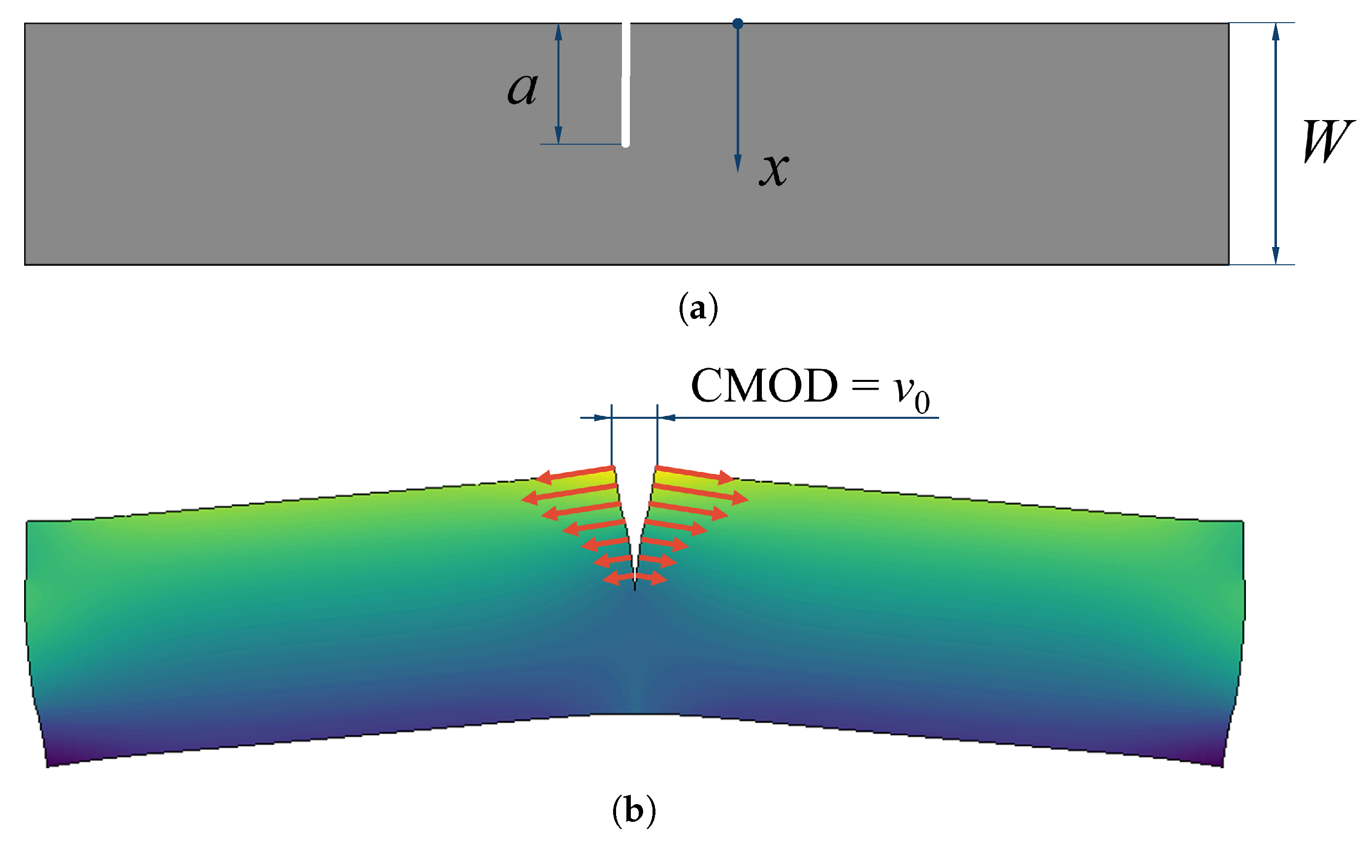
Figure 1. A classical application of Bueckner’s superposition principle. A cut is introduced in a specimen in a region where tensile residual stresses are present. This action generates displacement fields that are equivalent to those obtained with the simple elastic boundary problem depicted in the figure, where the applied tractions are simply reversed in sign. (a): Naming of geometrical variables: crack length a, spatial coordinate x and specimen width W. (b): Equivalent boundary value problem, color-coded by the magnitude of displacements along the crack face normal. Tractions are represented as red arrows.
Applmech 05 00027 g001
Figure 2. Standard procedure used to build the calibration matrix in a discretized version of Equation (1). For each element of the chosen stress basis—which in this case spans the set of piecewise constant stress distributions—the corresponding displacements or strains arising from a hypothetical run of the same measuring process are simulated and recorded as columns of the calibration matrix. Then, leveraging the superposition principle of linear elasticity, the displacements/strains corresponding to any element of the chosen stress space can be simulated through a linear combination of the columns of the calibration matrix. Each element of the stress basis is represented with a different color.
Applmech 05 00027 g002
Figure 3. Pictorial representation of the bias–variance tradeoff, typically faced by the residual stress analyst when choosing the discretization scheme. As the number of degrees of freedom allowed in the basis spanning the stresses increases, the variance of the solution (light green curve) increases in terms of sensitivity to measurement errors. In an attempt to reduce this sensitivity by limiting the degrees of freedom, a bias (blue curve) is introduced into the solution. If both the variance and the bias were observable, the discretization scheme that generates the “best” solution (i.e., the minimum of the turquoise curve) could be chosen; however, bias is not directly observable.
Applmech 05 00027 g003
Figure 4. Residual stress distribution used in the proposed numerical experiment, defined by Equation (11).
Applmech 05 00027 g004
Figure 5. Plot of the kernel function ψ ( a , x ) , used to calculate the CMOD from knowledge of the residual stresses along the introduced crack, through a double integration. Having units of 1 / Length , it is normalized by 1 / W . The kernel function is defined on the triangular domain 0 x < a < W , and it has an integrable singularity along its diagonal x = a . The X and Y coordinates are normalized by the specimen width; in the plot, both a and x are limited to 0.75 W, consistently with the proposed numerical experiment. The surface plot is color-coded according to the Z coordinate.
Applmech 05 00027 g005
Figure 6. Normalized CMOD that corresponds to the residual stress distribution defined by Equation (11), following a progressive cut of normalized length a / W < 0.75 in a long plate in plane strain. Since the introduced cut has a non-null thickness, a negative CMOD is allowed and does not automatically generate crack closure. The specimen is color-coded by the magnitude of displacements along the crack face normal.
Applmech 05 00027 g006
Figure 7. Results of the numerical experiments, obtained by employing the finite-dimensional stress space consisting of piecewise constant functions. In total, 1000 random perturbations of the theoretical CMOD corresponding to σ ( x ) defined by Equation (11) are generated, then the residual stress solutions are identified by inverting the linear system reported in Equation (15). The best solution is the one that best approximates the true solution; the ideal solution is the one that would be obtained with errorless measurements. For low-dimensional discretizations, the variance of the obtained solution is small, but the stress space itself is not able to represent the true solution, thereby introducing a bias; moreover, the ideal solution does not even match the best one. For high-dimensional discretizations, the ideal solution converges to the true one, but the distribution of obtained solutions has a practically unusable variance.
Applmech 05 00027 g007
Figure 8. Results of the numerical experiments, obtained by employing the finite-dimensional stress space consisting of polynomials. In total, 1000 random perturbations of the theoretical CMOD corresponding to σ ( x ) defined by Equation (11) are generated, then the residual stress solutions are identified by inverting the linear system reported in Equation (15). The best solution is the one that best approximates the true solution; the ideal solution is the one that would be obtained with errorless measurements. For low-dimensional discretization, the variance of the obtained solution is small, but the stress space itself is not able to represent the true solution, thereby introducing a bias; moreover, the ideal solution does not even match the best one. For high-dimensional discretizations, the ideal solution converges to the true one, but the distribution of obtained solutions has a practically unusable variance.
Applmech 05 00027 g008
Disclaimer/Publisher’s Note: The statements, opinions and data contained in all publications are solely those of the individual author(s) and contributor(s) and not of MDPI and/or the editor(s). MDPI and/or the editor(s) disclaim responsibility for any injury to people or property resulting from any ideas, methods, instructions or products referred to in the content.