Response-Only Damage Detection Approach of CFRP Gas Tanks Using Clustering and Vibrational Measurements


Abstract
:1. Introduction
2. Clustering
2.1. Hierarchical Clustering
- Evaluation of the pairwise distance of the data sets.More details on the calculation of this step are referred to in Section 2.3.
- Construct the hierarchical binary tree.In this step, similar pairs of points are merged into a cluster. Iteratively, these clusters are merged again to construct higher-level clusters until the tree is fully developed. The criterion for merging is the distance metric.Several different methods exist to achieve this procedure, such as the single linkage, complete linkage, and average linkage approaches [39]. In the present work, the complete linkage method is considered. With this method, any point to be included in an existing cluster must be within a certain level of similarity to all members of that cluster.
- 3.
- Cut the tree into the specified number of clusters. The number of clusters is an input variable.
2.2. Spectral Clustering
- Let be the collection of observations, where is the total number of observations, and is a set of variables. Each variable can be a single data point or, with proper modifications, it can be a set of data points. In the context of this work, a variable inside is treated as a collection of data points, as it represents a curve on the frequency domain.
- Using the selected distance function, the pairwise distance () is calculated between all observations.
- Construction of the similarity matrix. Using the matrix, the elements of row and column of the similarity matrix can be calculated using Equation (2). The similarity matrix is the matrix representation of the graph.
- Calculate the unnormalized Laplacian matrix using Equation (3):where , degree matrix, is a diagonal matrix calculated by the sum of the rows of the similarity matrix. As such, the -th diagonal element is calculated using Equation (4).
- Calculate the normalized Laplacian matrix using Equation (5).
- Solve the eigenvalue problem and calculate the first numbers of eigenvectors. Let be the matrix containing the eigenvectors (as columns).
- Use each row of as a point and cluster with the k-means algorithm.
- Finally, group the original points in along with the points of the corresponding row of .
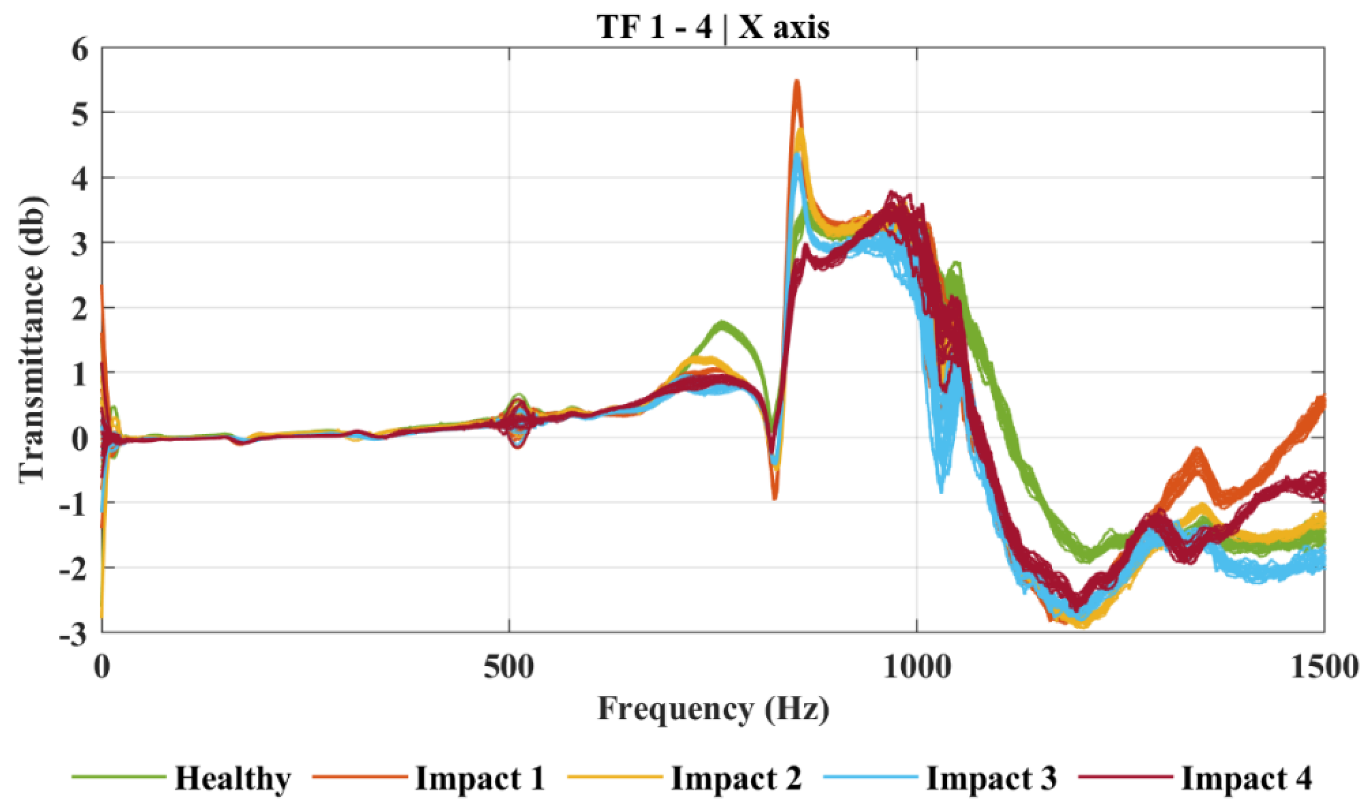
2.3. Metric of Comparison
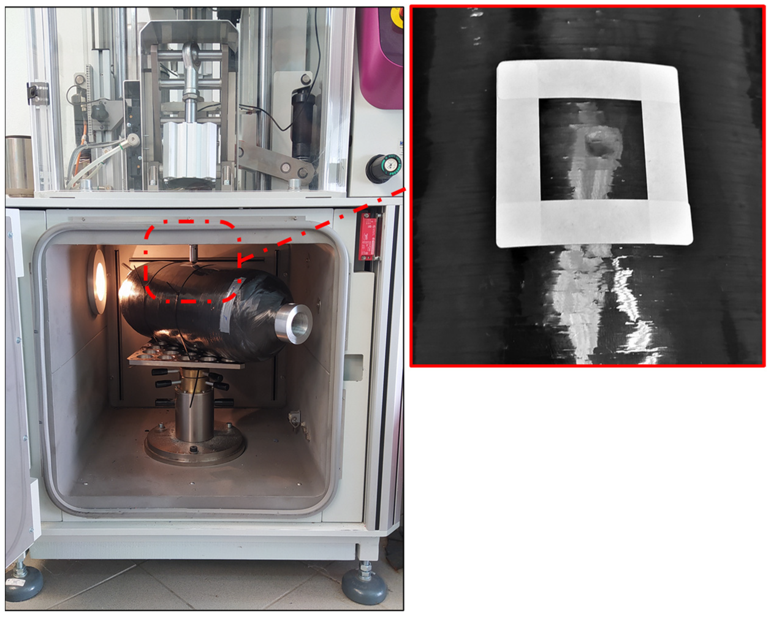
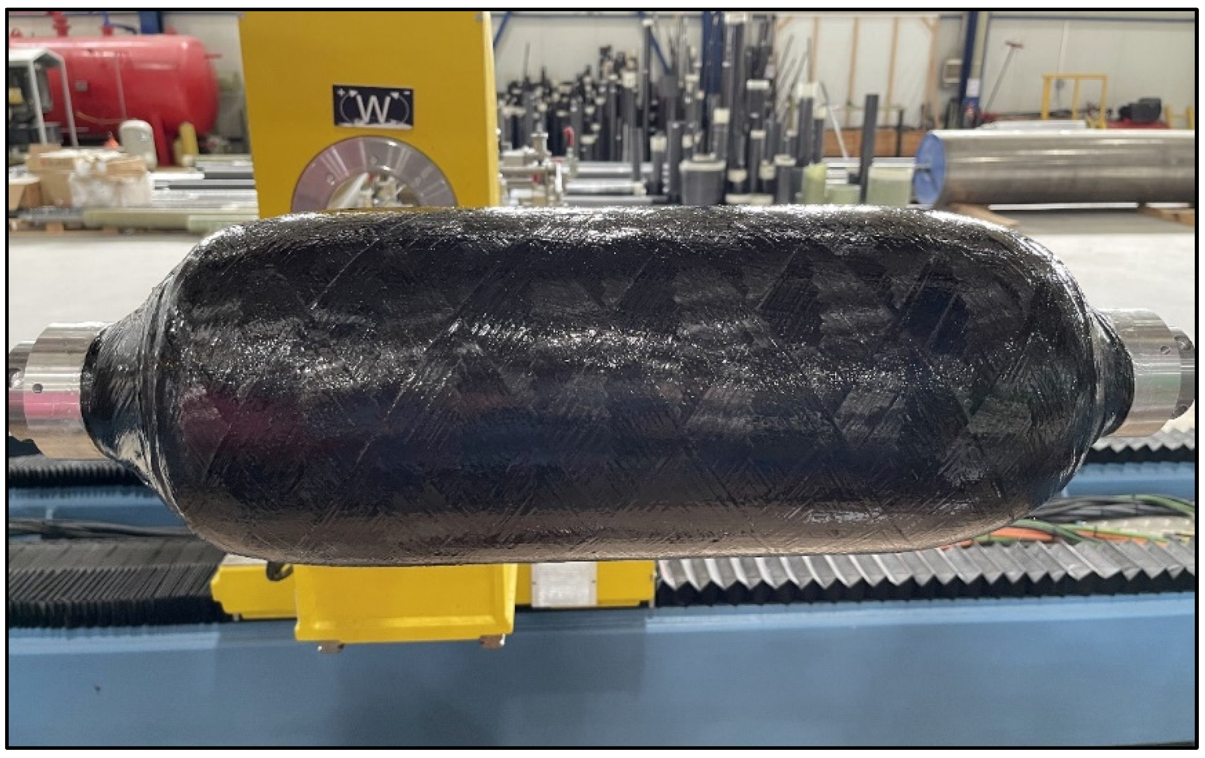
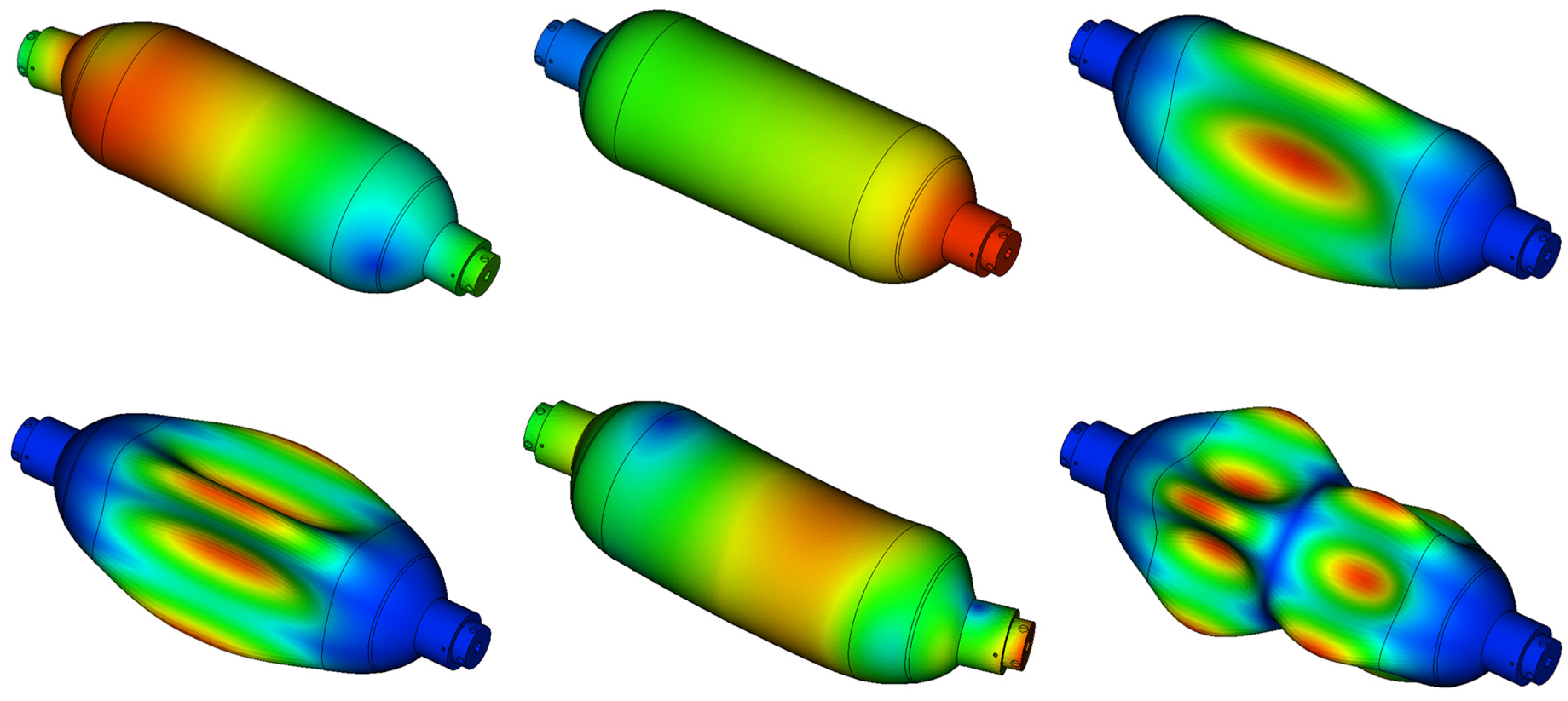
3. Type V CFRP Tank Impact Damage
3.1. Impact Damage
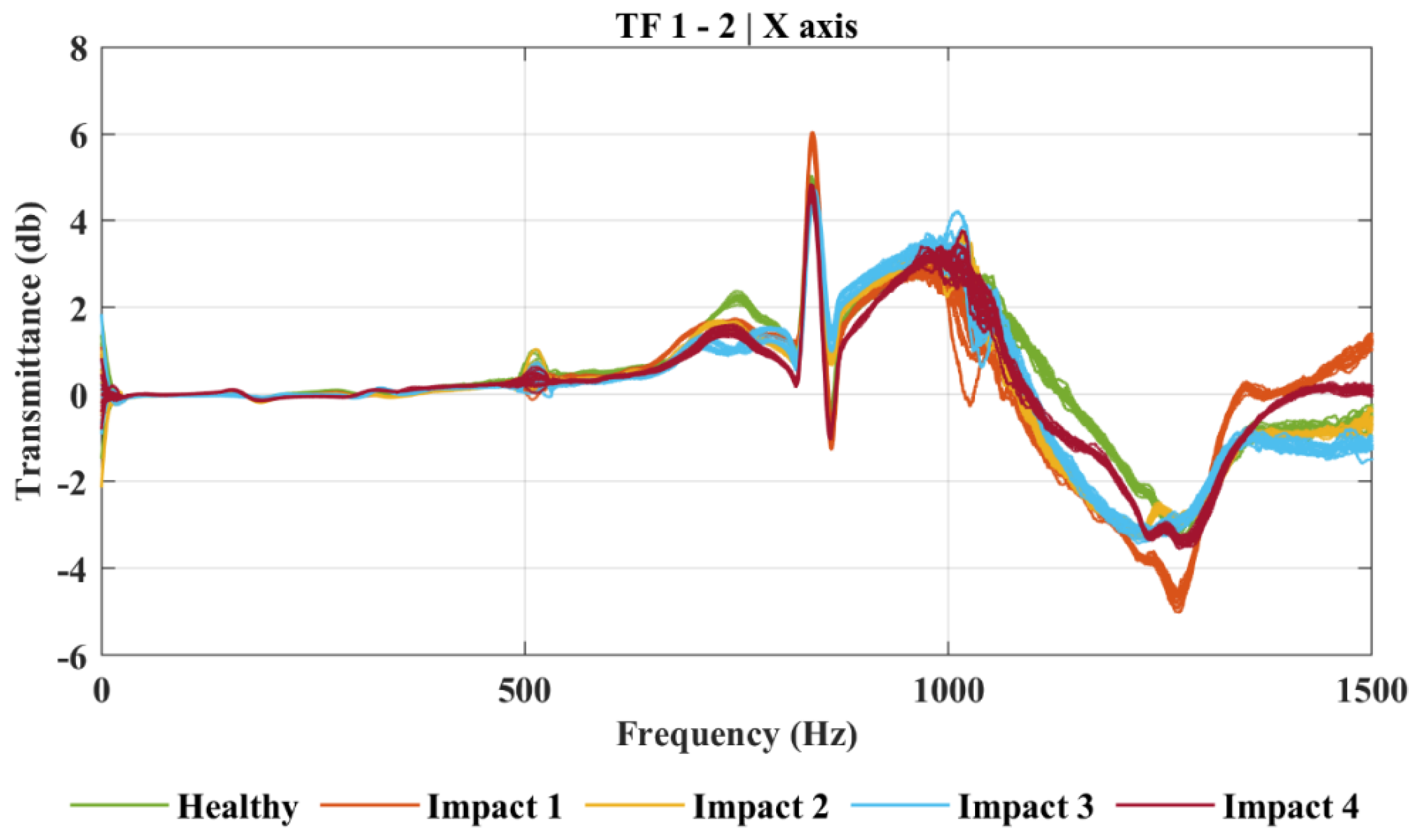
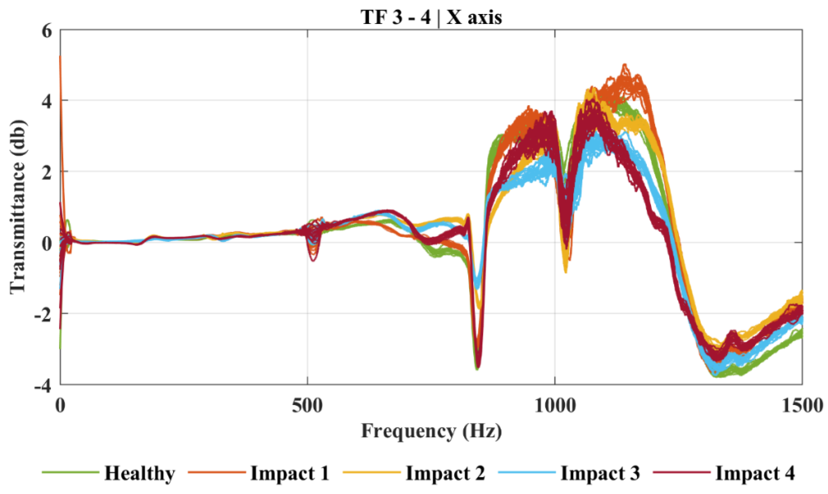
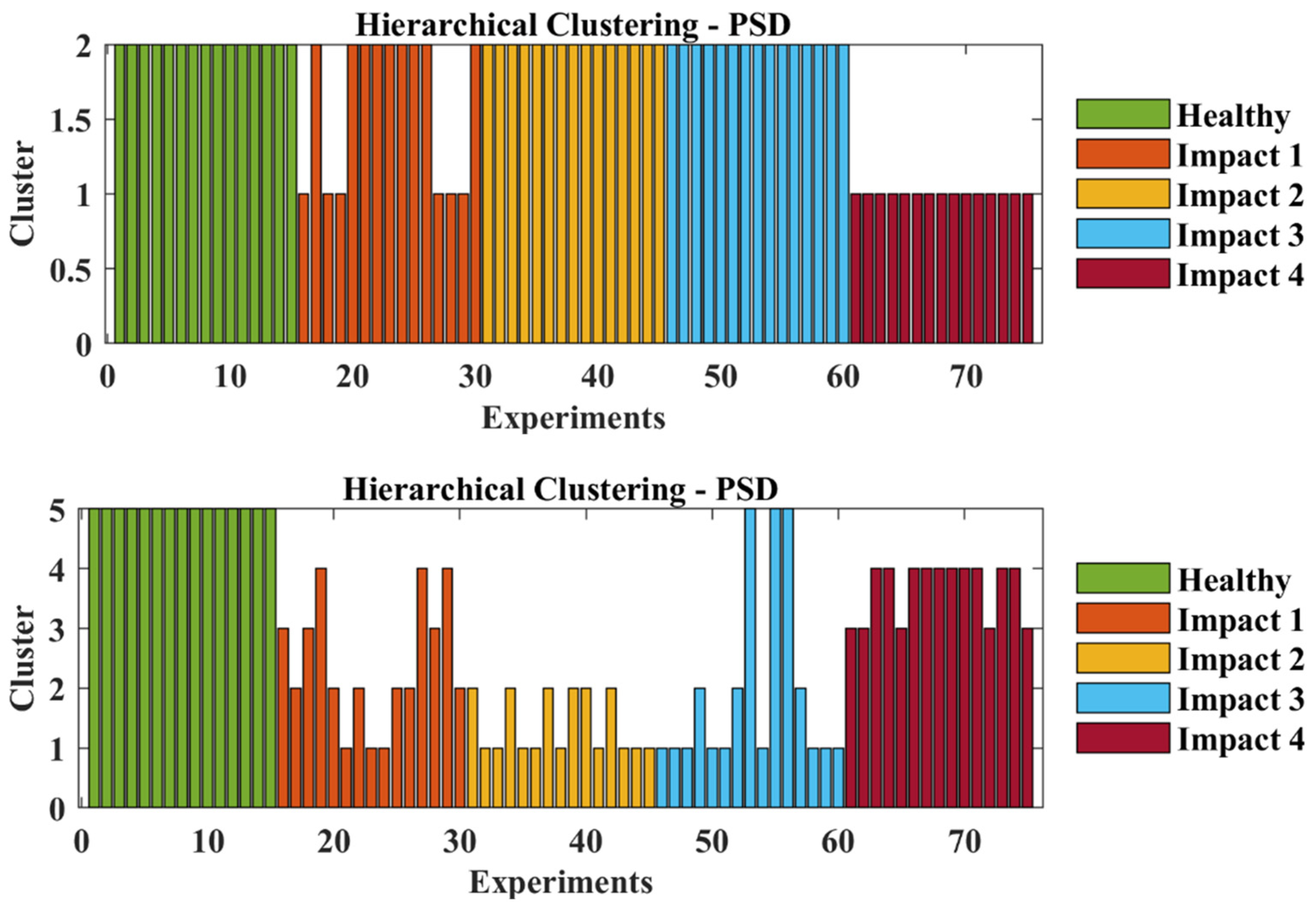
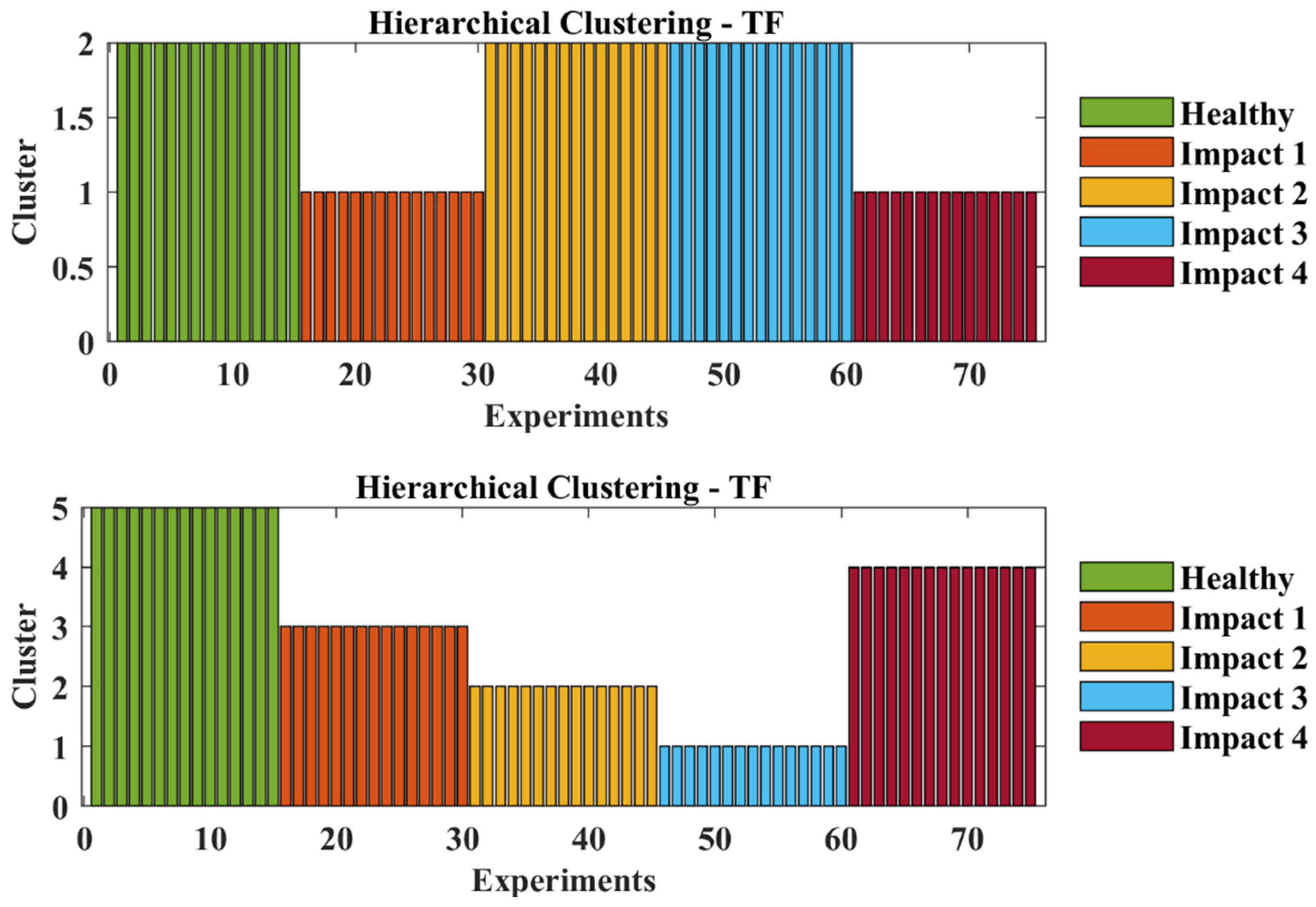
3.2. Clustering
4. Conclusions
Author Contributions
Funding
Institutional Review Board Statement
Informed Consent Statement
Data Availability Statement
Conflicts of Interest
References
- Das, S.; Warren, J.; West, D.; Schexnayder, S.M. Global Carbon Fiber Composites Supply Chain Competitiveness Analysis; Clean Energy Manufacturing Analysis Center: Golden, CO, USA, 2016. [Google Scholar]
- Yamashita, A.; Kondo, M.; Goto, S.; Ogami, N. Development of High-Pressure Hydrogen Storage System for the Toyota “Mirai”; SAE Technical Paper; SAE International: Detroit, MI, USA, 2015. [Google Scholar] [CrossRef]
- Berro Ramirez, J.P.; Halm, D.; Grandidier, J.C.; Villalonga, S.; Nony, F. 700 bar type IV high pressure hydrogen storage vessel burst—Simulation and experimental validation. Int. J. Hydrogen Energy 2015, 40, 13183–13192. [Google Scholar] [CrossRef]
- Robinson, M.; Stolzfus, J.; Owens, T. Composite material compatibility with liquid and gaseous oxygen. In Proceedings of the 19th AIAA Applied Aerodynamics Conference, Anaheim, CA, USA, 11–14 June 2001; American Institute of Aeronautics and Astronautics: Reston, VA, USA, 2001. [Google Scholar]
- Richardson, M.O.W.; Wisheart, M.J. Review of low-velocity impact properties of composite materials. Compos. Part A Appl. Sci. Manuf. 1996, 27, 1123–1131. [Google Scholar] [CrossRef]
- Meola, C.; Carlomagno, G.M. Non-destructive evaluation (NDE) of aerospace composites: Detecting impact damage. In Non-Destructive Evaluation (NDE) of Polymer Matrix Composites; Elsevier: Cambridge, UK, 2013; pp. 367–396. [Google Scholar]
- Bulletti, A.; Giannelli, P.; Calzolai, M.; Capineri, L. An Integrated Acousto/Ultrasonic Structural Health Monitoring System for Composite Pressure Vessels. IEEE Trans. Ultrason. Ferroelectr. Freq. Control 2016, 63, 864–873. [Google Scholar] [CrossRef] [PubMed]
- Huang, J.Q. Non-destructive evaluation (NDE) of composites: Acoustic emission (AE). In Non-Destructive Evaluation (NDE) of Polymer Matrix Composites; Elsevier: Cambridge, UK, 2013; pp. 12–32. [Google Scholar]
- Wong, B.S. Non-destructive evaluation (NDE) of composites: Detecting delamination defects using mechanical impedance, ultrasonic and infrared thermographic techniques. In Non-Destructive Evaluation (NDE) of Polymer Matrix Composites; Elsevier: Cambridge, UK, 2013; pp. 279–308. [Google Scholar]
- Heuer, H.; Schulze, M.H.; Meyendorf, N. Non-destructive evaluation (NDE) of composites: Eddy current techniques. In Non-Destructive Evaluation (NDE) of Polymer Matrix Composites; Elsevier: Cambridge, UK, 2013; pp. 33–55. [Google Scholar]
- Das, S.; Saha, P.; Patro, S.K. Vibration-based damage detection techniques used for health monitoring of structures: A review. J. Civ. Struct. Health Monit. 2016, 6, 477–507. [Google Scholar] [CrossRef]
- Zou, Y.; Tong, L.; Steven, G.P. Vibration-based model-dependent damage (delamination) identification and health monitoring for composite structures—A review. J. Sound Vib. 2000, 230, 357–378. [Google Scholar] [CrossRef]
- Gomes, G.F.; Mendez, Y.A.D.; da Silva Lopes Alexandrino, P.; da Cunha, S.S.; Ancelotti, A.C. A Review of Vibration Based Inverse Methods for Damage Detection and Identification in Mechanical Structures Using Optimization Algorithms and ANN. Arch. Comput. Methods Eng. 2019, 26, 883–897. [Google Scholar] [CrossRef]
- Gomes, G.F.; Mendéz, Y.A.D.; da Cunha, S.S.; Ancelotti, A.C. A numerical–experimental study for structural damage detection in CFRP plates using remote vibration measurements. J. Civ. Struct. Health Monit. 2018, 8, 33–47. [Google Scholar] [CrossRef]
- Zacharakis, I.; Arailopoulos, A.; Markogiannaki, O.; Giagopoulos, D. Damage detection in composite carbon fiber tubes based on experimental measurements and finite element model updating techniques. In Proceedings of the 7th International Conference on Computational Methods in Structural Dynamics and Earthquake Engineering (COMPDYN 2015), Crete, Greece, 24–26 June 2019; Institute of Structural Analysis and Antiseismic Research School of Civil Engineering National Technical University of Athens (NTUA): Athens, Greece, 2019; Volume 2, pp. 2959–2970. [Google Scholar]
- Zacharakis, I.; Arailopoulos, A.; Markogiannaki, O.; Giagopoulos, D. Vibration based structural health monitoring of composite carbon fiber structural systems. In Proceedings of the 3rd International Conference on Uncertainty Quantification in Computational Sciences and Engineering, Uncecomp 2019, Crete, Greece, 24–26 June 2019. [Google Scholar]
- Zacharakis, I.; Giagopoulos, D.; Zyganitidis, I.; Arailopoulos, A.; Markogiannaki, O. Modeling of cfrp structures using model updating techniques and experimental measurements. In Proceedings of the International Conference on Structural Dynamic, EURODYN, Athens, Greece, 23–26 November 2020; Volume 1, pp. 536–550. [Google Scholar]
- Mechbal, N.; Uribe, J.S.; Rébillat, M. A probabilistic multi-class classifier for structural health monitoring. Mech. Syst. Signal Process. 2015, 60–61, 106–123. [Google Scholar] [CrossRef] [Green Version]
- Bull, L.A.; Worden, K.; Dervilis, N. Towards semi-supervised and probabilistic classification in structural health monitoring. Mech. Syst. Signal Process. 2020, 140, 106653. [Google Scholar] [CrossRef]
- Santos, A.; Figueiredo, E.; Silva, M.F.M.; Sales, C.S.; Costa, J.C.W.A. Machine learning algorithms for damage detection: Kernel-based approaches. J. Sound Vib. 2016, 363, 584–599. [Google Scholar] [CrossRef]
- Hou, R.; Xia, Y. Review on the new development of vibration-based damage identification for civil engineering structures: 2010–2019. J. Sound Vib. 2021, 491, 115741. [Google Scholar] [CrossRef]
- Seventekidis, P.; Giagopoulos, D.; Arailopoulos, A.; Markogiannaki, O. Structural Health Monitoring using deep learning with optimal finite element model generated data. Mech. Syst. Signal Process. 2020, 145, 106972. [Google Scholar] [CrossRef]
- Seventekidis, P.; Giagopoulos, D. A combined finite element and hierarchical Deep learning approach for structural health monitoring: Test on a pin-joint composite truss structure. Mech. Syst. Signal Process. 2021, 157, 107735. [Google Scholar] [CrossRef]
- Andriosopoulou, G.; Mastakouris, A.; Vamvoudakis-Stefanou, K.; Fassois, S. Random Vibration Based Robust Damage Detection for a Composite Aerostructure Under Assembly-Induced Uncertainty. In Proceedings of the 13th International Conference on Damage Assessment of Structures, Porto, Portugal, 9–10 July 2019; Lecture Notes in Mechanical Engineering. Springer: Singapore, 2020; pp. 775–787, ISBN 9789811383304. [Google Scholar]
- Pedram, M.; Esfandiari, A.; Khedmati, M.R. Damage detection by a FE model updating method using power spectral density: Numerical and experimental investigation. J. Sound Vib. 2017, 397, 51–76. [Google Scholar] [CrossRef]
- Zhang, H.; Schulz, M.J.; Naser, A.; Ferguson, F.; Pai, P.F. Structural health monitoring using transmittance functions. Mech. Syst. Signal Process. 1999, 13, 765–787. [Google Scholar] [CrossRef]
- Poulimenos, A.G.; Sakellariou, J.S. A transmittance-based methodology for damage detection under uncertainty: An application to a set of composite beams with manufacturing variability subject to impact damage and varying operating conditions. Struct. Health Monit. 2019, 18, 318–333. [Google Scholar] [CrossRef]
- Langone, R.; Reynders, E.; Mehrkanoon, S.; Suykens, J.A.K. Automated structural health monitoring based on adaptive kernel spectral clustering. Mech. Syst. Signal Process. 2017, 90, 64–78. [Google Scholar] [CrossRef] [Green Version]
- Zhou, Y.-L.; Maia, N.M.M.; Sampaio, R.P.C.; Wahab, M.A. Structural damage detection using transmissibility together with hierarchical clustering analysis and similarity measure. Struct. Health Monit. 2017, 16, 711–731. [Google Scholar] [CrossRef]
- Nielsen, F. Introduction to HPC with MPI for Data Science; Undergraduate Topics in Computer Science; Springer International Publishing: Cham, Switzerland, 2016; ISBN 978-3-319-21902-8. [Google Scholar]
- Jain, A.K.; Murty, M.N.; Flynn, P.J. Data clustering: A review. ACM Comput. Surv. 1999, 31, 264–323. [Google Scholar] [CrossRef]
- Aldenderfer, M.; Blashfield, R. Cluster Analysis; SAGE Publications, Inc.: Thousand Oaks, CA, USA, 1984; ISBN 9780803923768. [Google Scholar]
- Ng, A.Y.; Jordan, M.I.; Weiss, Y. On Spectral Clustering: Analysis and an Algorithm. In Proceedings of the 14th International Conference on Neural Information Processing Systems: Natural and Synthetic, Vancouver, BC, Canada, 3–8 December 2001; MIT Press: Cambridge, MA, USA, 2001; pp. 849–856. [Google Scholar]
- Meilua, M.; Shi, J. A Random Walks View of Spectral Segmentation. In Proceedings of the Eighth International Workshop on Artificial Intelligence and Statistics, Key West, FL, USA, 4–7 January 2001; Richardson, T.S., Jaakkola, T.S., Eds.; 2001; Volume R3, pp. 203–208. [Google Scholar]
- Shi, J.; Malik, J. Normalized cuts and image segmentation. IEEE Trans. Pattern Anal. Mach. Intell. 2000, 22, 888–905. [Google Scholar] [CrossRef] [Green Version]
- Von Luxburg, U. A tutorial on spectral clustering. Stat. Comput. 2007, 17, 395–416. [Google Scholar] [CrossRef]
- Pedregosa, F.; Varoquaux, G.; Gramfort, A.; Michel, V.; Thirion, B.; Grisel, O.; Blondel, M.; Prettenhofer, P.; Weiss, R.; Dubourg, V.; et al. Scikit-learn: Machine Learning in {P}ython. J. Mach. Learn. Res. 2011, 12, 2825–2830. [Google Scholar]
- The MathWorks Inc. MATLAB 2020. Available online: https://www.mathworks.com/ (accessed on 8 December 2021).
- Roux, M. A Comparative Study of Divisive and Agglomerative Hierarchical Clustering Algorithms. J. Classif. 2018, 35, 345–366. [Google Scholar] [CrossRef] [Green Version]
- Maia, N.M.M.; Almeida, R.A.B.; Urgueira, A.P.V.; Sampaio, R.P.C. Damage detection and quantification using transmissibility. Mech. Syst. Signal Process. 2011, 25, 2475–2483. [Google Scholar] [CrossRef]
- Chesné, S.; Deraemaeker, A. Damage localization using transmissibility functions: A critical review. Mech. Syst. Signal Process. 2013, 38, 569–584. [Google Scholar] [CrossRef] [Green Version]


| Accelerometer | Height (mm) | Angle (Degrees) |
|---|---|---|
| A1 | 240 | 0 |
| A2 | 480 | 135 |
| A3 | 300 | 180 |
| A4 | 420 | 270 |
| Experiment | Impact Energy (Joules) | Vibration Experiments |
|---|---|---|
| Healthy | - | 15 |
| Impact 1 | 10 | 15 |
| Impact 2 | 10 | 15 |
| Impact 3 | 10 | 15 |
| Impact 4 | 10 | 15 |
| Measure | Clustering Method | Cluster Input | Result |
|---|---|---|---|
| Power Spectral Density (PSD) | Hierarchical | 2 | False |
| 5 | False | ||
| Spectral | 2 | Correct | |
| 5 | False | ||
| Transmittance Function (TF) | Hierarchical | 2 | False |
| 5 | Correct | ||
| Spectral | 2 | Correct | |
| 5 | Correct |
Publisher’s Note: MDPI stays neutral with regard to jurisdictional claims in published maps and institutional affiliations. |
© 2021 by the authors. Licensee MDPI, Basel, Switzerland. This article is an open access article distributed under the terms and conditions of the Creative Commons Attribution (CC BY) license (https://creativecommons.org/licenses/by/4.0/).
Share and Cite
Zacharakis, I.; Giagopoulos, D. Response-Only Damage Detection Approach of CFRP Gas Tanks Using Clustering and Vibrational Measurements. Appl. Mech. 2021, 2, 1057-1072. https://doi.org/10.3390/applmech2040061
Zacharakis I, Giagopoulos D. Response-Only Damage Detection Approach of CFRP Gas Tanks Using Clustering and Vibrational Measurements. Applied Mechanics. 2021; 2(4):1057-1072. https://doi.org/10.3390/applmech2040061
Chicago/Turabian StyleZacharakis, Ilias, and Dimitrios Giagopoulos. 2021. "Response-Only Damage Detection Approach of CFRP Gas Tanks Using Clustering and Vibrational Measurements" Applied Mechanics 2, no. 4: 1057-1072. https://doi.org/10.3390/applmech2040061
APA StyleZacharakis, I., & Giagopoulos, D. (2021). Response-Only Damage Detection Approach of CFRP Gas Tanks Using Clustering and Vibrational Measurements. Applied Mechanics, 2(4), 1057-1072. https://doi.org/10.3390/applmech2040061