Determining the Compression-Equivalent Deformation of SBR-Based Rubber Material Measured in Tensile Mode Using the Finite Element Method

Abstract

A timesaving characterization approach of rubber materials in compression using the finite element method (FEM) is presented. Rubber materials based on styrene butadiene rubber (SBR) are subjected to tensile and compression tests. Using the neo–Hooke, Mooney–Rivlin and Yeoh material models, a compression-equivalent deformation of the SBR samples is derived from the tensile testing. The simulated state is then compared with the experimental results obtained from compression measurement. The deviation in the strain energy density between the measurements and the simulations depends on the quality of the fitting.

1. Introduction

Rubber materials are used due to their high elasticity in almost all technical areas. Rubber materials owe this to the ability to store deformation energy and to release it back, if necessary. This behavior is due to imminent restoring forces, which are generated from the stored energy and act back in the direction of the rest position [1].

Tires represent by far the largest industrial use of rubber materials. During the drive, at least three deformation modes act on the tire. The tire tread is compressed under the effect of the weight load. Furthermore, the tire apex, the sidewalls and the tire bead are bent, when they come into contact with the road surface. During steering maneuvers, shear of the tire tread and sidewalls occurs [2,3,4]. For safe drive behavior and performance reasons, a detailed, usually cost-intensive and time-consuming characterization of the different tire’s components in various measurement modes is necessary [5,6,7]. All requirements placed on the tire, such as safety, comfort, handling and economic aspects, mostly depend on the tire tread. For this reason, the precise characterization of the mechanical behavior of the tire tread is of central importance for the tire industry [8,9,10,11].

Sealing elements are also used in technical applications to prevent mass transfer between two components [12,13]. They undergo continuous changes in operating systems due to load variation and environmental conditions. Characterization of mechanical properties like hardness, rebound and compressive strength is a critical issue in order to prevent damage development in sealing elements.

Independently of the application, there is no getting around a very time-consuming and cost-intensive characterization of the rubber materials. Simulations using finite element method contribute to reducing the development time and characterization costs by analyzing and optimizing the material selection. Real testing conditions can be shortened or even partly avoided.

The simulation of the mechanical behavior of rubber materials is a major challenge due to the wide structural diversity of rubber materials themselves. Different material models with different degrees of complexity are available and are more or less able to display the non-linear material behavior of rubber, characterized by stress softening, residual deformation and hysteresis. The material models can be categorized into two groups. Physically-based material models such as the tube model [14,15] or dynamic flocculation model [16,17], which try to capture the material behavior based on physical processes causing the structural changes. Phenomenological material models such as the hyperelastic models [18,19,20,21,22,23], which describe the material behavior without necessarily knowing the physical reasons for what is really happening locally. The accuracy of the simulation depends on the selection of the material model. However, all material models have limitations that must be taken into account and only provide meaningful results within their range of validity [24,25,26].

In the frame of this study, hyperelastic material models are used because the simulation effort required to describe the material behavior is small compared to physical material models. Additionally, they are implemented in the common finite element method (FEM) programs. The neo-Hooke model is sufficient for approximate numerical calculations. The model contains only one fit parameter, proportional to shear modulus and displays the length change in different spatial directions. The Mooney–Rivlin model contains two fit parameters and considers the surface area change in addition to the length change in different spatial directions. In order to increase the accuracy of the prediction, the Yeoh model is used. With its three fit parameters, the Yeoh model could be more suitable for modeling strong non-linear effects of rubber material.

In this article, a time-saving characterization approach of styrene butadiene rubber (SBR)-based rubber material is presented. The focus is on determining the compression-equivalent deformation state measured in tensile mode using FEM and comparing it to real experimental data obtained from compression mode.

2. Theoretical Basics

2.1. Continuum Mechanics Basics

The continuum mechanics describes the kinematics of deformable bodies without detailed knowledge of their physical and chemical inner structures. A deformable body is divided into finite elements so that it can be described as a continuous set of material points. Since soft materials are discussed in the paper, the finite strain theory is considered.

In the reference configuration, the time $t=0$, a material point $A_0$ has the following coordinates

$$\mathit{X}={\displaystyle \sum }_{i=1}^3{X}_i{\mathit{e}}_{\mathit{i}},$$

(1)

where $\mathit{X}$ is its position vector and $X_i$ are the coordinates in the three directions in space defined by the coordinate vector ${\mathit{e}}_{\mathit{i}}$ with $i=\left\{1, 2, 3\right\}$. The position of the material point $A_0$ is subject to change if the mechanical load is applied. In the instantaneous configuration at $t>0$, the material point, denoted as $A_1$, has the following coordinates:

$$\mathit{x}={\displaystyle \sum }_{i=1}^3{x}_i{\mathit{e}}_{\mathit{i}},$$

(2)

where $\mathit{x}$ is the new position vector and $x_i$ are the coordinates in the same coordinate system ${\mathit{e}}_{\mathit{i}}$.

The displacement vector $\mathit{u}$ determines the new position in space of the material point $A_0$ using its position vectors in the two configurations according to

$$\mathit{u}=\mathit{x}-\mathit{X}.$$

(3)

Figure 1 shows the reference and current configuration of the material points $A_0$ and $B_0$ in the same coordinate system ${\mathit{e}}_{\mathit{i}}$ as well as the Equation of motion $\mathsf{\Phi }\left(x,t\right)$.

$\mathsf{\Phi }\left(\mathit{X},t\right)$ describes the trajectory of material points in the coordinate system ${\mathit{e}}_{\mathit{i}}$. It is a continuous, bijective function and, therefore, has an inverse ${\mathsf{\Phi }}^{-1}\left(\mathit{x}\right)$. The latter ensures the mapping of the material points from the reference to the current configuration and vice versa. The Equation of motion and its inverse take the following form [27,28]:

$$\mathit{x}=\mathsf{\Phi }\left(\mathit{X}\right)$$

(4)

$$\mathit{X}={\mathsf{\Phi }}^{-1}\left(\mathit{x}\right).$$

(5)

The local deformation of a material point results from the local length and angle changes between the material line elements. The second-order deformation tensor $\mathit{F}$ and its inverse ${\mathit{F}}^{-1}$ are defined as follows:

$$\mathit{F}=\frac{\partial }{\partial \mathit{X}}\mathsf{\Phi }\left(\mathit{X}\right)$$

(6)

$${\mathit{F}}^{-1}=\frac{\partial }{\partial \mathit{x}}{\mathsf{\Phi }}^{-1}\left(\mathit{x}\right).$$

(7)

The deformation is stretching or shear. The right Cauchy–Green tensor $\mathit{C}$ describes the distortion of the material points. $\mathit{C}$ is positive semi-definite, symmetric, refers to the reference configuration and is as follows:

$$\mathit{C}={\mathit{F}}^T·\mathit{F}.$$

(8)

In the principal stretch ratios representation $\mathit{F}$ and $\mathit{C}$ take the following form:

$$\mathit{F}=\left[\begin{array}{ccc}{\lambda }_1& 0& 0\\ 0& {\lambda }_2& 0\\ 0& 0& {\lambda }_3\end{array}\right]$$

(9)

and

$$\mathit{C}=\left[\begin{array}{ccc}{\lambda }_1^2& 0& 0\\ 0& {\lambda }_2^2& 0\\ 0& 0& {\lambda }_3^2\end{array}\right],$$

(10)

where ${\lambda }_i$ are the principal stretch ratios in the dimension $i$. The principal stretch ratio in one dimension is

$$\lambda = 1 + \epsilon = l/l_0,$$

(11)

where $\epsilon$ is the strain, $l$ is the actual length of the sample and $l_0$ is the initial length of the sample.

From the right Cauchy–Green tensor $\mathit{C}$, the three invariants $I_1$, $I_2$ and $I_3$ are derived as follows:

$$I_1= {\lambda }_1^2 + {\lambda }_2^2+{\lambda }_2^3,$$

(12)

$$I_2= {\lambda }_1^2{\lambda }_2^2 + {\lambda }_2^2{\lambda }_3^2+{\lambda }_2^3{\lambda }_1^2,$$

(13)

$$I_3= {\lambda }_1{\lambda }_2{\lambda }_3$$

(14)

$I_1$ informs about the length change, $I_2$ about the surface change and $I_3$ about the volume change. For incompressible materials, $I_3$ is equal to 1. This identity means that the volume is conserved. Therefore, if the principal stretch ratio ${\lambda }_i$ in the direction of deformation, under uniaxial tension or compression deformation, has the following form:

$${\lambda }_1=\lambda .$$

(15)

Then applied in the cross-sectional plane

$${\lambda }_2={\lambda }_3=1/\sqrt{\lambda }.$$

(16)

2.2. Hyperelastic Material Models

The aim of the work is to determine the correlation between the strain amplitudes in uniaxial tensile and compression mode using the finite element method. In order to compare the mechanical behavior of the rubber samples in the different load modes, it is necessary to ensure that the mechanical state present in the material is the same. This precondition is based on the intrinsic properties of the material itself. Rubber materials usually show softening, regardless of load mode stress, when they are subjected to constant strain or creep behavior when they are subjected to a constant force. The pure consideration of the strain or stress amplitude does not necessarily lead to the same mechanical state within the sample. Other effects, like temperature, crosshead speed or frequency may also play a role. Besides the measurement settings, the mechanical state also depends on polymer chains, their molecular weight, filler type, filler content and other additives. That is why we deliberately did not use the absolute values of mechanical stress or strain for the simulation.

However, the strain energy density function W is defined as the integral area below the stress–strain curve. Equal areas stand for the same strain energy density functions. This represents a more suitable approach to characterize the mechanical state within rubber samples.

The strain energy density function also considers the mechanical prehistory of the sample. The comparison of mechanical stresses or strains can lead to misstatement. It can happen that the peak values of the mechanical stress or strain are the same, but the course of the stress–strain curves is completely different. This in turn leads to different deformation states or different strain energy density functions. Since the strain energy density function is calculated from the area below the stress–strain curve, equal areas stand for the same strain energy density functions and then for the same mechanical state within the rubber material.

Various hyperelastic material models well describe the non-linear viscoelastic behavior of rubber material at large deformations. They are defined by their strain energy density function W, which depends on the first, second and third invariant of the Green–Cauchy tensor. In this study, an isotropic, incompressible material behavior is assumed. The first Piola–Kirchhoff stress tensor $\mathit{P}$ is determined as follows.

$$\mathit{P}=2\frac{\partial W}{\partial \mathit{C}}{\left({\mathit{F}}^T\right)}^{-1},$$

(17)

where ${\left({\mathit{F}}^T\right)}^{-1}$ is the inverse of ${\mathit{F}}^T$. For determining the correlating between the strain amplitudes in tensile and compression, only the first Piola–Kirchhoff stress in the main loading directions is considered.

In order to perform the adjustment and the simulation of filled rubber behavior, three appropriate material models were chosen. The material model neo–Hooke (NH) has only one fit parameter that is proportional to the shear modulus. The strain energy density only depends on the first invariant of the right Cauchy–Green tensor, which describes the length change in different spatial directions. That is what is needed to describe the measurements performed in tensile and compression. The Yeoh model (Y) also depends on the first invariant of the right Green–Cauchy tensor. With three fit parameters, the Yeoh model is more appropriate for modeling of strong non-linear effects. In contrast to the neo–Hooke and Yeoh, the Mooney–Rivlin model (MR) depends on the first and the second invariant of the right Cauchy–Green tensor. Besides length change in different spatial directions, the Mooney–Rivlin model takes into consideration the surface area change. Additionally, two fit parameters offer a more degree of freedom for the modeling of non-linear effects than the neo–Hooke model.

The strain energy density function $W_{NH}$ for a neo-Hookean material is [18,19]

$$W_{NH} = C_1·\left(I_1- 3\right),$$

(18)

where $C_1$ is a material constant and $I_1$ is the first invariant (trace) of the right Cauchy–Green deformation tensor (Equation (12)). According to Equations (15) and (16), the strain energy density becomes as follows:

$$W_{NH}= C_1·\left({\lambda }^2+2/\lambda -3\right).$$

(19)

The corresponding first Piola–Kirchhoff stress is

$$P_{NH}= 2 C_1·\left(\lambda -1/{\lambda }^2\right).$$

(20)

For a Mooney–Rivlin material, the strain energy density function $W_{MR}$ is [20,21]

$$W_{MR} = C_1·\left(I_1- 3\right)+ C_2·\left(I_2- 3\right),$$

(21)

where $C_2$ is a material constant and $I_2$ is the second invariant of the right Cauchy–Green deformation tensor (Equation (13)). The corresponding first Piola–Kirchhoff stress is

$$P_{MR}= 2 (C_1+C_2/\lambda )\left(\lambda -1/{\lambda }^2\right).$$

(22)

Yeoh materials have a strain energy density function $W_Y$ as follows [22,23]

$$W_Y = C_1·\left(I_1- 3\right)+ C_2·{\left(I_1- 3\right)}^2+ C_3·{\left(I_1- 3\right)}^3,$$

(23)

where $C_3$ is a material constant. The corresponding first Piola–Kirchhoff stress is

$$P_Y = 2 \left(\lambda -1/{\lambda }^2\right)\left( C_1+ 2C_2\left({\lambda }^2+2/\lambda -3\right)+ 3C_3{\left({\lambda }^2+2/\lambda -3\right)}^2\right).$$

(24)

The following constraints are taken during the fit process into account. The fit parameter $C_1$ in the neo-Hooke model, also present in Mooney–Rivlin and Yeoh models, is for consistency reason with the theory of linear elasticity in the limit of small strains strict positive. In this context, $C_1$ is proportional to shear modulus, which has for rubber a non-zero positive value. In the Mooney–Rivlin model, $C_1+C_2$ is for the same reason as for the neo-Hooke model strict positive. This constraint permits a negative value for $C_2$. The fit parameter $C_3$ in Yeoh model is freely selected

2.3. Numerical Investigation

The fitting of the measurement data from the tensile experiment was automatically performed using Abaqus. The fit parameters are determined based on a method of least squares. The accumulated relative error between the fitted and measured mechanical stress at the same strain is minimized. The fitting is controlled using the Drucker stability check, which presupposes that the tangential material stiffness is positive definite.

The fitting process starts by importing the nominal stress–strain values into Abaqus. Then, the material model and the load conditions are chosen, Afterwards, the evaluation starts, determining the specific material constants and the goodness of fit.

To determine the stress–strain curve in the compression mode, simulations were carried out each time using one of the three hyperelastic material models in Abaqus.

For the simulation, a 3D deformable-body was used for the rubber sample and two rigid body models were used for the sample holders.

A static finite element analysis was carried out. A 1 mm long element edge of type C3D8H mesh was used to mesh the sample. This type of finite element mesh is widely used for incompressible material behavior. The boundary conditions were defined at the reference point of the lower sample holders. At this point, all degrees of freedom were prevented. At the reference point of the upper sample holder, the displacement in the load direction was specified. The rotations and the remaining displacement degrees of freedom were prevented. Figure 2 shows a schematic diagram of the finite element model used during the FEM simulation highlighting the sample geometry and the boundary condition.

At the contact surface between the sample and the sample holders, the friction was defined by two components: the normal and tangent one. The normal component of friction ensures that the sample holder does not penetrate the sample. The tangential component of the friction describes the relative sample movement on the sample holder. In the simulation, the normal component was assumed a “hard contact”. This would prevent penetration. The tangential component of the friction was defined as “frictionless”. This means that the coefficient of friction is zero. The last assumption was made because there is no precise knowledge about changes in the coefficient of friction during the measurement.

The force-displacement curve and the resulting stress–strain curve were evaluated at the reference points of the sample holders.

In order to determine the compression-equivalent deformation of the SBR sample measured in tensile mode, the following steps are performed:

i.

calculate the stress–strain curve from tensile measurements.

ii.

use Abaqus to fit the experimental stress–strain curves using the hyperelastic material models neo-Hooke (NH), Mooney–Rivlin (MR) and Yeoh (Y). The first Piola–Kirchhoff stress P, as well as the fit parameters, are determined.

iii.

with the obtained fit parameters derive the strain energy density function W as a function of the principal stretch ratio λ for the uniaxial tension and compression deformation using the hyperelastic material models mentioned above.

iv.

simulate the first Piola–Kirchhoff stress P for compression measurement using W.

v.

compare P to the stress–strain curve from compression measurements.

3. Experiments and Testing

3.1. Samples

A high-performance tread compound based on SBR (from Lanxess Germany) extended with 37.5 parts of highly aromatic oil and filled with 70 phr carbon black N 234 (from Orion Engineered Carbon Germany) is prepared. Besides the zinc oxide (ZnO) and stearic acid, the antioxidants N-(1,3-dimethylbutyl)-N′-phenyl-p-phenylenediamine (6PPD) and 2,2,4-Trimethyl-1,2 dihydrochi-nolin (TMQ) are added. A protective wax for rubber compounds against cracking is also used. The SBR is sulfur-cured. The crosslinking system is additionally composed of two accelerators: N-cyclohexylbenzthiazol-2-sulfenamide (CBS) and 1,3-diphenylguanidine (DPG). The full recipe is presented in

Table 1. Recipe of the high-performance tread compound.

Component	Amount [phr]
SBR 1712	100.00
Aromatic oil	37.50
N 234	70.0
ZnO	3.00
Stearic acid	2.00
Antioxidant 6PPD	2.00
Antioxidant TMQ	2.00
Wax	2.00
Sulfur	1.75
Accelerator CBS	1.00
Accelerator DPG	0.40

.

For the measurement in tensile mode, 40 mm long and 10 mm wide strip specimens were punched out from a 2 mm thick cured SBR sheet. For compression tests, cylindrical samples with a diameter of 17.5 mm and a height of 25 mm were prepared.

3.2. Mechanical Analysis

A crosshead speed of 10 mm/min is used to enable quasi-static investigations. The rubber materials are deformed up to 200% in a tensile mode in order to attain the non-linear material behavior. In compression, the samples were subjected to a strain of 35%.

Three samples are examined in each test mode. The high-force dynamic-mechanical analyzer DMA GABO EPLEXOR 500 N from Netzsch Gerätebau was used. The DMA GABO EPLEXOR 500 N is a dynamic-mechanical analyzer with two independent drives for the generation of static and dynamic forces. A servomotor generates the static forces and an electrodynamic shaker system generates the dynamic forces. The two drives are independently controlled of each other. With a maximal deformation range of 60 mm, the DMA GABO EPLEXOR 500 N can also be used as a universal tester.

4. Results and Discussion

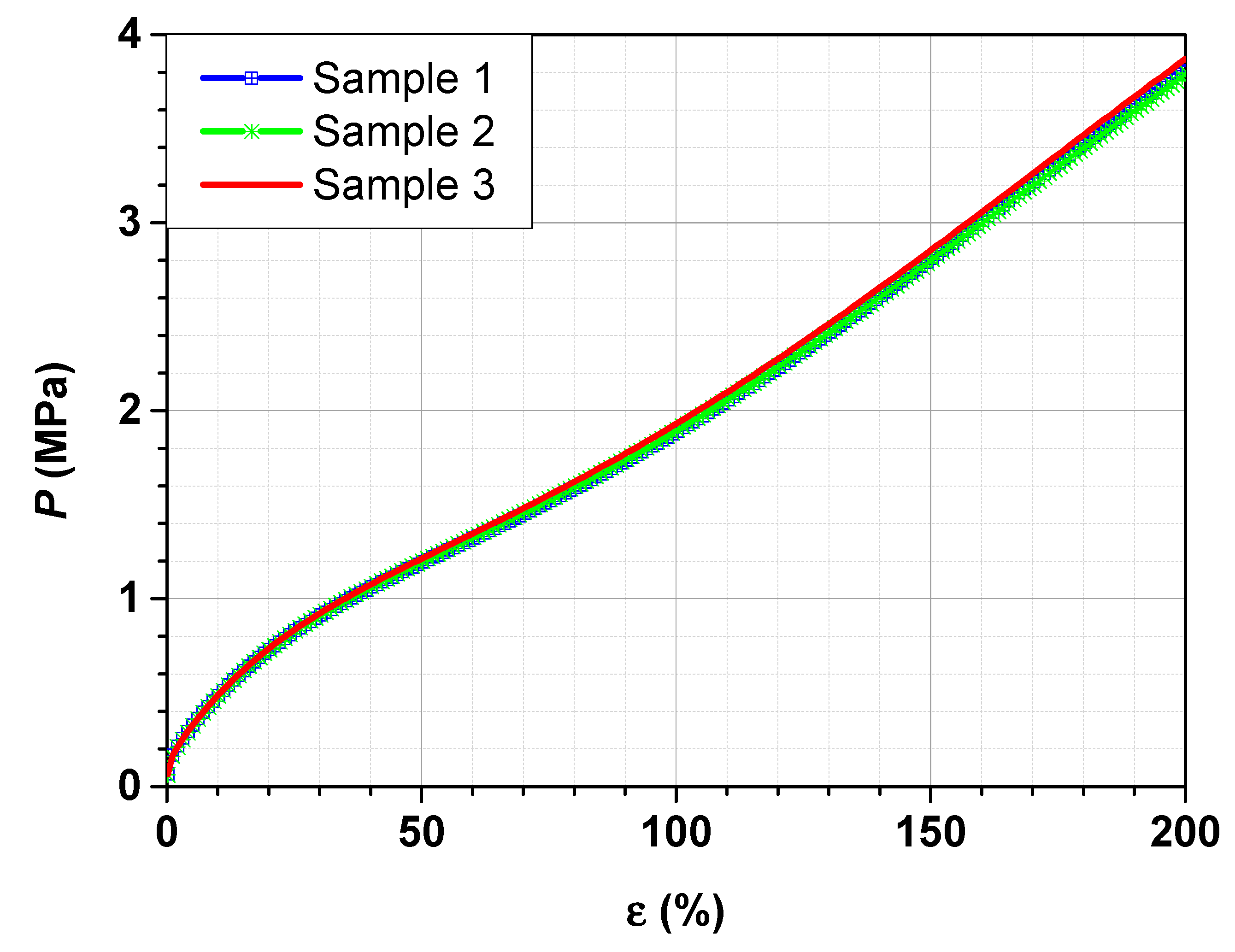
The stress–strain curves for the SBR filled with 70 phr carbon black N234 measured in tensile are shown in Figure 3.

Figure 3 shows three stress–strain curves suggesting an excellent reproducibility of the measurement data with a slightly small statistical deviation, due to material inhomogeneity. One representative stress–strain curve of the SBR sample filled with 70 phr N 234 is fitted with Abaqus using the neo-Hooke (NH), Mooney–Rivlin (MR) and Yeoh (Y) models. The respective fit curves are shown in Figure 4.

The curve fitting shows different course along the measured stress–strain curve. Compared to the neo-Hooke and Mooney–Rivlin models, the Yeoh model matches the most suitable curvature of the stress–strain curves for SBR samples filled with 70 phr N234 in tensile.

The mean squared error was used as a criterion for the fitting quality of the three hyperelastic material models. The smaller the mean squared error, the better the fitting quality. The determined mean squared error of the fit curves and the measurement curve in tensile are listed in

Table 2. Mean squared error of the measurement curve in tensile and the fit curves using neo-Hooke, Mooney–Rivlin and Yeoh models.

	Neo-Hooke	Mooney–Rivlin	Yeoh
Mean squared error	0.027	0.017	0.006

.

The Yeoh model provides the smallest mean squared error and thus provides the best fit. The neo-Hooke comes off the worst.

This step aims to determine according to Equations (19), (21) and (23) the material constants $C_1$, $C_2$ and $C_3$. The obtained fit parameters are summarized in

Table 3. Fit parameters of a stress–strain curve of the SBR filled with 70 phr N234 using neo-Hookean, Mooney–Rivlin and Yeoh models.

	${\mathit{C}}_1$ [MPa]	${\mathit{C}}_2$ [MPa]	${\mathit{C}}_3$ [MPa]
Neo-Hooke	0.6002	-	-
Mooney–Rivlin	0.7216	−0.2837	-
Yeoh	0.5621	−0.0052	0.0014

.

The material constants $C_1$, $C_2$ and $C_3$ are used to calculate the strain energy density function $W$ according to Equations (18), (20) and (22) for neo-Hooke, Mooney–Rivlin and Yeoh materials respectively. The strain energy density function $W$ as a function of the principal stretch ratio $\lambda$ for the uniaxial tension and compression deformation state is plotted in Figure 5.

In Figure 5, the characterized principal stretch ratio $\lambda =1$ represents the state without deformation because this implies a zero-strain $\epsilon = 0$ according to Equation (11). Above this limit, the SBR sample is subjected to a uniaxial tensile strain. Below this limit, the SBR sample is subjected to a compression deformation. In real applications, rubber samples can be compressed up to $50\%$ corresponding to a principal stretch ratio of $\lambda =0.5$. As an incompressible material, the principal stretch ratio $\lambda =0$ is for rubber out of reach.

The strain energy density functions $W$, calculated as a function of the principal stretch ratio $\lambda$ from the fit parameters obtained in Table 1 using the neo-Hooke, Mooney–Rivlin and Yeoh models, show a quite similar curve shape for the tensile area. The deviations become obvious between the single curves at high loads even though the general trend remains preserved. For the compression area, the Mooney–Rivlin curve deviates already at small strains from the tighter neo-Hooke and Yeoh curves.

In the following, the Yeoh graph is discussed in detail. The conclusions obtained are also valid for the Mooney–Rivlin and neo-Hooke graphs. Only the numerical values vary. The principal stretch ratio $\lambda = 0.8$ corresponds to a compression deformation of $20\%$. The corresponding strain energy density function $W$ is $0.08$ MPa. The same $W$ can also be assigned to the principal stretch ratio $\lambda = 1.23$. This means, for the same strain energy density function $W$, the SBR sample can also be stretched to a deformation of $23\%$ instead of the compression deformation discussed above. Additional two strain energy density functions $W$ are selected: $0.04$ MPa and $0.16$ MPa.

The selected strain energy values cover a wide load range for real applications. Up to 30% compression deformation represents a typical load during applications for rubber materials like seals or tires.

The correlated strains in the uniaxial tension and compression are determined for the three models used and are summarized in

Table 4. Determination of the compression-equivalent strain of SBR measured in tensile mode from the strain energy density function $W$ calculated using the neo-Hooke, Mooney–Rivlin and Yeoh models.

	Strain Energy Density Function W [MPa]	Compression Strain [%]	Tensile Strain [%]
Neo-Hooke	0.04	−14.5	16.0
	0.08	−20.0	23.0
	0.16	−27.5	33.0
Mooney–Rivlin	0.04	−16.0	17.0
	0.08	−23.0	24.2
	0.16	−32.0	35.0
Yeoh	0.04	−14.5	16.0
	0.08	−20.0	23.0
	0.16	−27.5	34.0

.

It can rightly be claimed that for the same strain energy density function $W$, independently of the hyperelastic model used, the sample can be either stretched or compressed depending on the deformation direction. It should be noted, that due to the incompressibility constraint of rubber the absolute value of the attained strain in tensile is always larger than that in compression.

To check these findings, three stress–strain curves in compression mode for SBR filled with 70 phr carbon black N234 are performed. The test results are shown in Figure 6.

Similar to stress–strain measurement in tensile, Figure 6 confirms an excellent reproducibility of the measurement. A small statistical deviation is however inevitable due to material inhomogeneity.

Figure 7 illustrates a representative stress–strain curve of the SBR sample in compression mode and the corresponding simulated curves using the neo-Hooke, Mooney–Rivlin and Yeoh models derived from measurement data in tensile.

Compared to tensile measurements, the simulated stress–strain curves in compression mode using the Mooney–Rivlin model differs considerably from the results obtained using the neo-Hooke and Yeoh models, which are almost comparable.

The simulated stress–strain curve for compression differs quite clear from the experimental measurement in contrast to tensile results, even for the Yeoh model, which fits the measurement results performed in tensile.

The determined mean-squared errors of the fit and the measurement curves in compression are listed in

Table 5. Mean squared error of the measurement curve in compression and the fit curves using neo-Hooke, Mooney–Rivlin and Yeoh models.

	Neo-Hooke	Mooney–Rivlin	Yeoh
Mean sqaured error	0.0332	0.300	0.0501

.

The best fit quality is achieved with the neo-Hoke model. The Mooney–Rivlin model provides the poor fit quality. The fit quality of the Yeoh model is comparable to the neo-Hooke model.

The measured stress–strain curve is significantly stiffer than the three simulated curves. This behavior is due to the assumption made for the boundary conditions in the simulation. For the uniaxial compression, a homogeneous deformation state is assumed; neglecting the edge effects and friction between the sample and the sample holder.

From the raw data of the compression test, the area above the corresponding stress–strain curve represents the strain energy density function $W$.

$W$ calculated from the raw data for compression and tensile tests as well as the standard deviation are shown in

Table 6. Strain energy density function $W$ calculated from the raw data for compression and tensile tests.

	Tensile Strain [%]	Compression Strain [%]	$\mathit{W}$ from Tensile [MPa]	$\mathit{W}$ from Compression [MPa]	Deviation [%]
Neo-Hooke	16.0	−14.5	0.066	0.073	−9.59
	23.0	−20.0	0.116	0.126	−7.94
	33.0	−27.5	0.204	0.225	−9.33
Mooney–Rivlin	17.0	−16.0	0.072	0.085	−15.29
	24.2	−23.0	0.124	0.161	−22.98
	35.0	−32.0	0.223	0.296	−24.66
Yeoh	16.0	−14.5	0.066	0.073	−9.59
	23.0	−20.0	0.116	0.126	−7.94
	34.0	−27.5	0.213	0.225	−5.33

.

The material models neo-Hooke and Yeoh show a deviation below 10% between the measured and simulated strain energy density function $W$ for all strain amplitudes. The Yeoh model even shows a reduced deviation with increasing strain amplitudes. The deviation of the simulated value for compression at 27.5% is only about 5%. This behavior is due to a better match of the stress–strain curves for SBR samples filled with 70 phr N234 in tensile.

These results are within the simulation inaccuracies related to the simple assumptions made-no edge effects and no friction between the sample and the sample holder-and are in line with our expectations. It is worthy to note, that the deviation between the measured and simulated strain energy density function $W$ using the Yeoh model decreases with increasing the strain.

The Mooney–Rivlin model delivers a deviation between the measured and the simulated strain energy density function $W$ larger than 15%. These unsatisfactory results are already guessed due to the poor fit quality compared to neo-Hooke and Yeoh models, observed in Figure 7.

5. Conclusions

The aim of this study is to simulate from experimental data measured in tensile how the stress–strain curves in compression mode look like and subsequently to compare them with real test results.

The way to match the tensile and compression modes together is based on hyperelastic models for rubber materials. First, neo-Hooke, Mooney–Rivlin and Yeoh models are used to fit experimental data measured in tensile. From that, the strain energy density function $W$ is calculated and then extrapolated to compression mode. The first Piola–Kirchhoff stress, and thus a “simulated” stress–strain curve in compression mode are derived.

The simulations show taking into account the degree of simplicity of the material models used as well as non-consideration of friction and the edge effects a good agreement to the result measured in compression mode. It is true, none of the implemented models exactly captures the real behavior of the SBR material in compression. However, the deviation remains smaller than 10% for the neo-Hooke and Yeoh models. The deviation even decreases with increasing the strain using the Yeoh model implying a better capture of the measurement results at large displacements. This makes the Yeoh model more appropriate than neo-Hooke and Mooney–Rivlin models to describe the large non-linear behavior of rubber materials. With a deviation of up to 25%, the Mooney–Rivlin model is performing poorly in comparison to neo-Hooke and Yeoh models.

The relationship achieved between the strain amplitudes in tensile and compression tests using Yeoh and neo-Hooke material models provides better adjustment curves to measurement results compared to Mooney–Rivlin material model.

Mooney–Rivlin overestimates the strain amplitudes in compression due to the poor prediction of the stress–strain curve in compression from experimental results.

Therefore, a good relationship between the tensile and compression modes is established. This serves to save time and money. For this purpose, the neo-Hooke model would be enough.