Article

Automated Thoracolumbar Stump Rib Detection and Analysis in a Large CT Cohort

1
Department for Interventional and Diagnostic Neuroradiology, TUM University Hospital, Ismaninger Straße 22, 81675 Munich, Germany
2
Chair for AI in Healthcare and Medicine, Technical University of Munich (TUM) and TUM University Hospital, 81675 Munich, Germany
3
Department of Radiology, Weill Cornell Medicine, 1300 York Ave, New York, NY 10065, USA
4
Department of Radiology, TUM University Hospital, Ismaninger Straße 22, 81675 Munich, Germany
5
German Cancer Consortium (DKTK), Munich Partner Site, 69120 Heidelberg, Germany
6
Department of Diagnostic and Interventional Radiology and Nuclear Medicine, University Medical Center Hamburg-Eppendorf, 20251 Hamburg, Germany
7
Department of Quantitative Biomedicine, University of Zurich, Winterthurerstrasse 190, 8057 Zurich, Switzerland
8
Department of Computing, Imperial College London, 180 Queen’s Gate, London SW72AZ, UK
9
Department of Diagnostic and Interventional Radiology, University Medical Center Rostock, Schillingallee 35, 18057 Rostock, Germany
*
Author to whom correspondence should be addressed.
AI 2026, 7(6), 224; https://doi.org/10.3390/ai7060224
Submission received: 12 May 2026 / Revised: 9 June 2026 / Accepted: 10 June 2026 / Published: 16 June 2026
(This article belongs to the Section Medical & Healthcare AI)

Abstract

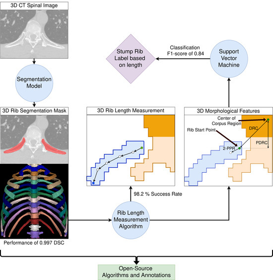
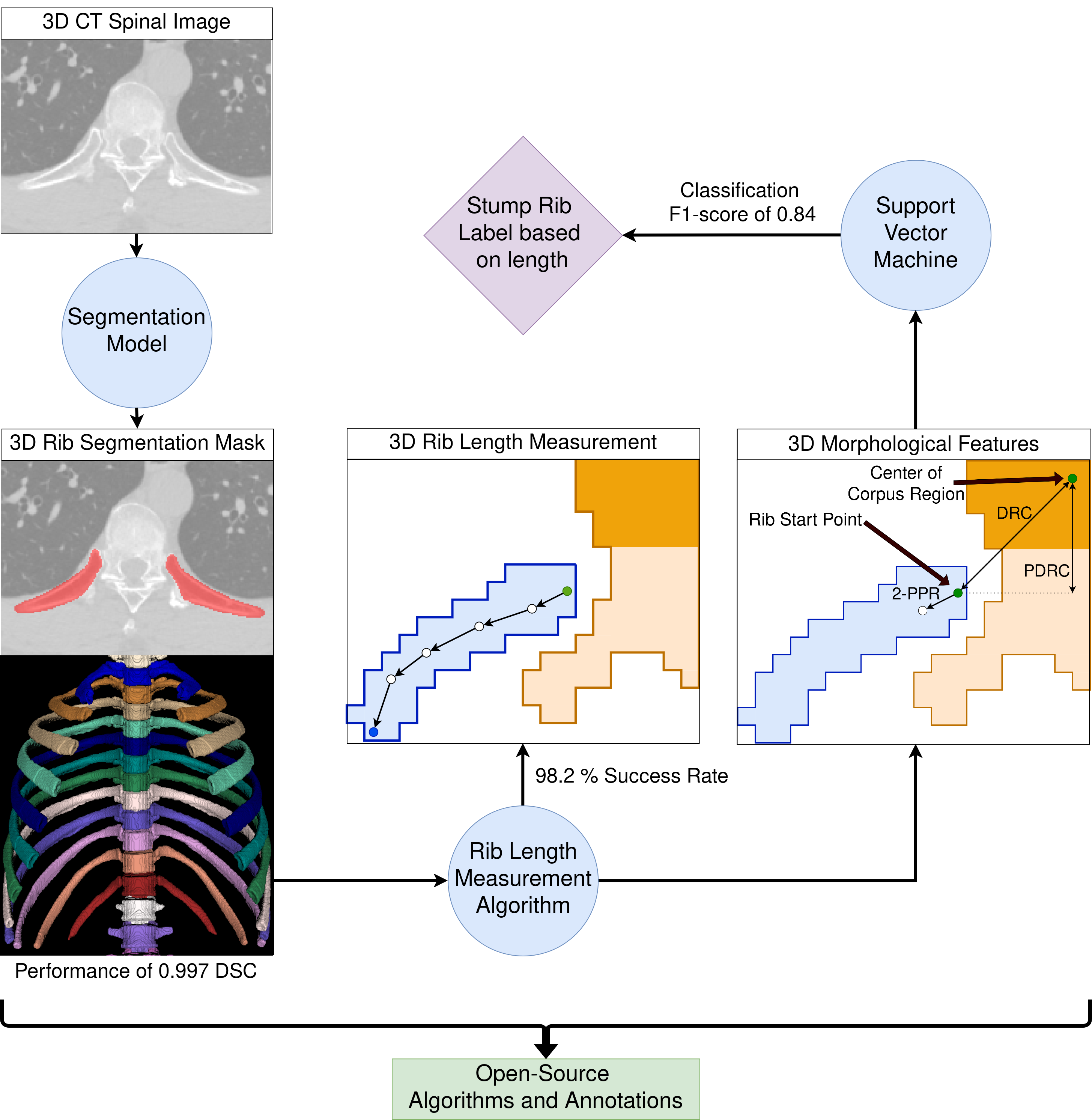
Thoracolumbar stump ribs are one of the essential indicators of thoracolumbar transitional vertebrae or enumeration anomalies. While some studies manually assess these anomalies and describe the ribs qualitatively, this study aims to automate thoracolumbar stump rib detection and analyze their morphology quantitatively. To this end, we train a high-resolution deep learning model for rib segmentation using nnUNet and achieve significant improvements over existing models (Dice score 0.997 vs. 0.779, p-value < 0.01). In addition, we employ a novel iterative algorithm and piecewise linear interpolation to estimate rib length, achieving a success rate of 98.2%. When analyzing morphological features, we show that stump ribs articulate more posteriorly at the vertebrae ( 19.2 ± 3.8 vs. 13.8 ± 2.5 mm, p-value < 0.01), are thinner ( 260.6 ± 103.4 vs. 563.6 ± 127.1 mm 2 , p-value < 0.01), and are oriented more downwards and sideways within the first centimeters in contrast to full-length ribs. We show that with partially visible ribs, these features can achieve an F1-score of 0.84 and an AUC of 0.98 in differentiating stump ribs from regular ones. We publish the model weights and masks for public use.

Graphical Abstract

1. Introduction

The human spine typically consists of 24 presacral vertebrae, of which seven are cervical, twelve are rib-bearing thoracic, and five are lumbar vertebrae [1]. Nevertheless, the number of vertebrae may vary, leading to thoracolumbar transitional vertebrae (TLTV). TLTV is defined as a vertebra that has partial features of thoracic as well as lumbar vertebrae and has a dysplastic/hypoplastic rib [2,3]. These so-called stump ribs, by common definition, have a length of 38 mm and can only appear at the lowest thoracic level [3]. Moreover, Tatara et al. [2] found additional indicators for TLTV, such as anomalies in rib shape. This can occur, for example, due to a deformation of the rib head. The thoracolumbar junction is considered a weak connection, so injuries, such as fractures or thoracolumbar junction syndrome, often occur here [4,5]. These biomechanical changes might be crucial for surgical planning, as they can affect surgical outcomes and recovery [6,7]. Additionally, the occurrence of TLTV often indicates numerical anomalies, such as an additional or missing thoracic vertebra.
Overall, detecting such anomalies is vital for accurate assessment of vertebral heights and for localizing weak points. Automating this process would reduce radiologists’ work and increase the accuracy of surgical planning. Moreover, some CT reformations are not wide enough to capture the whole extent of the ribs. In these cases, a manual assessment of thoracolumbar stump ribs is so far infeasible. We aim to automatically localize and detect stump ribs and exploit rib-shape differences between stump ribs and regular ribs to detect stump ribs even with partially visible ribs.
For this to work, we need to automatically localize ribs in a CT image, measure their lengths, and extract morphological features. We opt to address this by creating dense, complete segmentation masks. Segmentation is the task of assigning a label to each pixel of an input image [8]. In our case, the input images are CT images, and we want to assign each voxel to a rib structure. We then calculate the lengths of the ribs and other morphological features from these segmentations. After that, we can compare stump ribs and regular ribs based on these features and use them to differentiate the two groups without using length.
For developing solutions to automate the creation of segmentation annotations, deep learning has become a prominent field in science. Specifically, segmentation has been used in the past to localize and describe medical structures [9], and it is considered state-of-the-art. Previously, most existing approaches to ribs used segmentation or center-extraction algorithms [10,11,12,13,14,15,16,17], which are not publicly available. The TotalSegmentator [18] is publicly available and can segment ribs, yet it is unable to yield a quality sufficient for rib-length calculations. We expand the rib segmentation to capture the entire rib, develop a length-measurement algorithm, and make our model and segmentation masks available, thereby bridging a gap in the community. Finally, to the best of our knowledge, no work has attempted to automate stump rib detection or to conduct quantitative experiments contrasting regular ribs with stump ribs using automated morphological features.
The contributions of this study are:
  • We develop a whole rib segmentation tool for CT imaging and present a rib length measurement algorithm based on that segmentation.
  • We automatically detect and localize thoracolumbar stump ribs by calculating the rib length.
  • We describe stump rib morphological features in contrast to regular ribs and propose them as additional indicators of stump rib occurrence.
  • We show that these morphological features classify stump ribs even with a partial field of view.
  • We make the segmentation model, assessment algorithm, and manual and predicted rib segmentation masks publicly available (https://github.com/Hendrik-code/rib-segmentation, accessed on 2 March 2026).

2. Materials and Methods

2.1. Data

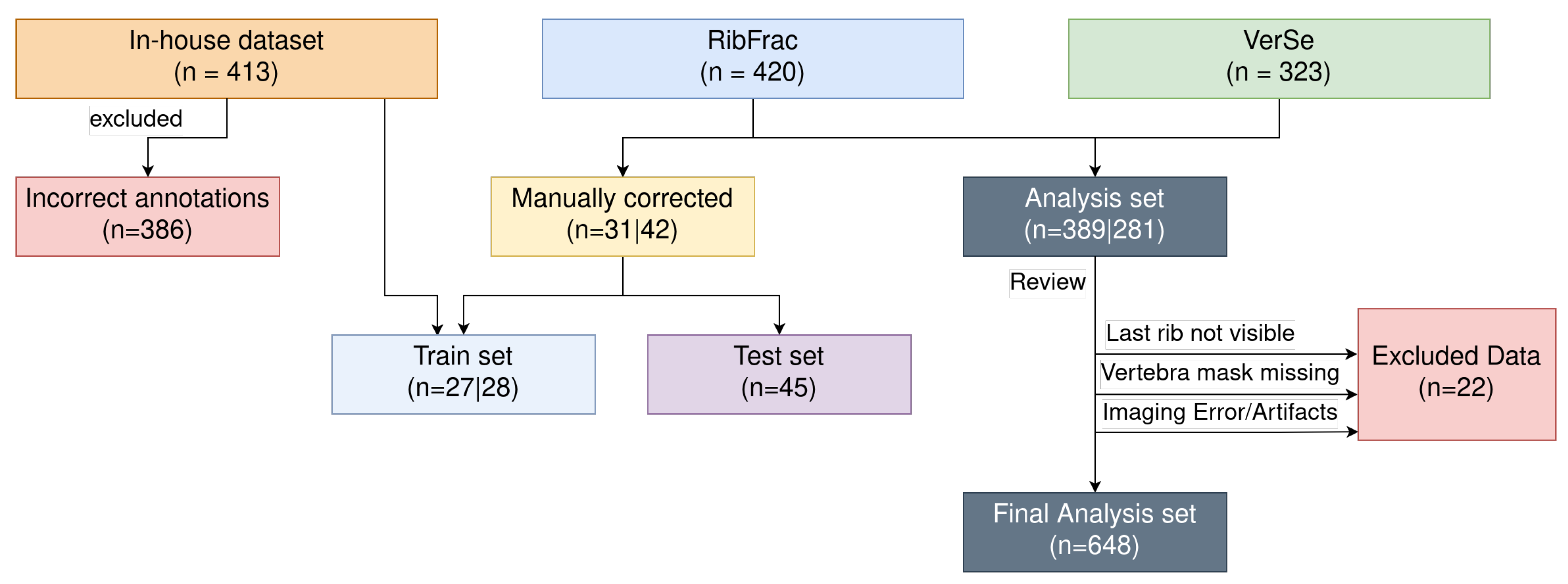
This study used three CT datasets (see Figure 1). Two publicly available ones, VerSe [19] and RibFrac [20,21], and a private in-house dataset. For demographics, see Table 1. The VerSe data has expert-quality vertebra segmentation annotations. Thanks to Jin et al. [22], the RibFrac data includes instance segmentations of the ribs (called RibSeg). The in-house dataset contains binary annotations of ribs created by one expert, A.D., separating rib tissue from background.

2.2. Segmentation Approach

To measure the length of the ribs, we require dense and complete segmentation annotations. We define a correct rib annotation as the filled bone outline (indicated by high-intensity values in CT) up to, but not including, the costal cartilage and the sternum.
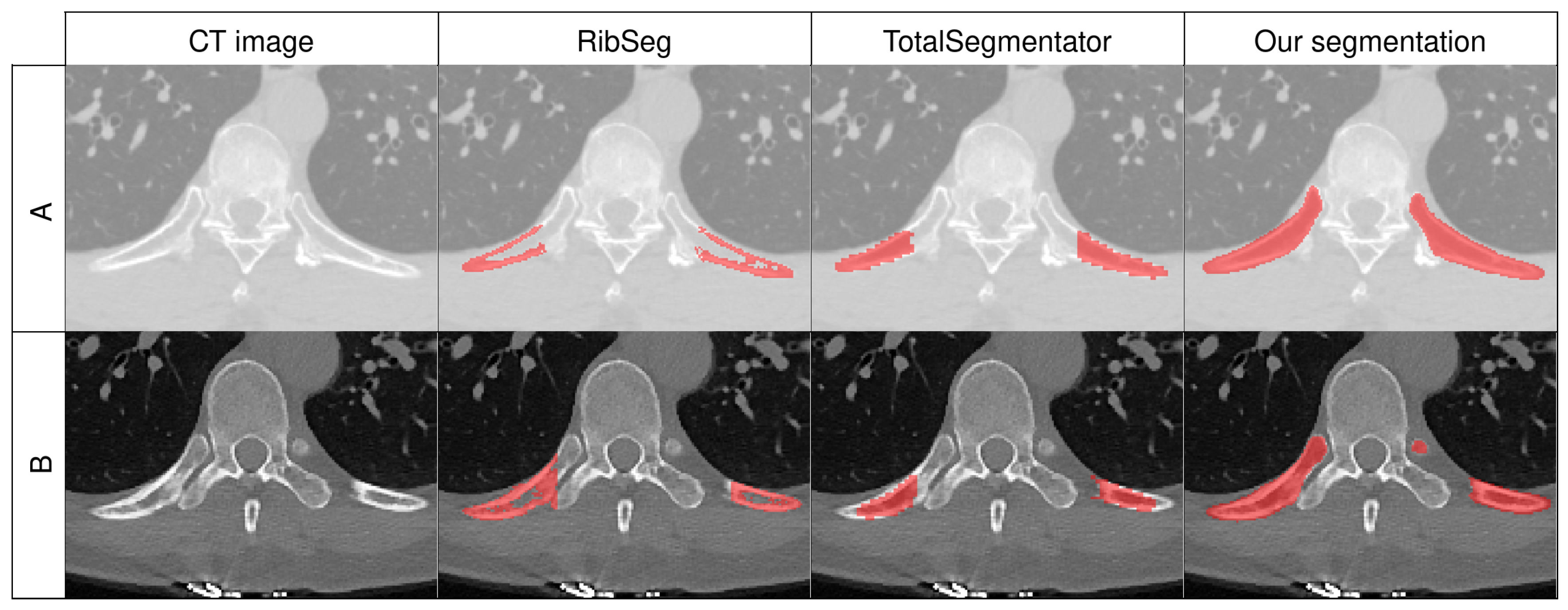
We observed that the rib annotations in the RibFrac dataset exclude the rib heads. The TotalSegmentator [18] exhibits the same issue (see Figure 2). Thus, we developed our own rib segmentation model by utilizing nnUNet [9], a widely used architecture for training semantic segmentation models. We started with a small set of annotations from the in-house data, ran inference on public datasets, manually corrected some to expand the training set, and then trained again.
In detail, we used 27 subjects from the in-house data with high segmentation quality (see Figure 1). We trained a default nnUNet 3d fullres configuration with the suggested parameters, except for the patch size, which we set to a consistent cubic size of 192 × 192 × 192. We trained for 300 epochs with 3-fold cross-validation, resampling the training data to a consistent isotropic resolution of 0.8 mm. This value of 0.8 mm was chosen as a compromise between accuracy and computational feasibility, not a tuned hyperparameter. Additionally, we used elastic deformation (parameters chosen qualitatively) and random horizontal flipping to augment our data by a factor of ten.
We then applied this model to the public datasets. After careful review, we chose 17 subjects from VerSe and 11 from RibFrac. These annotations, along with another 45 randomly selected subjects from VerSe and RibFrac, were manually corrected by an expert (H.M.) with two years of experience. Two experts (H.S., J.S.K.), with three and 23 years of experience, respectively, supervised the corrections and reviewed them to ensure quality. We used ITKSnap 3.8.0 [23] for annotation review and manual correction in all three dimensions. The 45 randomly selected subjects were used exclusively as the test set. The resulting training split, totaling 55 subjects, was used to retrain the rib segmentation model using the same training procedure.
Figure 2 compares our rib segmentation tool to existing approaches. These rib annotations are binary and thus only distinguish between foreground (ribs) and background (not ribs). The created manual and predicted segmentation masks from this study are published under https://doi.org/10.5281/zenodo.14850928.

2.3. Instance Assignment

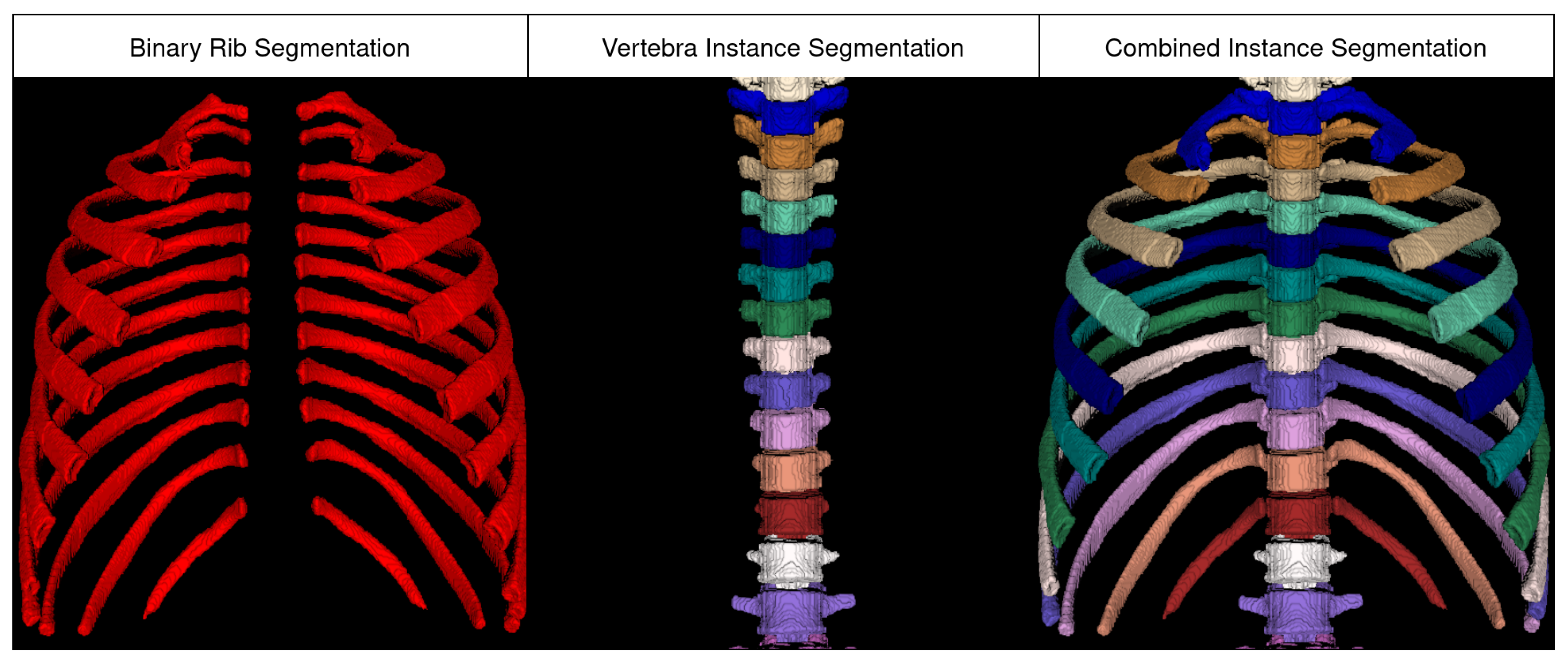
Our goal is to derive information for each rib individually. This requires instance segmentation masks of the ribs, not only semantic ones. To bridge this gap, we used vertebra instance segmentation masks. The VerSe data already contained expert-level annotations for individual vertebrae. We used the Bonescreen SpineR tool (Bonescreen GmbH, Munich, Germany) based on Sekuboyina et al. [24] to generate vertebra segmentations for the RibFrac dataset. We then derived the connected components from the predicted binary rib segmentation mask of our model and assigned the rib components to the vertebrae based on spatial proximity. To ensure robust results, we employed the constraints that each vertebra can only have two ribs, and each rib can only be assigned to one vertebra (see Figure 3). Moreover, we distinguished the side of the rib by comparing the rib localization to its corresponding vertebra. We encountered instances where a rib was segmented, but its corresponding vertebrae had not been segmented. In these cases, we consistently relabeled these rib instances to a set of unused labels. We manually reviewed the subjects using the generated 2D coronal and sagittal snapshots.

2.4. Rib Length Measurement

Now that we can localize and view each rib in our images individually, we need to measure the length of a single rib to assess whether it is a stump rib (SR). For that, we employed an iterative algorithm to calculate points along a path. We started by cropping a single rib combined with its corresponding vertebra. To ensure consistency, we rescaled the cropped segmentation mask to a fixed resolution of 0.5 mm for each dimension. The 0.5 was chosen based on initial observations. A higher resolution leads to computational infeasibility, while a lower resolution quickly exhibits larger interpolation errors due to the inherent discreteness of voxels. We filled 3D holes to ensure the segmentation remained dense while maintaining the overall shape and size.
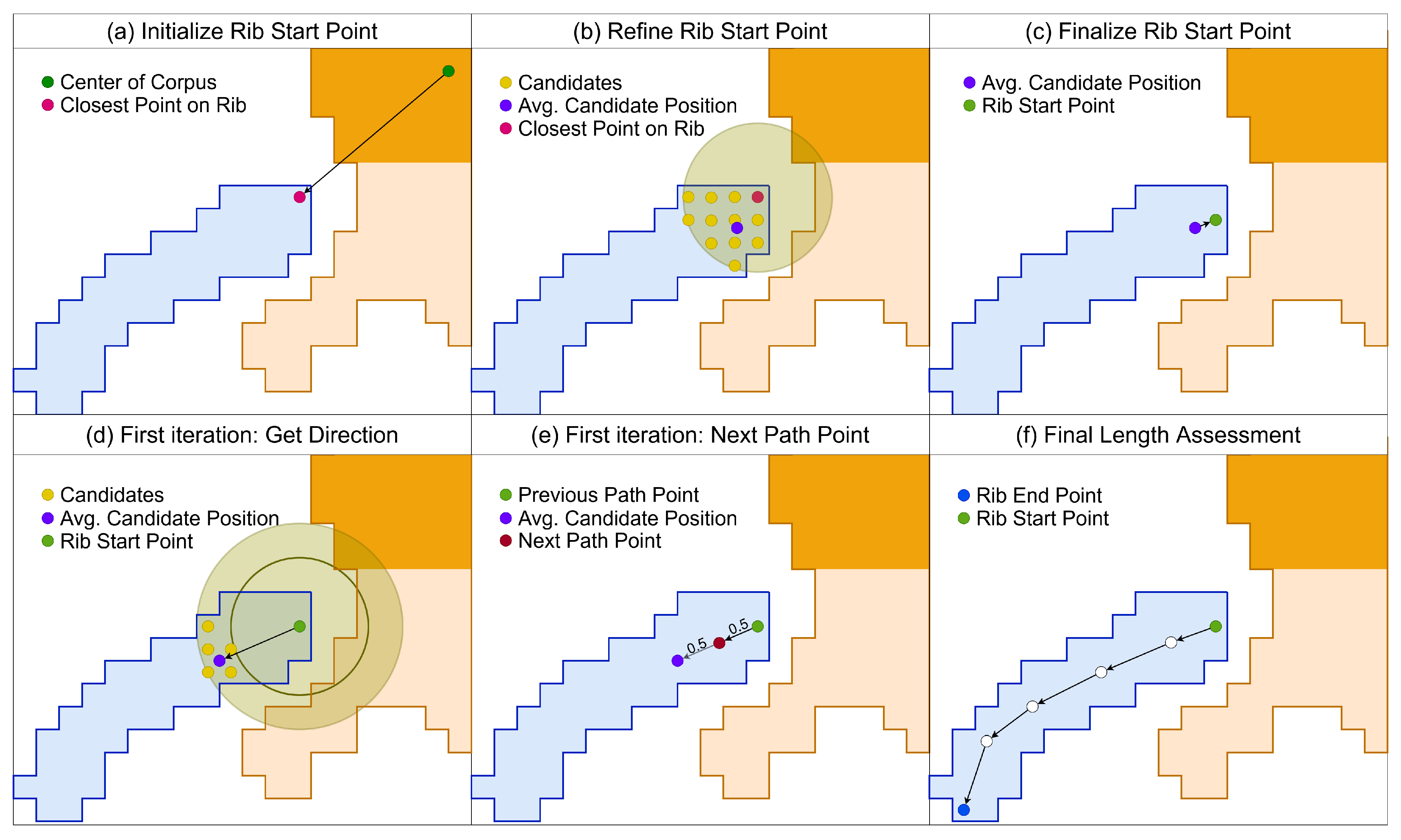
The rib-length measuring algorithm (RLMA) starts by locating the rib’s start point. We select the closest point on the segmentation surface to the center of mass of the corresponding vertebra corpus. We refine the location by averaging all surrounding segmented voxels and projecting the result onto the segmentation surface (see Figure 4). This ensures the start position is already at the middle of the rib, not at a corner. We set this start point as the first path point.
From the start point, we iteratively add path points along the center of the rib. For this, we find all candidate points within a circular distance of 14.5 to 15.5 mm from the previous path point. We remove all candidate points in that list that are closer to any prior path point than the latest, ensuring that we are iterating in the correct direction. We then take the average coordinate location of all these candidate points. We can compute a direction vector in relation to our previous path point. Moving from the latest point halfway along that direction vector gives us our next target. This new location gets projected onto the nearest segmentation voxel and is added as the next path point (see Figure 4). This gets repeated until we reach the end of the rib, where no possible points lie on the circular slice. To find the final path point, we shoot a cone of ray-casts from the latest path point along the vector of the previous path point and find the point in those ray-casts that is furthest away from the latest path point. We take this as the endpoint. To calculate the length, we take the path points and sum the distances between them.
The circular distance range of 14.5 to 15.5 mm was chosen to accommodate the 0.5 mm resolution. It is a straight 30-voxel distance at that resolution, with some flexibility to allow for diagonal distances. This parameter was chosen based on initial observations: much lower and much higher values reduced the algorithm’s stability (very close path points produce jittery paths, while larger distances reduce accuracy).
By definition, thoracolumbar stump ribs (SR) are shorter than or equal to 38 mm [3]. We compare this threshold to the length computed by our RLMA. This yields a binary label (SR or not-SR) for each rib.

2.5. Morphological Features

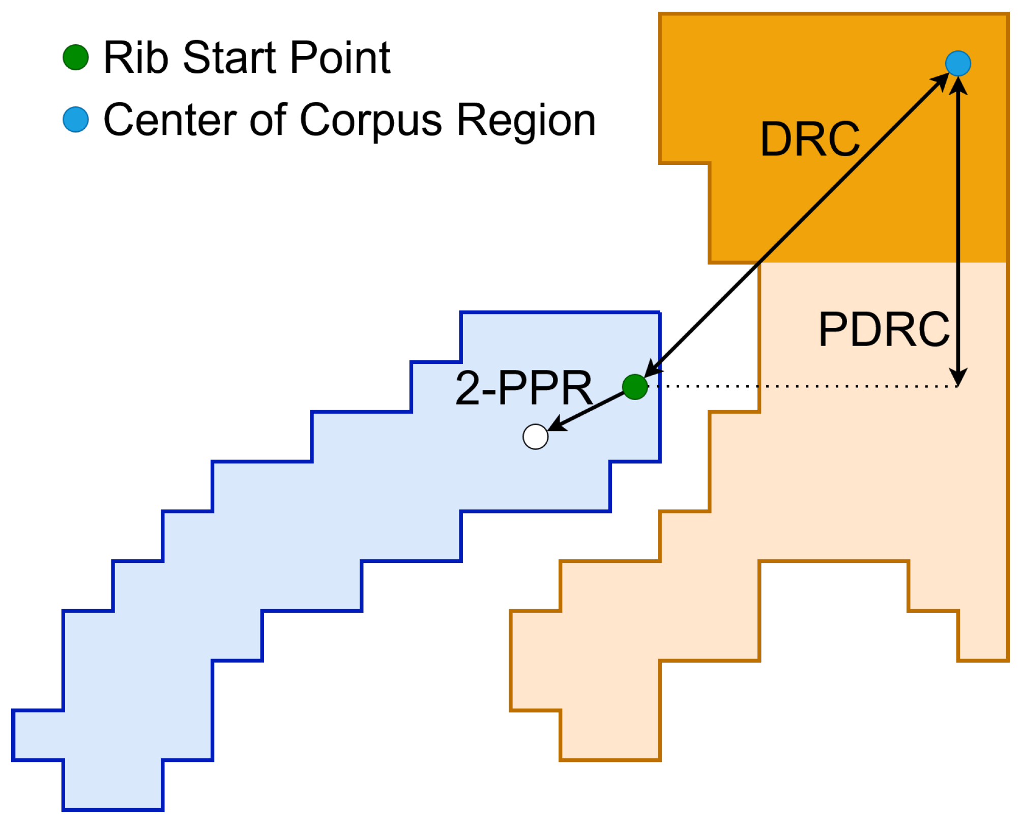
We calculate morphological features from our rib segmentations. We compute the spatial relation vector between the rib’s start point and the corresponding vertebra corpus center (DRC). Specifically, we examine the posterior distance between the rib and the corpus center, which we denote PDRC (see Figure 5). Additionally, we use the path points and their spatial relationships via the direction vectors between neighboring path points. We denote n-PPR as the spatial relation vector for the first n path points. For example, 2-PPR means the direction vector from the rib’s start point to its next path point. From the RLMA, we have the rib’s length; using the segmentation mask, we can calculate the volume-to-length ratio.
To account for rotation, we use the orientation of each vertebra and multiply the inverted rotation matrix by the measured features to obtain rotations relative to each vertebra. Additionally, to be consistent, we mirror the left ribs onto the right side. This means that the right dimension always points away from the vertebra.

2.6. Experiments

We utilized the two public datasets (VerSe and RibFrac) for all downstream experiments. We ran our rib segmentation across all subjects and the rib-length measuring algorithm (RLMA) on the lowest two vertebrae with ribs present.
We compare the segmentation performance on our manually corrected test set. Our baselines are the RibSeg segmentation masks (both with and without fill holes applied) and the TotalSegmentator. We evaluate this on various metrics (see Appendix A). This yields a comparative analysis regarding the segmentation performance.
For the rib length analysis, we used the analysis set (all subjects from VerSe and RibFrac that are not in the training set) and incorporated some exclusion criteria: We excluded 36 subjects in which the last rib is not visible in the image, 78 ribs for which the corresponding vertebra segmentation was missing, and two subjects with imaging artifacts (see Figure 1 for detailed data flow).
Then, two experts (H.S., B.K.) reviewed the generated ribs segmentation for segmentation and measurement errors. As there is no standard in manually measuring the rib length, the experts categorized each rib into a five-point Likert scale: (1) the segmentation has major errors or segmented the wrong structure, (2) the segmentation is the correct structure but erroneous enough so that the resulting length is wrong, (3) the segmentation touches the border of the image and thus the length of the visible section is correct but incomplete, (4) the segmentation has minor mistakes which did not impact the length calculation, and (5) everything is fine. The relative frequency of this rating indicates how often our segmentation, combined with our RLMA, successfully measured rib length.
For the morphological analysis, we included ribs with certainty about their SR label. Hence, we only used ribs marked with (4) and (5) and those with (3) where the length of the visible part already exceeded the SR threshold.
We show how well we can separate stump ribs from regular ribs using morphological relations to the corresponding vertebra without using the full length of the ribs. Thus, we use the DRC features as input for a Support Vector Machine (SVM) [25] to differentiate stump ribs and regular ribs. We also used n-PPR as input features for the SVM. We test this with n set to 2, 3, and 4 to see how much of a rib needs to be visible to predict stump ribs. Going beyond n = 4 would yield a measured length close to or beyond the SR threshold, thereby defeating the purpose. We also combine n-PPR and DRC as input features to see whether this improves the performance.
For all SVM experiments, we repeat the setup with 10 different fixed seeds and a random 70/30 train/test subject-wise split to assess a robust separability performance. We report the F1, balanced accuracy, and AUC scores averaged over the 10 runs. Additionally, we compare this setup to logistic regression (LoRe) and multilayer perceptron (MLP). We did not address class imbalance for this, other than ensuring approximately equal numbers of SR cases across splits. Input features were always normalized based on the mean and standard deviation across the training samples of a split.
Finally, we perform a robustness analysis of the RLMA on the manually corrected test set. We compare the measured rib length in the reference annotations with that in the predicted annotations (see Appendix C).

2.7. Statistical Analysis

To compare the statistical significance of our segmentation models, we use the Wilcoxon signed-rank test [26] on Dice scores, with p < 0.05 indicating statistical significance. For the feature distributions grouped by stump ribs and regular ribs, we perform the Wilcoxon rank-sum test and use the same threshold for statistical significance.

2.8. Software

To conduct this study, we used Python v3.11, TPTBox v0.4.2, panoptica v1.1.4, and nnUNetv2 v2.6.2. All statistical significance tests were computed using SciPy v1.14.1.

2.9. Hardware

The nnUnet segmentation model was trained on an NVIDIA A40 GPU for approximately 30 h. The CPU used was an AMD EPYC 7413 with more than 100 GB of available RAM.

3. Results

3.1. Segmentation Performance

Our model trained on 55 samples outperforms the TotalSegmentator on 45 randomly selected, manually corrected test subjects (see Table 2). We hypothesize that this is primarily due to the TotalSegmentator’s inability to segment the rib heads and its inferior segmentation resolution.
The public RibSeg annotations [22] for the RibFrac dataset are also inferior compared to our rib segmentation model (see Table 3). Our model consistently outperforms on every metric and sample with a significant margin (p-value < 0.01 ).

3.2. Rib Length Measurement

Based on the manual review of our experts, 98.2% of the lowest two ribs in both public data sets were correctly segmented and measured (see Table 4), thus yielding a correct stump rib assessment. Only in 1.8% of the cases did we have segmentation errors that influenced the rib length measurement. After a manual review of these cases, there was only one rib with a measured length close to the stump rib threshold of 38 mm. We observed that the length calculation is only slightly erroneous in all other cases. Thus, we can confidently state that the errors in rib length calculation for all but one of these cases would not have influenced their stump rib label. For a qualitative analysis of the observed errors, see Appendix B. A quantitative analysis of how the segmentation model’s prediction errors influence the measured rib length is shown in Appendix C.

3.3. Morphological Features

After our exclusions, we ended up with 2464 individual ribs across 648 subjects, all of which were the subject’s lowest or second-lowest rib. We did not observe any bias in our exclusion criteria, such as pathologies or anomalous intensities. Of the 2464 ribs that we analyzed, 159 were stump ribs. Of the 648 subjects, 133 had at least one SR (20.5%), according to the 38mm length threshold for stump ribs.
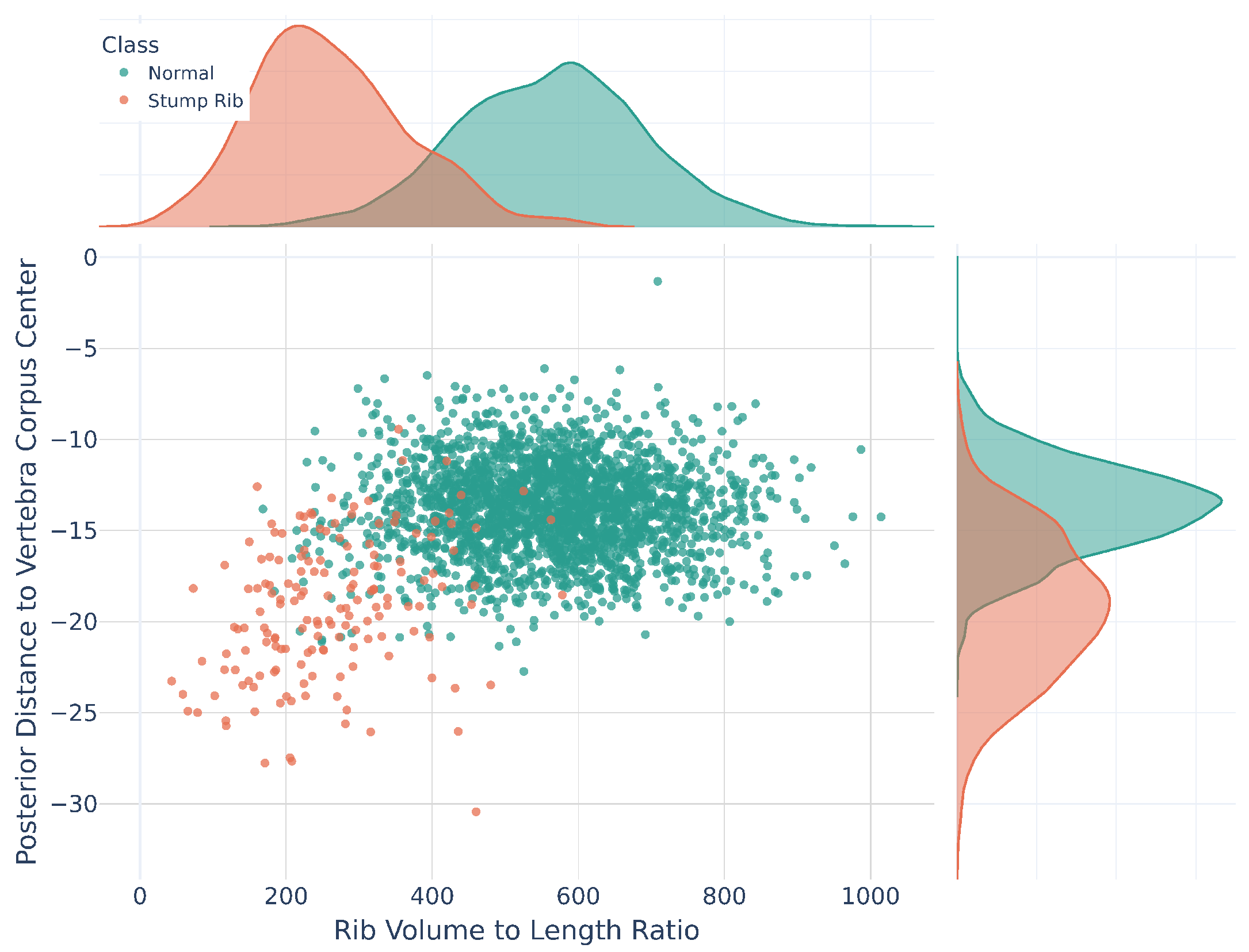
On average, the distance in the posterior direction between the corresponding vertebra corpus center and the closest point on the rib was increased for stump ribs ( 19.2 ± 3.8 vs. 13.8 ± 2.5 mm, p-value < 0.01), and they had a lower volume-to-length ratio ( 260.6 ± 103.4 vs. 563.6 ± 127.1 mm 2 , p-value < 0.01, see Figure 6).
We manually inspected the samples with a high posterior distance to the corresponding corpus, but they were not classified as stump ribs based on their length. Here, we observed that most samples’ vertebrae had an enlarged fovea pushing the rib’s beginning posteriorly, or an anomaly in the corpus region, shifting the corpus center to an unnatural position. This indicates that the higher posterior distance is not due to the morphology of the rib but rather to that of the vertebra. Thus, we hypothesize that accounting for vertebra morphology should further enhance the separability between SR and regular ribs by using the posterior vertebra distance relation.
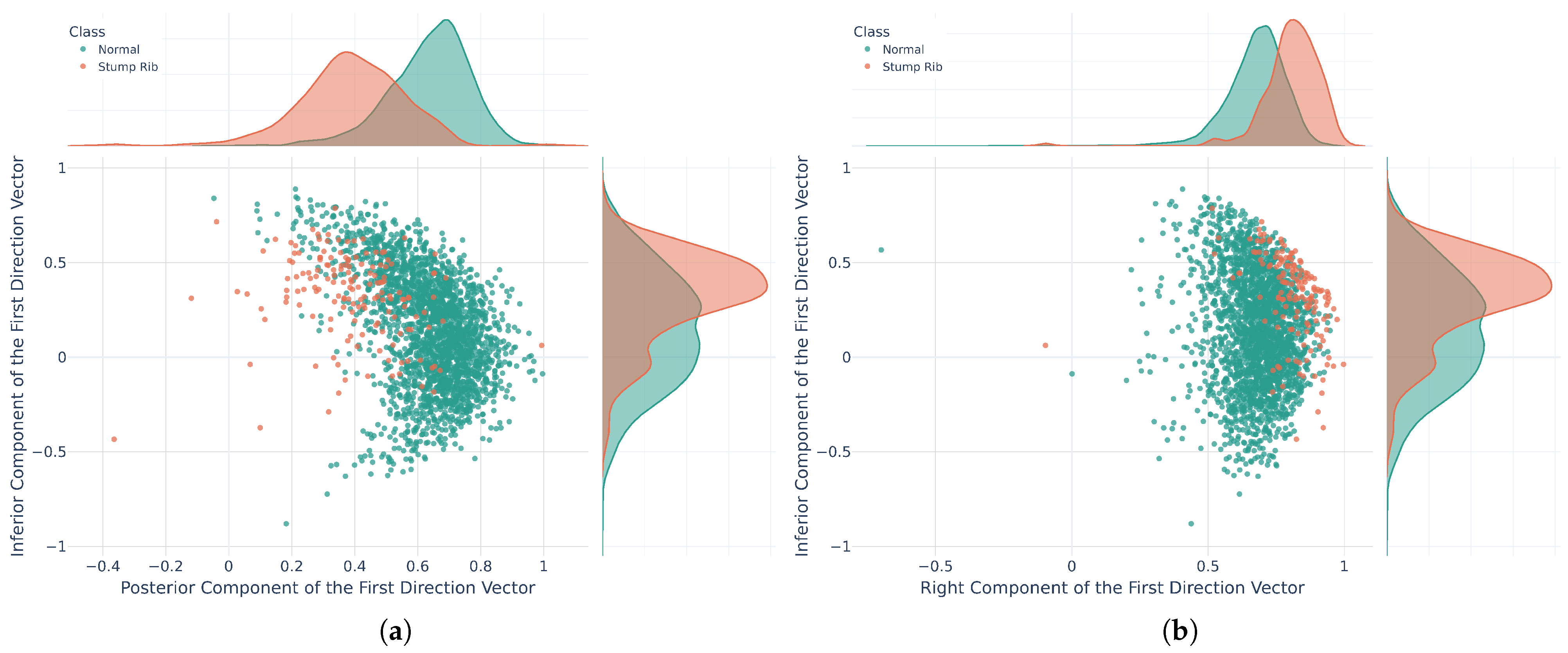
When observing the initial orientation of a rib by using the unit vector from the start point to the second path point (equivalent to 2-PPR, which is roughly the beginning 7 mm of a rib), we see significant differences. The posterior component of stump ribs is smaller ( 0.39 ± 0.17 vs. 0.64 ± 0.13 , p-value < 0.01), while the inferior component is higher ( 0.32 ± 0.23 vs. 0.15 ± 0.30 , p-value < 0.01). Additionally, stump ribs are more laterally angled (right component of 2-PPR 0.81 ± 0.11 vs. 0.68 ± 0.11 , p-value < 0.01). In summary, even in the first 7 mm of a rib, full-length ribs have a more prominent posterior component, meaning the ribs are angled more towards the back of the vertebra at the beginning. In contrast, stump ribs are more outwards and downwards oriented (see Figure 7).
Using the 4-PPR on each rib, a Support Vector Machine (SVM), trained with a polynomial kernel and random 70/30 splits, reaches an average F1-score of 0.77 ± 0.04 across 10 runs in distinguishing SR from non-SR (see Table 5). A multilayer perceptron (MLP) with the same setup achieves an F1-score of 0.84 ± 0.02 . Taking only the first three points (3-PPR) reduces the F1-score to 0.67 ± 0.05 for the polynomial SVM and to 0.71 ± 0.03 for the MLP. Using the relation between the rib start and the vertebra corpus surface and center (DRC) results in an F1-score of 0.59 ± 0.05 and 0.62 ± 0.06 with the same SVM and MLP setup, respectively. Although DRC alone as input does not perform as well, combining it with n-PPR mainly boosts the performance (see Table 5). Overall, the multilayer perceptron (MLP) and linear SVM achieve the best F1-scores, while logistic regression (LoRe) and a polynomial SVM often lag behind.
We achieved the best F1 performance of 0.84 by using both 4-PPR and DRC as inputs to an MLP or linear SVM.
For a study that analyzes the relation of the stump rib length threshold to the SVM performance, see Appendix D. For further experiments, including regressing the total rib length, precision and recall values, and stump rib classification based on the grayscale image, see Appendix E, Appendix F and Appendix G.

4. Discussion

Overall, our proposed method can robustly detect, localize, segment, and measure ribs in CT scans. This allows an automatic classification of stump ribs. Additionally, we propose simple morphological features beyond the length to correctly classify thoracolumbar stump ribs. These enable the detection of stump ribs in limited, arbitrary-field-of-view CT images and may help correctly label vertebrae and improve surgical planning.
Best stump-rib classification performance was achieved with both 4-PPR and DRC as feature inputs. Notably, to achieve this, we only require the beginning segment of the rib and the corresponding vertebra segmentation. This is fascinating, as the first four path points have an average total length of around 22 mm. By looking at the initial 22 mm of a rib’s direction and orientation, we can deduce whether the rib is a stump rib or not. If only the initial 15 mm (required for 3-PPR) of a rib is visible in the scan, we lose some performance but still get decent results. This is especially interesting in cases where the scan is not very wide, and thus, the ribs are not fully visible. Thus, our experiments imply that ribs can be categorized by morphological features, adding depth to the classification beyond a simple cutoff based on rib length.
However, limitations must be acknowledged. As there is no gold standard for manually measuring rib length, we cannot perform a quantitative comparative analysis of the exact measurements. Furthermore, the two public datasets VerSe and RibFrac used in this study have backgrounds in spinal anomalies such as fractures and rib cage fractures, respectively. Thus, they do not represent the general population, and we forfeit meaningful normative values or more generalized findings and relationships about ribs. Furthermore, our segmentation evaluation is restricted to only those datasets and does not contain an external test set. Correcting the predictions from the initial segmentation model might introduce a slight bias, which we do acknowledge. Compared to the literature, we observe more stump ribs in our data. We leave the correlation between rib lengths and the prevalence of stump ribs, along with other factors such as sex, height, and weight, for future work in a more representative cohort. Additionally, we did not compare nnUNet against other methods. Since we achieved excellent segmentation results, a comparison seemed unnecessary, and we provided the community with a simple, easy-to-use nnUNet.
Although this did not occur for the lowest two ribs in our analysis data, we acknowledge that the instance assignment algorithm will fail if ribs from adjacent vertebral levels are fused or connected in the segmentation.
The accuracy of the measured rib length depends on the quality of the segmentation masks produced. If the segmentation is erroneous, so is the measured rib length. However, in our experiments, we did not observe significant rib-length errors due to typical automatic segmentation inaccuracies. Only severe errors, such as merged ribs, large missing segments, split ribs, or structural anomalies (e.g., bone tumors or partially resected ribs), will result in measurable deviations due to algorithm design. Minor errors, i.e., those with a similar surface delineation, mostly result in length errors of less than 1 mm.
Finally, although we manually corrected all ribs and evaluated segmentation performance across all ribs in a scan, our downstream experiments focused on the lowest two ribs. Thus, we did not manually review measurements of the upper thoracic ribs and cannot guarantee the same level of measurement consistency there. However, as only the lowest ribs in a subject can be stump ribs, the measurement of the length is more important there.
We leave it to future research to include the morphology of the vertebra in a rib-focused analysis, accounting for abnormalities such as enlarged foveae. Additionally, a larger population study using our segmentation and rib-length measurement tools could further improve our understanding of stump ribs. Moreover, the occurrence of our stump rib features and their prevalence in relation to other aberrations, such as lumbosacral anomalies, should be investigated. Lastly, we leave open the question of whether the rib length measurement algorithm and morphological features can be used in an inverse manner to detect rib segmentation errors.

Finally, we make the code and model weights publicly available (https://github.com/Hendrik-code/rib-segmentation, accessed on 2 March 2026), thus making it easy for fellow researchers to create rib segmentation masks for their own data. Further, we release the manually corrected and predicted rib masks for the two public datasets, VerSe and RibFrac (https://doi.org/10.5281/zenodo.14850928).

Author Contributions

Conceptualization, H.M. and J.S.K.; methodology, H.M., A.D. and R.G.; software, H.M., R.G., M.A. and F.K.; validation, H.M., J.S.K., D.R., H.S. and R.G.; formal analysis, H.M., A.D., B.K.-W., J.P., F.J., R.B. and B.M.; investigation, H.M., A.D., B.K.-W., H.S. and J.S.K.; resources, A.D., B.K.-W., J.P., F.J., R.B., B.M., D.R. and J.S.K.; data curation, H.S., A.D., B.K.-W., J.P., F.J. and R.B.; writing—original draft preparation, H.M., A.D., H.S., M.A. and R.G.; writing—review and editing, all co-authors.; visualization, H.M., H.S., R.G., M.A. and F.K.; supervision, H.S., J.S.K., B.M., R.B. and D.R.; project administration, D.R. and J.S.K.; funding acquisition, D.R. and J.S.K. All authors have read and agreed to the published version of the manuscript.

Funding

This study has received funding from the European Research Council (ERC) under the European Union’s Horizon 2020 research and innovation program (101045128—iBack-epic—ERC2021-COG).

Institutional Review Board Statement

The study was approved by the Ethics Committee of Technical University of Munich (27/19 S-SR dated 22 April 2020 ).

Informed Consent Statement

The local ethics committee waived informed consent, 27/19 S-SR dated 22 April 2020.

Data Availability Statement

The created manual and predicted segmentation masks from this study are published under https://doi.org/10.5281/zenodo.14850928. The corresponding CT images are from public datasets, accessible at https://github.com/anjany/verse and https://zenodo.org/records/3893508, both accessed on 2 March 2026.

Acknowledgments

During the preparation of this manuscript/study, the author(s) used Grammarly for the purposes of refining the language of the written text. The authors have reviewed and edited the output and take full responsibility for the content of this publication.

Conflicts of Interest

Jan Kirschke reports a non-financial relation. He is a co-founder and shareholder of Bonescreen GmbH (see https://bonescreen.de/ accessed on 2 March 2026). During this study, the authors who analyzed and controlled the data were not employees, co-founders, or shareholders of Bonescreen GmbH. The remaining authors declare that the research was conducted in the absence of any commercial or financial relationships that could be construed as a potential conflict of interest.

Abbreviations

The following abbreviations are used in this manuscript:
CTComputed Tomography
SRStump rib
TLTVThoracolumbar Transitional Vertebra
RLMARib Length Measurement Algorithm
DRCDirection Rib Corpus
PDRCPosterior Component of the DRC vector
n-PPRThe 3D spatial relation vectors of the first n path points
TSTotalSegmentator
DSCDice similarity coefficient
ASSDAverage symmetric surface distance
RQRecognition Quality
SQSegmentation Quality
PQPanoptic Quality
IoUIntersection over Union
SVMSupport Vector Machine
MLPMultilayer Perceptron
LoReLogistic Regression

Appendix A. Evaluation Metrics

We evaluated the rib segmentations produced by our model using multiple metrics.
Dice similarity coefficient (DSC): It is a crucial overlap score that measures how many voxels between the prediction and the reference annotation match. Given X and Y as the predicted and reference annotations, respectively, we can calculate the DSC using Equation (A1).
DSC ( X , Y ) = 2 | X Y | | X | + | Y | [ 0 , 1 ]
Average symmetric surface distance (ASSD): This metric reports the average of all the distances from points on the boundary of the predicted annotation to the boundary of the reference annotation, and vice versa. With d ( a , b ) being the distance between two points a and b, and A, B being the boundaries of X and Y, respectively, we can calculate the ASSD via Equation (A2). ASSD is important for showing how far erroneous or missing voxels are from the reference annotation, i.e., whether errors are local.
ASSD ( X , Y ) = asd ( A , B ) + asd ( B , A ) | X | + | Y | [ 0 , ]
asd ( A , B ) = a A min b B d ( a , b ) [ 0 , ]
Utilizing panoptica [27], we match instances with a DSC greater than or equal to 0.5 as true positives. With that in mind, we calculate the following instance-wise metrics:
Recognition Quality (RQ): The F1-score of instance detection based on the above definition of true positives. With tp, fp, and fn being true positives, false positives, and false negatives, respectively, we calculate the RQ via Equation (A4). This score indicates the quality of rib detection.
RQ ( tp , fp , fn ) = tp tp + 1 2 · ( fp + fn ) [ 0 , 1 ]
With a metric M, we define the segmentation quality ( SQ M ) as the average of the metric M across all true positives, defined by Equation (A5). This yields how well the detected instances have been segmented.
SQ M ( tp ) = ( i ref , i pred ) tp M ( i ref , i pred ) | tp |
Finally, the panoptic quality (PQ) combines the RQ and SQ. Again using a metric M, we define the PQ with Equation (A6).
PQ M ( X , Y ) = SQ M · RQ
We evaluate the rib segmentation model using the DSC on the whole masks, i.e., calculating a binary overlap score (binary DSC), as well as the instance-wise metrics RQ, SQ DSC , PQ DSC , and SQ ASSD for a detailed comparison.

Appendix B. Qualitative Failure Analysis

Based on our analysis set of 2464 individual ribs across 648 subjects, we had noticeable segmentation errors in 1.8% of them.
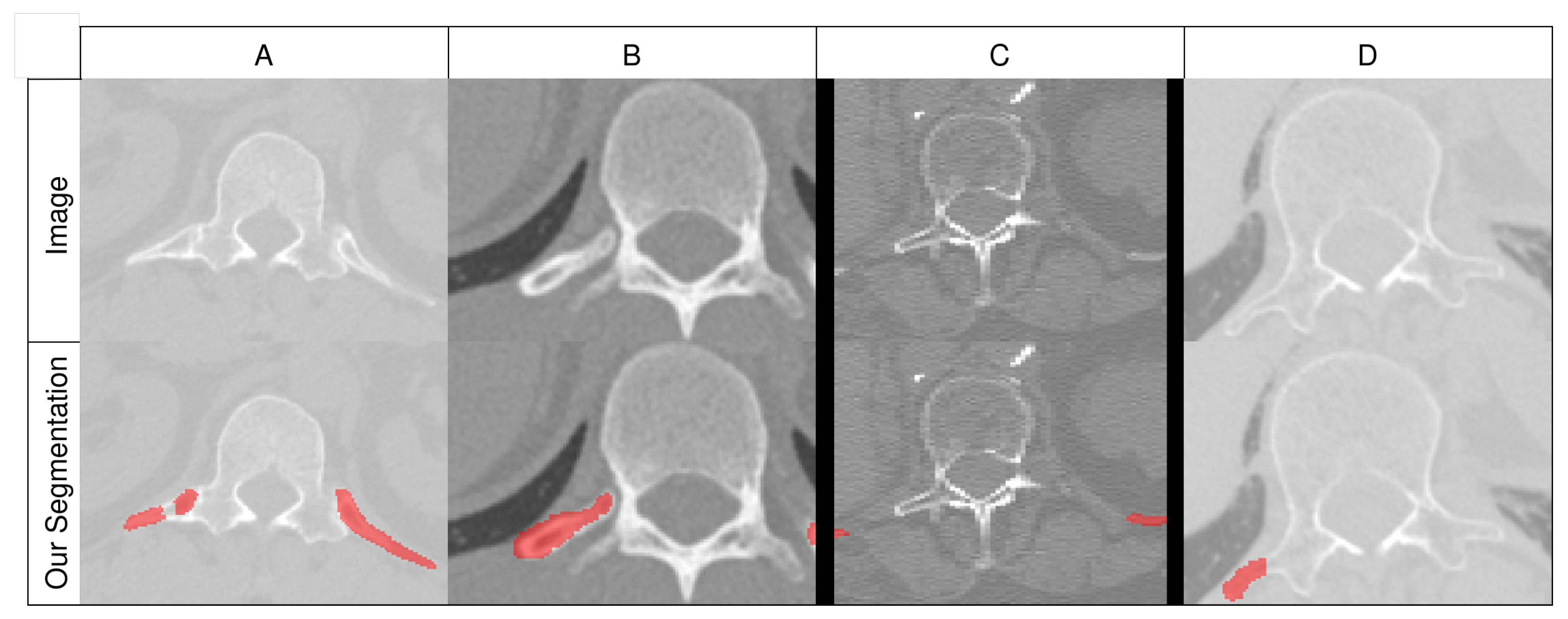
Figure A1. Examples of challenging and failure cases. The top row portrays the image, and the bottom overlays our predicted segmentation. (A) A challenging case where the distinction between costal process and rib is unclear due to fusion. The two components are joined in other slices, and the measured rib length would not have influenced the SR label. (B) Imperfect segmentation quality that did not affect the measured rib length. (C) A scan that is not wide enough to fully capture the ribs (the left and right black areas are the image’s ends). The measured rib length of the visible parts is correct; thus, we know if it is not an SR if that length already exceeds the threshold. (D) An error where the segmentation model confused the costal process with a rib and segmented it, detecting a rib where there isn’t.
Ai 07 00224 g0a1
Figure A1 demonstrates the typical cases we observed. Most segmentation errors are small and local and do not noticeably influence the measured rib length. The failure cases consist primarily of samples with fusion; thus, distinguishing the costal process from the rib is rather challenging. For one case, the model segmented the costal process of a lumbar vertebra. We can only hypothesize that this is an edge case where the costal process and surrounding image structures resemble a rib.
In the future, extracting precise vertebra labels from vertebra labeling approaches and using them to eliminate these rarely segmented costal processes could be an automated way to detect these errors. Another approach could be to calculate normative values from large amounts of manually checked data, then detect outliers by comparing the features against the normative distribution.

Appendix C. Effect of Segmentation Quality on the Rib Length

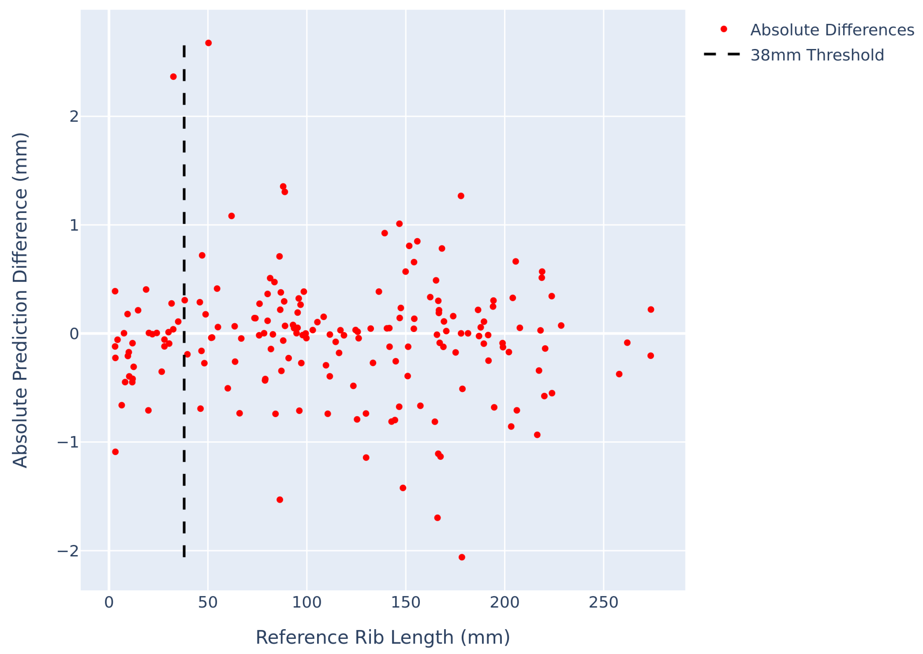
Figure A2 compares the rib length derived from the predicted segmentation annotations to those from the reference annotations for the test set of 45 subjects. This analysis was again performed only on the lowest two ribs. Most differences are below 1 mm. There is only one sample where the difference would change the stump rib label.
Figure A2. The absolute difference in measured rib length between the predicted and reference segmentation annotations on the test set. The dotted black line marks the common stump rib threshold.
Ai 07 00224 g0a2

Appendix D. Moving Stump Rib Threshold

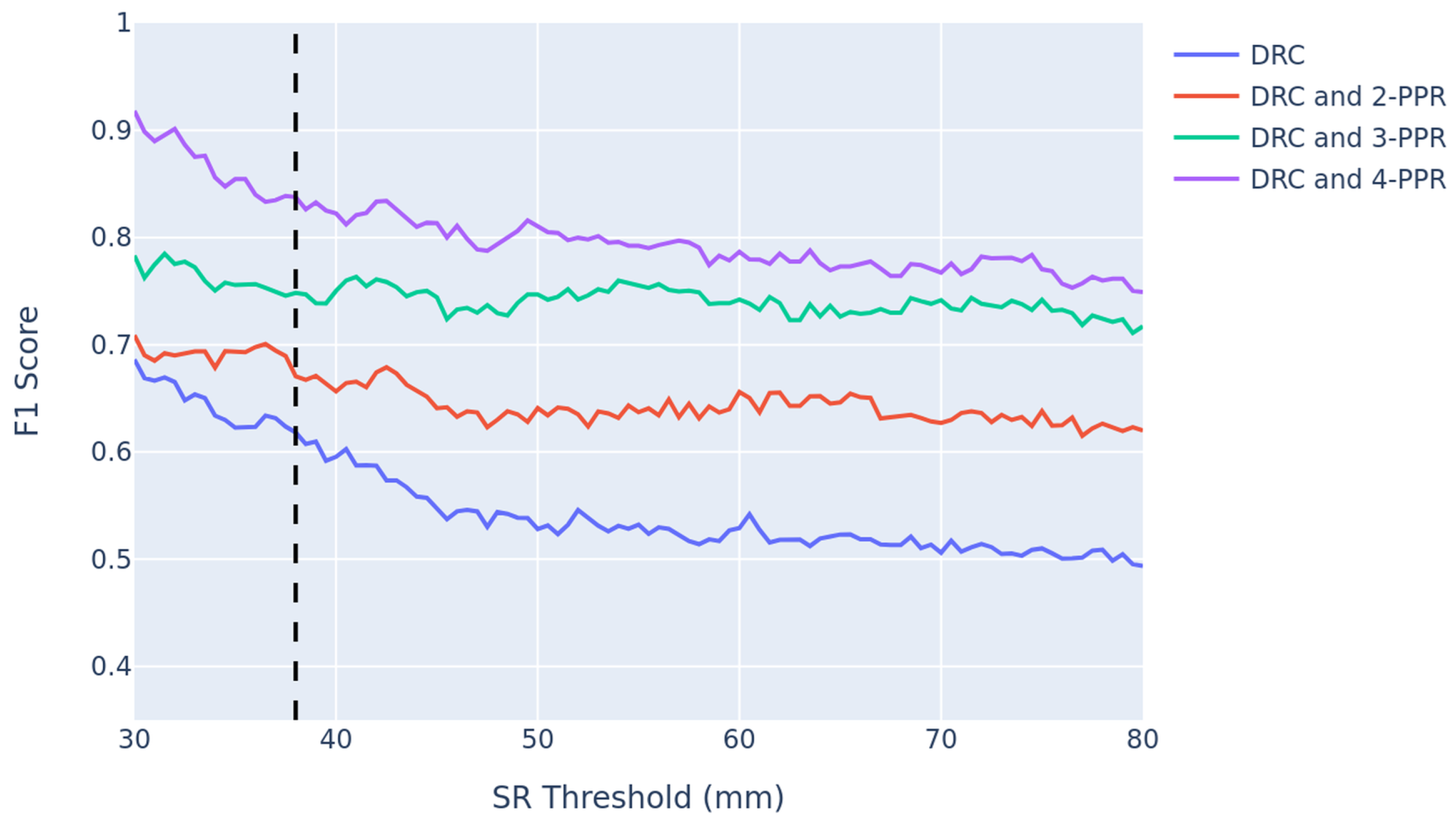
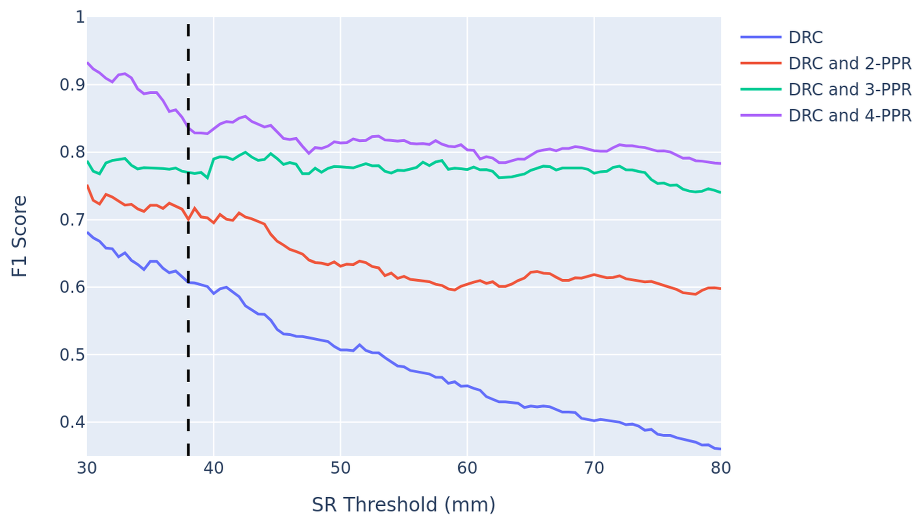
The length threshold defined for stump ribs is 38 mm. When experimenting with different shifts to this threshold to generate the binary labels, the F1-score using 4-PPR and DRC is consistently above all other sets of inputs (see Figure A3 and Figure A4). Using three points is still consistently better than using only the first two path points. As the threshold increases, performance mostly decreases. Please note that an F1-score of 0.5 means that the two classes (SR and non-SR) are not distinguishable by the features.
Although the 38 mm stump rib threshold has been adopted from prior literature as a clinically relevant cutoff, we cannot demonstrate a distinct peak or transition at this value. This suggests that the relationship may be more continuous rather than reflecting a strict biological threshold. Nevertheless, we retained the 38 mm cutoff to ensure comparability with previous studies and because it remains the most commonly reported reference value in the field. These findings should therefore be interpreted with caution, and alternative thresholds or continuous modeling approaches need to be discussed in further studies.
Figure A3. The relation of the classification performance of a linear SVM and the stump rib threshold used to create the reference SR labels. The x-axis shows the SR threshold in mm, while the y-axis is the average F1 score over 10 runs. The dashed black line highlights the generally defined length threshold of 38 mm.
Ai 07 00224 g0a3
Figure A4. The relation of the classification performance of an MLP and the stump rib threshold used to create the reference SR labels. The x-axis shows the SR threshold in mm, while the y-axis is the average F1 score over 10 runs. The dashed black line highlights the generally defined length threshold of 38 mm.
Ai 07 00224 g0a4

Appendix E. Rib Length Regression

We were interested in whether we could extend the classification by regressing the length of the entire rib. For this, as with SVMs for classification, we use linear regression, linear SVM, polynomial SVM, and an MLP to evaluate regression performance using our proposed features (see Table A1). For better stability, we divided the length by ten to yield centimeters instead of millimeters.
The MLP outperforms every other architecture on every metric and feature set. Although one could argue that the best MAE of 2.33 ± 0.07 is good in the context of whole rib length estimation, it is poor in the context of stump rib detection. On average, we are more than half a stump rib’s length wrong for this regression. When interested in stump rib detection, we cannot recommend this approach. In the general context of measuring rib length, it is notable that, given our limited field-of-view feature values, an MLP regressor at least gets into the right order of magnitude.
Table A1. Evaluation of the models trained on morphological features to regress the rib length based on incomplete information. We report the mean (rooted) MSE, MAE, and R2, along with their standard deviations, across 10 runs with different seeds. The value in bold marks the best-performing combination for each feature and metric. The arrow after the metric indicates whether higher or lower values are better.
MetricLinear RegressionLinear SVMPolynomial SVMMLP
MSE ↓
DRC 4.36 ± 0.09 4.37 ± 0.06 15.54 ± 18.86 4 . 32 ± 0.14
2-PPR 4.06 ± 0.1 4.04 ± 0.09 5.14 ± 0.92 3 . 87 ± 0.08
3-PPR 3.78 ± 0.15 3.83 ± 0.17 6.74 ± 3.44 3 . 53 ± 0.11
4-PPR 3.58 ± 0.16 3.66 ± 0.22 5.82 ± 1.94 3 . 33 ± 0.1
DRC and 2-PPR 3.64 ± 0.17 3.62 ± 0.12 4.64 ± 0.61 3 . 44 ± 0.11
DRC and 3-PPR 3.45 ± 0.2 3.43 ± 0.17 5.71 ± 2.55 3 . 15 ± 0.11
DRC and 4-PPR 3.36 ± 0.24 3.35 ± 0.2 5.96 ± 3.28 3 . 12 ± 0.19
MAE ↓
DRC 3.45 ± 0.06 3.48 ± 0.05 4.3 ± 0.8 3 . 35 ± 0.05
2-PPR 3.14 ± 0.07 3.13 ± 0.07 3.56 ± 0.15 2 . 99 ± 0.06
3-PPR 2.91 ± 0.06 2.92 ± 0.07 3.54 ± 0.22 2 . 7 ± 0.07
4-PPR 2.77 ± 0.07 2.79 ± 0.08 3.42 ± 0.17 2 . 55 ± 0.06
DRC and 2-PPR 2.79 ± 0.07 2.8 ± 0.07 3.28 ± 0.11 2 . 67 ± 0.06
DRC and 3-PPR 2.62 ± 0.06 2.62 ± 0.06 3.28 ± 0.18 2 . 41 ± 0.06
DRC and 4-PPR 2.54 ± 0.07 2.54 ± 0.07 3.27 ± 0.22 2 . 33 ± 0.07
R2 ↑
DRC 0.41 ± 0.03 0.41 ± 0.03 17.07 ± 36.0 0 . 42 ± 0.05
2-PPR 0.49 ± 0.03 0.49 ± 0.02 0.15 ± 0.34 0 . 54 ± 0.02
3-PPR 0.56 ± 0.04 0.55 ± 0.04 0.75 ± 1.85 0 . 62 ± 0.02
4-PPR 0.6 ± 0.04 0.58 ± 0.05 0.16 ± 0.79 0 . 66 ± 0.02
DRC and 2-PPR 0.59 ± 0.04 0.59 ± 0.03 0.33 ± 0.17 0 . 63 ± 0.03
DRC and 3-PPR 0.63 ± 0.05 0.63 ± 0.04 0.21 ± 1.28 0 . 69 ± 0.02
DRC and 4-PPR 0.65 ± 0.05 0.65 ± 0.05 0.41 ± 1.65 0 . 7 ± 0.04

Appendix F. Image-Based Stump-Rib Classification

As an additional ablation, we trained a standard Convolutional Neural Network (CNN) and a Vision Transformer (ViT) for stump rib classification. To this end, we trained on CT grayscale images rather than morphological features. Using the same train/test splits repeated over 10 random seeds, we report the mean and standard deviation across folds.
Since we cannot perfectly cut the field of view to achieve scientific comparability with classifiers based on morphological features, we decided to run two experiments: Once cropping the ribs to simulate the length of the rib required for 4-PPR, and once on the whole rib as an upper-bounds estimation. We pad accordingly to ensure a consistent cutout size across all samples.
In detail, we used a compact four-stage 3D CNN with dropout of 0.3, the 3D Vision Transformer from MONAI with 6 layers and dropout of 0.1. We trained with AdamW, a learning rate of 1 × 10 4 , weight decay of 1 × 10 4 , class-weighted cross-entropy, and a batch size of 8.
The results (see Table A2) show that while a Vision Transformer lags behind, a 3D CNN trained on the grayscale images cut to individual ribs based on a given segmentation has comparable performance in classifying stump ribs. Models trained on the whole rib yield outstanding performance, providing a strong upper bound in scenarios where the field of view covers the whole rib.
Table A2. Evaluation of the imaging-based models for classifying stump ribs against regular ribs. We report mean balanced accuracy, AUC, F1-score, precision and recall with standard deviations across 10 seeds. Arrows indicate whether higher or lower is better.
Model3D CNNViT3D CNNViT
Config Cut Rib Cut Rib Whole Rib Whole Rib
Balanced Accuracy ↑ 0.92 ± 0.03 0.80 ± 0.04 0.96 ± 0.01 0.95 ± 0.02
AUC ↑ 0.99 ± 0.00 0.95 ± 0.02 1.00 ± 0.00 1.00 ± 0.00
F1 ↑ 0.84 ± 0.03 0.68 ± 0.06 0.90 ± 0.02 0.86 ± 0.05
Precision ↑ 0.82 ± 0.03 0.77 ± 0.06 0.86 ± 0.04 0.81 ± 0.06
Recall ↑ 0.85 ± 0.06 0.62 ± 0.08 0.96 ± 0.03 0.92 ± 0.04

Appendix G. Precision and Recall

Since the result section only provides F1-score, here are the detailed precision and recall values for the same experiments.
Table A3. Evaluation of the classifiers trained on morphological features to classify stump ribs against regular ribs. We report the mean precision and recall, along with their standard deviations, across 10 runs with different seeds. The arrows after the metric name indicate whether higher or lower values are better. The value in bold marks the best-performing architecture for each feature and metric.
FeaturesLinear SVMPolynomial SVMLoReMLP
Precision ↑
DRC 0.89 ± 0.09 0 . 9 ± 0.05 0.8 ± 0.1 0.74 ± 0.11
2-PPR 0 . 98 ± 0.03 0.84 ± 0.09 0.8 ± 0.06 0.79 ± 0.08
3-PPR 0.8 ± 0.08 0.8 ± 0.06 0 . 81 ± 0.06 0.76 ± 0.07
4-PPR 0 . 95 ± 0.04 0.93 ± 0.04 0.87 ± 0.07 0.87 ± 0.05
DRC and 2-PPR 0 . 86 ± 0.07 0.75 ± 0.06 0.82 ± 0.06 0.7 ± 0.08
DRC and 3-PPR 0.82 ± 0.08 0.79 ± 0.08 0 . 83 ± 0.08 0.76 ± 0.06
DRC and 4-PPR 0 . 91 ± 0.06 0.87 ± 0.06 0.88 ± 0.06 0.86 ± 0.06
Recall ↑
DRC 0.47 ± 0.07 0.44 ± 0.06 0.52 ± 0.08 0 . 54 ± 0.07
2-PPR 0.23 ± 0.05 0.37 ± 0.05 0.43 ± 0.05 0 . 45 ± 0.06
3-PPR 0.62 ± 0.06 0.58 ± 0.08 0.66 ± 0.05 0 . 67 ± 0.06
4-PPR 0.76 ± 0.02 0.66 ± 0.04 0.79 ± 0.04 0 . 81 ± 0.03
DRC and 2-PPR 0.59 ± 0.06 0.54 ± 0.06 0.62 ± 0.06 0 . 65 ± 0.06
DRC and 3-PPR 0 . 74 ± 0.08 0.62 ± 0.07 0.73 ± 0.07 0 . 74 ± 0.05
DRC and 4-PPR 0.78 ± 0.03 0.68 ± 0.05 0.79 ± 0.04 0 . 82 ± 0.06

References

  1. Thawait, G.K.; Chhabra, A.; Carrino, J.A. Spine segmentation and enumeration and normal variants. Radiol. Clin. N. Am. 2012, 50, 587–598. [Google Scholar] [CrossRef] [PubMed]
  2. Tatara, Y.; Niimura, T.; Sekiya, T.; Mihara, H. Changes in lumbosacral anatomy and vertebral numbering in patients with thoracolumbar and/or lumbosacral transitional vertebrae. JBJS Open Access 2021, 6, e20. [Google Scholar] [CrossRef] [PubMed]
  3. Wigh, R.E. The thoracolumbar and lumbosacral transitional junctions. Spine 1980, 5, 215–222. [Google Scholar] [CrossRef] [PubMed]
  4. Kim, B.G.; Dan, J.M.; Shin, D.E. Treatment of thoracolumbar fracture. Asian Spine J. 2015, 9, 133. [Google Scholar] [CrossRef] [PubMed]
  5. Du Plessis, A.M.; Greyling, L.M.; Page, B.J. Differentiation and classification of thoracolumbar transitional vertebrae. J. Anat. 2018, 232, 850–856. [Google Scholar] [CrossRef] [PubMed]
  6. Poolman, A.M.; Wessels, Q.; Schoor, A.V.; Keough, N. Thoracolumbar transitional vertebrae: Quantitative differentiation and associated numeric variation in the vertebral column using skeletal remains. J. Anat. 2023, 243, 311–318. [Google Scholar] [CrossRef] [PubMed]
  7. Mahato, N.K. Thoracolumbar transitional vertebrae: Stages of osteological transition, mechanism of changes in zygapophyseal loading and orientation, and assimilation of mammillary processes. J. Anat. 2018, 233, 394. [Google Scholar] [CrossRef] [PubMed]
  8. Csurka, G.; Volpi, R.; Chidlovskii, B. Semantic image segmentation: Two decades of research. Found. Trends Comput. Graph. Vis. 2022, 14, 1–162. [Google Scholar] [CrossRef]
  9. Isensee, F.; Jaeger, P.F.; Kohl, S.A.; Petersen, J.; Maier-Hein, K.H. nnU-Net: A self-configuring method for deep learning-based biomedical image segmentation. Nat. Methods 2021, 18, 203–211. [Google Scholar] [PubMed]
  10. Shen, H.; Liang, L.; Shao, M.; Qing, S. Tracing based segmentation for the labeling of individual rib structures in chest CT volume data. In Proceedings of the Medical Image Computing and Computer-Assisted Intervention–MICCAI 2004: 7th International Conference, Saint-Malo, France, 26–29 September 2004; Springer: Berlin/Heidelberg, Germany, 2004; pp. 967–974. [Google Scholar]
  11. Klinder, T.; Lorenz, C.; Von Berg, J.; Dries, S.P.; Bülow, T.; Ostermann, J. Automated model-based rib cage segmentation and labeling in CT images. In Proceedings of the International Conference on Medical Image Computing and Computer-Assisted Intervention; Springer: Berlin/Heidelberg, Germany, 2007; pp. 195–202. [Google Scholar]
  12. Wu, M.; Chai, Z.; Qian, G.; Lin, H.; Wang, Q.; Wang, L.; Chen, H. Development and evaluation of a deep learning algorithm for rib segmentation and fracture detection from multicenter chest CT images. Radiol. Artif. Intell. 2021, 3, e200248. [Google Scholar] [CrossRef] [PubMed]
  13. Staal, J.; van Ginneken, B.; Viergever, M.A. Automatic rib segmentation and labeling in computed tomography scans using a general framework for detection, recognition and segmentation of objects in volumetric data. Med. Image Anal. 2007, 11, 35–46. [Google Scholar] [CrossRef] [PubMed]
  14. Lenga, M.; Klinder, T.; Bürger, C.; von Berg, J.; Franz, A.; Lorenz, C. Deep learning based rib centerline extraction and labeling. In Proceedings of the Computational Methods and Clinical Applications in Musculoskeletal Imaging: 6th International Workshop, MSKI 2018, Held in Conjunction with MICCAI 2018, Granada, Spain, 16 September 2018; Springer: Berlin/Heidelberg, Germany, 2019; pp. 99–113. [Google Scholar]
  15. Wu, D.; Liu, D.; Puskas, Z.; Lu, C.; Wimmer, A.; Tietjen, C.; Soza, G.; Zhou, S.K. A learning based deformable template matching method for automatic rib centerline extraction and labeling in CT images. In Proceedings of the 2012 IEEE Conference on Computer Vision and Pattern Recognition, Providence, RI, USA, 16–21 June 2012; IEEE: Piscataway, NJ, USA, 2012; pp. 980–987. [Google Scholar]
  16. Wang, W.; Feng, H.; Bu, Q.; Cui, L.; Xie, Y.; Zhang, A.; Feng, J.; Zhu, Z.; Chen, Z. MDU-Net: A Convolutional Network for Clavicle and Rib Segmentation from a Chest Radiograph. J. Healthc. Eng. 2020, 2020, 2785464. [Google Scholar] [CrossRef] [PubMed]
  17. Ramakrishnan, S.; Alvino, C.; Grady, L.; Kiraly, A. Automatic three-dimensional rib centerline extraction from CT scans for enhanced visualization and anatomical context. In Proceedings of the Medical Imaging 2011: Image Processing; SPIE: Bellingham, WA, USA, 2011; Volume 7962, pp. 922–933. [Google Scholar]
  18. Wasserthal, J.; Breit, H.C.; Meyer, M.T.; Pradella, M.; Hinck, D.; Sauter, A.W.; Heye, T.; Boll, D.T.; Cyriac, J.; Yang, S.; et al. TotalSegmentator: Robust segmentation of 104 anatomic structures in CT images. Radiol. Artif. Intell. 2023, 5, e230024. [Google Scholar] [CrossRef] [PubMed]
  19. Sekuboyina, A.; Husseini, M.E.; Bayat, A.; Löffler, M.; Liebl, H.; Li, H.; Tetteh, G.; Kukačka, J.; Payer, C.; Štern, D.; et al. VerSe: A vertebrae labelling and segmentation benchmark for multi-detector CT images. Med. Image Anal. 2021, 73, 102166. [Google Scholar] [PubMed]
  20. Jin, L.; Yang, J.; Kuang, K.; Ni, B.; Gao, Y.; Sun, Y.; Gao, P.; Ma, W.; Tan, M.; Kang, H.; et al. Deep-Learning-Assisted Detection and Segmentation of Rib Fractures from CT Scans: Development and Validation of FracNet. EBioMedicine 2020, 62, 103106. [Google Scholar] [PubMed]
  21. Yang, J.; Shi, R.; Jin, L.; Huang, X.; Kuang, K.; Wei, D.; Gu, S.; Liu, J.; Liu, P.; Chai, Z.; et al. Deep Rib Fracture Instance Segmentation and Classification from CT on the RibFrac Challenge. arXiv 2024, arXiv:2402.09372. [Google Scholar]
  22. Jin, L.; Gu, S.; Wei, D.; Adhinarta, J.K.; Kuang, K.; Zhang, Y.J.; Pfister, H.; Ni, B.; Yang, J.; Li, M. Ribseg v2: A large-scale benchmark for rib labeling and anatomical centerline extraction. IEEE Trans. Med. Imaging 2023, 43, 570–581. [Google Scholar]
  23. Yushkevich, P.A.; Piven, J.; Hazlett, H.C.; Smith, R.G.; Ho, S.; Gee, J.C.; Gerig, G. User-guided 3D active contour segmentation of anatomical structures: Significantly improved efficiency and reliability. Neuroimage 2006, 31, 1116–1128. [Google Scholar] [CrossRef] [PubMed]
  24. Sekuboyina, A.; Rempfler, M.; Kukačka, J.; Tetteh, G.; Valentinitsch, A.; Kirschke, J.S.; Menze, B.H. Btrfly net: Vertebrae labelling with energy-based adversarial learning of local spine prior. In Proceedings of the Medical Image Computing and Computer Assisted Intervention–MICCAI 2018: 21st International Conference, Granada, Spain, 16–20 September 2018; Proceedings, Part IV 11; Springer: Berlin/Heidelberg, Germany, 2018; pp. 649–657. [Google Scholar]
  25. Cortes, C.; Vapnik, V. Support-vector networks. Mach. Learn. 1995, 20, 273–297. [Google Scholar] [CrossRef]
  26. Rey, D.; Neuhäuser, M. Wilcoxon-Signed-Rank Test. In International Encyclopedia of Statistical Science; Springer: Berlin/Heidelberg, Germany, 2011; pp. 1658–1659. [Google Scholar] [CrossRef]
  27. Kofler, F.; Möller, H.; Buchner, J.A.; de la Rosa, E.; Ezhov, I.; Rosier, M.; Mekki, I.; Shit, S.; Negwer, M.; Al-Maskari, R.; et al. Panoptica–instance-wise evaluation of 3D semantic and instance segmentation maps. arXiv 2023, arXiv:2312.02608. [Google Scholar]
Figure 1. The flow of our three utilized datasets. We used the private in-house dataset solely for training rib segmentation and performed all downstream experiments on public data. n always yields the number of samples. In the case of multiple values, they indicate the number of samples from different datasets.
Ai 07 00224 g001
Figure 2. Two example subjects (A+B) of the RibFrac dataset. We compare the original RibSeg annotation with the TotalSegmentator prediction and our rib segmentation model. Both the RibSeg annotation and the one from TotalSegmentator fail to annotate the rib part close to the vertebra. Furthermore, the RibSeg annotation is not dense, containing only the outline, whereas the one from TotalSegmentator lacks detail because it segments at an isotropic resolution of 1.5 mm. Our model is trained for 0.8 mm isotropic space; thus, it produces smooth and high-resolution annotations. This behavior is true for all samples in our datasets.
Ai 07 00224 g002
Figure 3. An example showing our transition from semantic rib segmentation to instance rib segmentation by using the vertebra instance segmentation provided by SpineR. From left to right: Binary rib segmentation; vertebra instance segmentation; resulting combined instance annotation. The colors represent distinct instances.
Ai 07 00224 g003
Figure 4. 2D Schematic illustration of our 3D rib length measurement algorithm (RLMA). The blue contour represents the rib, while the corresponding vertebra is orange (the vertebral corpus is darker). The first row shows the initialization of the starting point. First, we find the closest point of the rib surface to the center of the corresponding vertebra corpus (a); second, we use the surrounding points to find an average starting position (b), and third, we finalize the starting point by projecting back to the rib surface (c). The second row shows an iteration: finding candidate points within a fixed circular distance (d), taking the average of those candidate points, and then finding the next point on the path using the direction vector of the previous point and the average of the candidate points (e). The last panel (f) shows the example after the RLMA has calculated all path points. The figure demonstrates the algorithm in two dimensions for clarity, while the RLMA operates on three-dimensional data.
Ai 07 00224 g004
Figure 5. Example 2D image to showcase some of our calculated 3D features. Blue is the rib, and orange is its corresponding vertebra. The spatial relation between the rib start point (green point) and the center of the vertebral corpus region (blue point on dark orange) is denoted Direction Rib Corpus (DRC). PDRC is the posterior component of the DRC vector. The spatial relation for the first two path points is denoted 2-PPR (Path Point Relation, i.e., the direction vector between the start point and the next path point).
Ai 07 00224 g005
Figure 6. Analyzed ribs classes are colored as follows: SR (orange) and regular rib (blue). The x-axis shows the volume of a rib divided by its length, and the y-axis shows the PDRC. Although not separated, we observe a clear trend: stump ribs have a lower volume-to-length ratio and a greater posterior distance between the corpus and the rib, i.e., the rib starts further back. Outside the plot are density distribution curves.
Ai 07 00224 g006
Figure 7. Our analyzed rib classes are colored as follows: SR (orange) and regular rib (blue). The two axes show the components of the vector from the rib’s starting point to its first path point, normalized to a unit vector. We contrast the inferior component with the posterior (a) and right components (b). Outside the plot are density distribution curves.
Ai 07 00224 g007
Table 1. The data demographics of this study. We used the public VerSe and RibFrac data and a private in-house dataset.
VerSe [19]RibFrac [20]In-House Data
Subjects323420413
Sex (% female)N/A3650
Age range (yrs)≥1821–94≥18
Mean age (yrs) ± SD 59 ± 17 55 ± 12 69 ± 9
Date range (yrs)2013–2020N/A2016–2020
Backgroundspinal anomaliesfractured ribspre-treatment CT
Table 2. Evaluation of 45 manually corrected test subjects from the RibFrac and VerSe dataset on the rib segmentation task. We evaluate the TotalSegmentator (TS) model against our rib segmentation model. We report the mean and standard deviation. The arrow after the metric indicates whether higher or lower values are better. The TotalSegmentator cannot segment the rib’s beginning, as reflected in these metrics.
TS [18]Ours
Binary DSC ↑ 0.751 ± 0.078 0.997 ± 0.006
RQ 0.948 ± 0.054 0.987 ± 0.053
SQ DSC 0.738 ± 0.076 0.984 ± 0.043
PQ DSC 0.700 ± 0.080 0.971 ± 0.050
SQ ASSD 1.896 ± 1.167 0.064 ± 0.126
Table 3. Evaluation of the 20 manually corrected test subjects from the RibFrac dataset on the rib segmentation task. We evaluate the TS model, the official RibSeg annotations, and our rib segmentation model, both with and without holes filled (HF). We report the mean and standard deviation. The arrow after the metric indicates whether higher or lower values are better.
RibSegRibSeg HFTS [18]Ours
Binary DSC ↑ 0.644 ± 0.059 0.754 ± 0.056 0.779 ± 0.017 0.999 ± 0.003
RQ 0.974 ± 0.031 0.974 ± 0.031 0.961 ± 0.044 0.976 ± 0.033
SQ DSC 0.647 ± 0.059 0.747 ± 0.057 0.761 ± 0.029 0.990 ± 0.020
PQ DSC 0.630 ± 0.059 0.728 ± 0.060 0.732 ± 0.054 0.967 ± 0.044
SQ ASSD 1.931 ± 0.485 1.840 ± 0.483 1.916 ± 0.478 0.071 ± 0.143
Table 4. Quantitative results of the manual review of the lowest ribs across RibFrac and VerSe data. The majority of segmentations were correct or showed only minor errors, which did not influence the length measurement algorithm. The percentages are all compared to the total number of ribs analyzed and reviewed. Each block separated by a horizontal line sums to 100%.
Percentage
Ribs rated (5)69.3
Ribs rated (4)16.7
Ribs rated (3)12.2
Ribs rated (2)1.2
Ribs rated (1)0.6
Ribs have correct measure98.2
Ribs incorrectly segmented1.8
Table 5. Evaluation of the classifiers trained on morphological features to classify stump ribs against regular ribs. We report the mean F1-score, balanced accuracy, and area under the curve (AUC), along with their standard deviations, across 10 runs with different seeds. The arrows after the metric name indicate whether higher or lower values are better. The value in bold marks the best-performing architecture for each feature and metric.
FeaturesLinear SVMPolynomial SVMLoReMLP
Balanced Accuracy ↑
DRC 0.73 ± 0.03 0.72 ± 0.03 0.75 ± 0.04 0 . 76 ± 0.04
2-PPR 0.61 ± 0.03 0.68 ± 0.02 0.71 ± 0.02 0 . 72 ± 0.03
3-PPR 0.81 ± 0.03 0.79 ± 0.04 0.82 ± 0.03 0 . 83 ± 0.03
4-PPR 0.88 ± 0.01 0.83 ± 0.02 0.89 ± 0.02 0 . 9 ± 0.01
DRC and 2-PPR 0.79 ± 0.03 0.76 ± 0.03 0 . 81 ± 0.03 0 . 81 ± 0.03
DRC and 3-PPR 0 . 86 ± 0.04 0.8 ± 0.03 0 . 86 ± 0.03 0 . 86 ± 0.02
DRC and 4-PPR 0.89 ± 0.02 0.84 ± 0.03 0.89 ± 0.02 0 . 91 ± 0.03
Area under Curve (AUC) ↑
DRC 0.94 ± 0.02 0.84 ± 0.03 0 . 95 ± 0.02 0.94 ± 0.02
2-PPR 0 . 92 ± 0.02 0.87 ± 0.03 0 . 92 ± 0.02 0 . 92 ± 0.02
3-PPR 0 . 97 ± 0.02 0.91 ± 0.04 0 . 97 ± 0.02 0.96 ± 0.02
4-PPR 0 . 98 ± 0.01 0.93 ± 0.04 0 . 98 ± 0.01 0 . 98 ± 0.01
DRC and 2-PPR 0 . 96 ± 0.02 0.86 ± 0.05 0 . 96 ± 0.02 0.95 ± 0.02
DRC and 3-PPR 0.97 ± 0.02 0.88 ± 0.04 0 . 98 ± 0.02 0.97 ± 0.02
DRC and 4-PPR 0 . 98 ± 0.02 0.92 ± 0.04 0 . 98 ± 0.02 0 . 98 ± 0.02
F1-score ↑
DRC 0.61 ± 0.06 0.59 ± 0.05 0 . 63 ± 0.08 0.62 ± 0.06
2-PPR 0.37 ± 0.07 0.51 ± 0.04 0.56 ± 0.05 0 . 57 ± 0.04
3-PPR 0.7 ± 0.04 0.67 ± 0.05 0 . 72 ± 0.03 0.71 ± 0.03
4-PPR 0 . 84 ± 0.02 0.77 ± 0.04 0.83 ± 0.04 0 . 84 ± 0.02
DRC and 2-PPR 0 . 7 ± 0.06 0.63 ± 0.06 0 . 7 ± 0.04 0.67 ± 0.06
DRC and 3-PPR 0 . 77 ± 0.06 0.69 ± 0.06 0 . 77 ± 0.05 0.75 ± 0.04
DRC and 4-PPR 0 . 84 ± 0.03 0.76 ± 0.05 0.83 ± 0.04 0 . 84 ± 0.04
Disclaimer/Publisher’s Note: The statements, opinions and data contained in all publications are solely those of the individual author(s) and contributor(s) and not of MDPI and/or the editor(s). MDPI and/or the editor(s) disclaim responsibility for any injury to people or property resulting from any ideas, methods, instructions or products referred to in the content.