Single-Step Radio Map Reconstruction with Multi-Feature Fusion via Mean Flow Matching

Abstract

Accurate radio map (RM) construction is essential for 6G wireless network optimization, yet faces significant challenges owing to sparse real-world measurements and dynamic environmental obstacles. This paper presents RMF, a novel single-step generative model based on mean flow matching that enables direct mapping from a noise prior to the target radio map distribution in a single forward pass, eliminating the iterative inference required by diffusion-based approaches. The proposed model integrates a multi-feature U-Net backbone with four specialized branches that extract and fuse building-layout features—via dual-path frequency and spatial-domain processing—base station distance fields, graph neural network-encoded sparse measurements, and dynamic obstacle representations, all injected through multi-scale cross-attention. Evaluations on the RadioMapSeer benchmark show that RMF attains the best RMSE and PSNR among the compared methods, with RMSE between 0.0136 and 0.0162 and PSNR between 36.52 and 37.24 dB, SSIM within 0.012 of the leading diffusion baseline, and an order-of-magnitude reduction in per-sample inference time. In the challenging zero-measurement scenario, RMF achieves PSNR gains of 1.45–1.55 dB over competing methods in both static and dynamic environments. The single forward-pass design yields inference times of 0.05 s, making RMF a promising candidate for real-time 6G applications such as coverage optimization and dynamic spectrum management, subject to validation on field-measured data in future work.

1. Introduction

The rapid advancement of 6G wireless networks has heightened the demand for precise and efficient radio environment perception, especially through the development of high-fidelity radio maps (RMs) [1]. These maps characterize spatial variations in path loss, which quantifies the attenuation between transmitter (Tx) and receiver (Rx) due to free-space propagation and interactions with obstacles such as buildings and vehicles [2]. As a fundamental tool for network planning, resource management, and intelligent system operation, RMs enable applications ranging from coverage optimization and interference management to indoor localization and vehicular communications [3].

Despite their significance, constructing accurate RMs remains challenging owing to the extreme sparsity of real-world measurement data—typically below 1%—which results from the high cost and limited deployment of radio sensors [4]. Traditional methods, including direct interpolation and model-based propagation simulations [5], often fail to capture complex urban propagation effects, especially in dynamic environments with moving obstacles. While recent deep learning approaches such as convolutional neural networks (CNNs) and generative adversarial networks (GANs) [6] have shown promise, they exhibit distinct limitations: GANs suffer from training instability and mode collapse; CNN-based methods lack the generative capacity to handle sparse inputs reliably; and neither class addresses dynamic environmental changes effectively.

More recently, generative AI has emerged as a powerful paradigm for RM reconstruction. Diffusion models [7], in particular, have demonstrated remarkable performance in generating high-quality radio maps but suffer from slow sampling speeds and high computational costs due to their iterative denoising process. Flow-based models, such as rectified flow [8], offer a compelling alternative by enabling efficient simulation-free training and faster inference through straight probability paths. However, existing flow-based methods still often require multiple steps to achieve high fidelity, limiting their applicability in real-time scenarios.

To overcome these limitations, we propose a novel single-step generation model for radio map construction based on mean flow matching (MeanFlow) [9], which enables direct and efficient mapping from noise to the target radio map distribution in a single forward pass. By leveraging a unified conditioning mechanism that integrates geographic data, building layouts, base station locations, and sparse measurements, our model achieves high-fidelity reconstruction while drastically reducing inference time. This approach not only bridges the gap between generative accuracy and computational efficiency but also establishes a new state-of-the-art in rapid radio map synthesis under sparse and dynamic settings.

We note that the experimental validation in this work is conducted on the synthetic RadioMapSeer benchmark; the present contribution is methodological, and end-to-end validation on field-measured radio maps is identified as a primary direction for future work.

The contributions of this work are summarized as follows:

• We introduce the first application of mean flow matching [9] to radio map construction, enabling real-time single-step inference without sacrificing reconstruction quality.
• We design a unified conditional fusion module that effectively incorporates multi-modal inputs, including static environments, dynamic obstacles, and sparse measurements, to guide the generation process.
• Extensive experiments on the public RadioMapSeer dataset demonstrate that our model achieves the best RMSE and PSNR among the compared methods at a fraction of their inference cost, while remaining competitive in perceptual metrics such as SSIM, while reducing inference time by orders of magnitude compared to diffusion or multi-step flow models.
• We provide comprehensive ablation studies validating the design of our single-step generation mechanism and its robustness under varying sampling rates and dynamic conditions.

The remainder of this paper is organized as follows. Section 2 reviews related work on radio map construction and flow-based generative models. Section 3 formulates the RM reconstruction problem. Section 4 details the proposed MeanFlow-based single-step generation model. Experimental results and analyses are presented in Section 5. Finally, Section 6 concludes the paper and outlines future research directions.

2. Preliminaries and Related Work

2.1. Radio Map Construction

Radio map construction technology has evolved over decades, with traditional methods broadly categorized into three types: direct construction methods, indirect construction methods, and hybrid construction methods [10]. Direct construction methods typically interpolate existing measurement data directly, offering simplicity of use but suffering from long computation times and relatively low estimation accuracy. Indirect construction methods rely on prior information such as propagation models, base station data, and terrain data during the construction process [11], yet these approaches cannot learn from historical experience. As electromagnetic environments have become increasingly complex, traditional construction methods are no longer adequate.

In recent years, deep learning technologies have been widely applied in radio map construction. Most deep learning-based radio map construction algorithms adopt global estimation approaches, requiring the creation of regular grids in the target area and formulating the radio map construction task as a matrix or tensor completion problem [12]. The fundamental concept behind these methods is to use sparsely measured wireless data as neural network input, with complete radio maps serving as labels, thereby recovering complete radio maps from sparse measurements through neural network learning [13].

However, these methods typically assume uniform signal strength within grid cells, preventing accurate sub-cell signal strength estimation. Furthermore, employing such approaches requires collecting substantial data to train the networks, and constructing high-resolution radio maps often necessitates dense grid subdivisions, significantly increasing computational complexity [14].

To address these limitations, several researchers have developed pointwise estimation methods for radio map construction, which avoid the so-called curse of dimensionality and can estimate more accurate signal energy values at specific locations. In [15], the authors employed a feedforward neural network architecture for radio map construction and utilized transfer learning to assist training. Due to the simplicity of the implemented framework, estimation accuracy requires further improvement. To reduce the constraints of the aforementioned framework, base station distance maps and mobile station distance maps of estimated point positions were used as input, applying CNNs to extract feature information from the images. Although this method fully utilizes spatial information near sensors, the complexity of input data substantially increases computational requirements [16].

An alternative approach employs feature encoding in deep neural networks, which encodes position feature information through an embedding table structure and utilizes dense layers to extract hidden features from location information. This method achieves effective signal strength estimation at arbitrary locations within the target area while maintaining structural simplicity [17].

Generative artificial intelligence offers a new paradigm for radio map reconstruction. In radio map reconstruction, GANs have been widely used but are limited by training instability [6]. Diffusion models yield higher-quality and more stable results but suffer from high computational costs and slow sampling speeds [18]. To address these challenges, conditional diffusion models integrate multiple conditional inputs—including geographical data [19,20], building layouts, transmitter locations, and dynamic environmental parameters—to guide the denoising process, achieving more efficient convergence and enhanced generation control.

Flow-matching models [21,22] have emerged as a novel generative modeling framework based on continuous normalizing flows, training by directly matching the generative vector field to a target probability path. Compared to diffusion models, flow matching offers greater training stability, faster sampling, and potentially superior sample quality, making it a strong competitor in generative modeling.

Nevertheless, existing flow-based methods typically still require multi-step generation to achieve high fidelity, limiting their applicability in real-time scenarios. The mean flow-matching-based single-step generation model proposed in this work overcomes these limitations by enabling direct mapping from noise to the target radio map distribution in a single forward pass, providing a novel solution for rapid radio map synthesis.

To position the proposed approach within the broader landscape of RM reconstruction techniques,

Table 1. Comparison of different generative method. Bold text indicates the proposed method.

Method Family	Representative Work	Gen. Steps	Inference Latency	Sparse-Data Handling	Dynamic Obstacles	Training Stability	Reconstruction Quality
Direct interpolation	IDW/Kriging	1	<10 ms	Native	None	N/A (no training)	Low
Model-based	Ray tracing/COST	N/A	seconds–minutes	Indirect	Possible but costly	N/A	Medium
CNN regression	RadioUNet [23]	1	≈15 ms	Via measurement channel	Limited	Stable	Medium–High
GAN	RME-GAN [24]	1	≈25 ms	Via measurement channel	Limited	Unstable (mode collapse)	High
Diffusion	RadioDiff [25]	25–50	≈1.8 s	Via conditioning	Possible	Stable	High
Flow matching	Rectified Flow [8]	4–10	0.2–0.5 s	Via conditioning	Possible	Stable	High
Single-step flow (ours)	RMF	1	≈50 ms	GNN-encoded conditioning	Dedicated branch	Stable	High (SOTA on RMSE/PSNR)

summarizes representative methods along six axes that are most relevant for practical 6G deployment.

2.2. MeanFlow Model

The limitations of existing flow-matching methods, particularly their requirement for multiple sampling steps to achieve high fidelity in complex radio map generation under dynamic conditions and sparse sampling, call for a more efficient and powerful generative framework. MeanFlow has recently been proposed as a single-step generative-modeling framework that combines stable training, efficient sampling, and single-step generation at quality comparable to multi-step methods [9]. The derivation in this subsection follows [9], and we adopt it as the generative backbone of the proposed model. Unlike traditional flow-matching or diffusion models, MeanFlow provides a mathematically principled foundation for building highly efficient conditional generative models, making it particularly suited for our task of generating high-fidelity radio maps in real-time applications.

MeanFlow (MF) is a novel generative modeling framework based on the concept of average velocity fields. It trains models by establishing a fundamental identity between average and instantaneous velocities, enabling direct learning of the integrated transformation from noise to data. This approach avoids the iterative sampling processes used in both diffusion models and conventional flow-matching methods. MeanFlow enables extremely efficient learning of deterministic transformations from noise to data distributions while maintaining sample quality comparable to multi-step methods. Compared to existing approaches, MeanFlow offers single-step generation capability, superior training stability, and principled mathematical foundations.

The core innovation of MeanFlow lies in its introduction of the average velocity field $u(z_t,r,t)$, which characterizes the cumulative flow behavior over time intervals rather than instantaneous behavior. A neural network parameterizes this average velocity field $u_{\theta }(z_t,r,t)$, and the training is guided by the mathematically derived MeanFlow Identity that connects average and instantaneous velocities. This creates a principled training objective that naturally enforces consistency across different time scales without explicit constraints. The MeanFlow framework is self-contained and requires no pre-training, distillation, or curriculum learning, making it particularly robust and easy to deploy.

2.2.1. Flow-Matching Foundation

Flow matching (FM) provides a powerful framework for generative modeling by learning deterministic transformations between noise and data distributions through continuous normalizing flows. Unlike diffusion models that rely on iterative denoising processes, FM directly matches the generative vector field to a target probability path, enabling more efficient training and sampling.

The mathematical foundation of FM is built upon the concept of probability paths. Given data samples $x\sim p_{\mathrm{data}}$ and noise $ϵ\sim p_{\mathrm{prior}}$, a flow path is constructed as

$$z_t=a_{t}x+b_tϵ,t\in [0,1]$$

(1)

where $a_t$ and $b_t$ are predefined schedules that control the interpolation between data and noise. A commonly used schedule is $a_t=1-t$ and $b_t=t$, which yields the straight path $z_t=(1-t)x+tϵ$. In the context of RM reconstruction, x corresponds to the target path loss map L (the clean image to be reconstructed), $\epsilon$ is a Gaussian noise prior with the same spatial dimensions as L, and $z_t$ represents an intermediate map along the linear interpolation trajectory between noise and the target. The schedule $(a_t,b_t)$ thus controls how strongly the noise prior dominates the intermediate state at time $t\in [0,1]$.

The instantaneous velocity field is defined as the time derivative of the flow path:

$$v_t={\displaystyle \frac{d{z}_t}{dt}}=a_t^{\prime }x+b_t^{\prime }ϵ$$

(2)

For the linear schedule, this simplifies to $v_t=ϵ-x$.

The core innovation of FM is the conditional flow-matching objective:

$${\mathcal{L}}_{\mathrm{CFM}}\left(\theta \right)={\mathbb{E}}_{t,x,ϵ}{∥v_{\theta }(z_t,t)-v_t(z_t\mid x)∥}^2$$

(3)

where $v_{\theta }$ is a neural network parameterizing the velocity field. This objective enables simulation-free training and has been shown to be equivalent to matching the marginal velocity field directly.

In radio map construction, FM offers significant advantages over traditional generative approaches. The deterministic nature of the flow paths provides stable training without the mode collapse issues that plague GANs, while the continuous-time formulation enables flexible sampling with fewer steps compared to diffusion models.

2.2.2. Mean Flow Formulation

While standard flow matching models the instantaneous velocity field, MeanFlow introduces a fundamental reformulation through the concept of average velocity. The average velocity $u(z_t,r,t)$ is defined as the integrated displacement over a time interval:

$$u(z_t,r,t)\triangleq {\displaystyle \frac{1}{t-r}}{\int }_r^{t}v(z_{\tau },\tau )d\tau$$

(4)

where $v(z_{\tau },\tau )$ is the instantaneous velocity at time $\tau$. This definition captures the cumulative effect of the velocity field over extended time intervals rather than instantaneous behavior. Physically, $v(z_{\tau },\tau )$ describes the instantaneous “denoising direction” that pushes a partially noisy radio map toward the clean target at time $\tau$, whereas the average velocity $u(z_t,r,t)$ aggregates this denoising direction over the entire interval $[r,t]$. For RM reconstruction this means u directly encodes the cumulative displacement that turns a noise sample into a path loss map, allowing the network to learn the full noise-to-map transformation in a single evaluation rather than approximating it through many small steps.

The core mathematical foundation of MeanFlow is derived through differentiation of the average velocity definition. Starting from the integral definition of the average velocity,

$${\displaystyle (t-r)u(z_t,r,t)={\int }_r^{t}v(z_{\tau },\tau )d\tau }$$

(5)

and differentiating both sides with respect to t, treating r as fixed. By the Leibniz rule the right-hand side becomes $v(z_t,t)$

$${\displaystyle \frac{d}{dt}\left[(t-r)u(z_t,r,t)\right]=v(z_t,t)}$$

(6)

Expanding the left-hand side using the product rule yields

$${\displaystyle u(z_t,r,t)+(t-r)\frac{d}{dt}u(z_t,r,t)=v(z_t,t)}$$

(7)

from which we obtain the MeanFlow Identity:

$${\displaystyle u(z_t,r,t)=v(z_t,t)-(t-r)\frac{d}{dt}u(z_t,r,t)}$$

(8)

The total time derivative ${\displaystyle \frac{d}{dt}}u$ acts along the trajectory $z_t$ and is expanded via the chain rule. Because $z_t$ depends on t, while r is held constant and t is the differentiation variable itself,

$${\displaystyle \begin{array}{cc}\hfill \frac{d}{dt}u(z_t,r,t)& =\frac{\partial u}{\partial z_t}\frac{d{z}_t}{dt}+\frac{\partial u}{\partial r}\frac{dr}{dt}+\frac{\partial u}{\partial t}\frac{dt}{dt}\hfill \\ \hfill & =v(z_t,t)\frac{\partial u}{\partial z_t}+\frac{\partial u}{\partial t}\hfill \end{array}}$$

(9)

using ${\displaystyle \frac{d{z}_t}{dt}}=v(z_t,t)$, ${\displaystyle \frac{dr}{dt}}=0$, and ${\displaystyle \frac{dt}{dt}}=1$. Substituting (9) into (8) and parameterizing u by a neural network $u_{\theta }$ gives the training target

$${\displaystyle u_{\mathrm{tgt}}=v_t-(t-r)\left[v_t\frac{\partial u_{\theta }}{\partial z_t}+\frac{\partial u_{\theta }}{\partial t}\right]}$$

(10)

where $v_t$ is the conditional velocity from standard flow matching. The MeanFlow training loss is

$${\displaystyle \mathcal{L}\left(\theta \right)=\mathbb{E}{∥u_{\theta }(z_t,r,t)-\mathrm{sg}\left(u_{\mathrm{tgt}}\right)∥}_2^2}$$

(11)

Here, the stop-gradient operator $\mathrm{sg}(·)$ prevents back-propagation through $u_{\mathrm{tgt}}$ so that the network is regressed onto a target that is treated as fixed within each optimization step. This is essential: without $\mathrm{sg}(·)$, the right-hand side of (10) would create a self-referential gradient that breaks the consistency interpretation of the identity.

The sampling process in MeanFlow is remarkably simple and efficient. The general update rule is:

$$z_r=z_t-(t-r)u_{\theta }(z_t,r,t)$$

(12)

and for single-step generation this reduces to

$$z_0=z_1-u_{\theta }(z_1,0,1)$$

(13)

where $z_1=ϵ\sim p_{\mathrm{prior}}\left(ϵ\right)$, requiring only a single neural network evaluation.

This sampling efficiency, combined with the principled training framework, makes MeanFlow particularly suitable for radio map construction applications where real-time generation and computational efficiency are critical requirements. The average velocity formulation naturally captures the integrated transformation from noise to data, enabling high-quality single-step generation while maintaining the theoretical rigor of continuous normalizing flows.

The framework above is adopted as the generative backbone of our model. The contributions of the present paper begin in Section 4: the unified conditioning mask K (Section 4.1), the multi-feature U-Net architecture, and the multi-scale cross-attention fusion mechanism (both in Section 4.2).

3. Problem Formulation

We model the operational environment as a discrete $N\times N$ uniform grid, under the assumption that path loss remains invariant within each grid cell. This discretization enables representation of the radio map as a matrix $\mathit{L}\in {\mathbb{R}}^{N\times N}$, where each entry $l_{i,j}$ denotes the path loss at spatial location $(i,j)$.

The propagation environment includes a single base station and a mixture of static and dynamic obstacles. The base station is located at $(x_b,y_b,h_b)$, with $(x_b,y_b)$ indicating its horizontal position and $h_b$ its antenna height. The base station location is additionally represented as a binary indicator matrix $\mathbf{T}\in {\{0,1\}}^{N\times N}$ with $t_{x_b,y_b}=1$ and zeros elsewhere; this provides a spatially explicit cue that can be consumed by the network in the same form as the obstacle matrices. Static obstacles, predominantly buildings, are assumed to have homogeneous electromagnetic properties and negligible internal signal penetration. Their spatial layout is encoded in a binary matrix $\mathit{B}\in {\{0,1\}}^{N\times N}$, where $b_{i,j}=1$ if a building occupies grid cell $(i,j)$.

Dynamic obstacles—such as moving vehicles—induce transient changes in signal propagation through reflection, diffraction, and partial blockage. Their instantaneous positions are captured in another binary matrix $\mathit{D}\in {\{0,1\}}^{N\times N}$, with $d_{i,j}=1$ indicating the presence of a dynamic obstacle at $(i,j)$.

Sparse field measurements are aggregated into a matrix $\mathit{M}\in {\mathbb{R}}^{N\times N}$, where non-zero entries $m_{i,j}=l_{i,j}$ correspond to observed path loss values at specific locations, and zero entries denote unmeasured positions.

The core objective is to estimate the full path loss matrix $\mathit{L}$ using a neural network $f_{\mathbf{\Theta }}$. We cast this task as a conditional generation problem:

$$\underset{\mathbf{\Theta }}{min}\mathcal{L}\left(f_{\mathbf{\Theta }}\left(\mathit{E}\right),\mathit{L}\right)$$

(14)

where the conditioning tensor $\mathit{E}$ integrates all available environmental information:

$$\mathit{E}=\mathrm{Concat}\left(\mathit{B},\mathit{T},\mathit{M}·{\mathbb{I}}_{\mathrm{measured}},\mathit{D}·{\mathbb{I}}_{\mathrm{moving}}\right)$$

(15)

Here, ${\mathbb{I}}_{\mathrm{moving}}$ and ${\mathbb{I}}_{\mathrm{measured}}$ are binary indicators (taking values in $\{0,1\}$) that enable the model to operate across four distinct scenarios: static/dynamic environments with or without measurement data.

This formulation captures two coupled challenges in radio map reconstruction. The first is a data challenge: the complete path loss distribution must be inferred from partial, heterogeneous observations—sparse real-valued measurements and binary structural indicator maps—rather than from direct dense sensing; this fundamentally distinguishes the task from standard supervised image-to-image translation, where complete input–output pairs are available. The second is a learning challenge: the framework must operate self-supervisedly across four distinct measurement regimes. When measurements are absent, the network relies exclusively on the structural priors $\mathit{B}$ and $\mathit{D}$ to guide predictions toward physically consistent free-space regions. When measurements are available, $\mathit{M}$ provides direct supervision at sampled locations while $\mathit{B}$ and $\mathit{D}$ simultaneously constrain predictions in obstructed zones. In both regimes the model must infer the complete radio map from inherently incomplete observations—a physically regularized, ill-posed inverse problem for which the generative-modeling approach is particularly well-suited.

4. Proposed Method

4.1. Radio Mean Flow Model

The Radio Mean Flow (RMF) model is built upon the mean flow framework, which provides a more efficient alternative to diffusion-based approaches while maintaining strong generative capabilities. Unlike diffusion models that rely on iterative processes, RMF learns a deterministic path from noise to data distribution, enabling faster training and inference.

A key innovation in RMF is the construction of a unified conditioning matrix $\mathit{K}$ that integrates all available environmental information under different conditions. This matrix serves as a comprehensive prior that guides RMF’s training by providing appropriate “displacement” guidance at different time steps t. The conditioning matrix is defined as the element-wise maximum over all available environmental matrices:

$$K_{i,j}=max\left(B_{i,j},T_{i,j},M_{i,j}·{\mathbb{I}}_{\mathrm{measured}},D_{i,j}·{\mathbb{I}}_{\mathrm{moving}}\right)$$

(16)

where ${\mathbb{I}}_{\mathrm{measured}}$ and ${\mathbb{I}}_{\mathrm{moving}}$ are indicator functions that equal 1 when sparse measurements or moving obstacles are available, respectively, and 0 otherwise. This formulation elegantly handles all four operational scenarios through a single unified expression.

Note that all component matrices entering K are first normalized to the common range $[0,1]$: B and D are binary by construction, T is a one-hot indicator, and M follows the RadioMapSeer convention of grayscale normalized path loss in $[0,1]$. The element-wise maximum therefore operates on dimensionless quantities and acts as a “known-value mask”: a cell with $K_{i,j}>0$ is treated as having prior information that should propagate unchanged through the conditioning channel, while $K_{i,j}=0$ marks cells whose value must be inferred from noise. When several priors are active at the same cell, the maximum implements an implicit priority order—measurements override base station markers, which in turn override obstacle masks—reflecting the relative reliability of the underlying information sources. An ablation comparing this rule with a weighted sum and a learned $1\times 1$ convolution gate is reported in Section 5.5.

This unified formulation enables RMF to handle all four operational scenarios—static or dynamic environments, with or without measurement data—through a single consistent conditioning pathway, without requiring scenario-specific model variants or retraining.

In the RMF algorithm, we define the prior distribution as $z_1^{\prime }\sim \mathcal{N}(0,{\sigma }^2)$ and the target distribution as $z_0$, where $\mathcal{N}$ denotes a Gaussian distribution with mean 0 and variance ${\sigma }^2$. To fully leverage prior information, we combine the prior data with the conditioning matrix, resulting in

$${\mathit{z}}_1={\mathit{z}}_1^{\prime }\odot (1-\mathit{K})+\mathit{K}$$

(17)

where ⊙ denotes element-wise multiplication. For computing $v_t$, we employ the linear schedule described in Section 2, yielding ${\mathit{v}}_t={\mathit{z}}_1-{\mathit{z}}_0$. The corresponding “straight path” is ${\mathit{z}}_t^{\prime }=(1-t){\mathit{z}}_1+t{\mathit{z}}_0$. Applying the same conditioning operation:

$${\mathit{z}}_t={\mathit{z}}_t^{\prime }\odot (1-\mathit{K})+\mathit{K}$$

(18)

The training target field is therefore defined as

$${\mathit{u}}_{\mathrm{tgt}}=\mathit{v}({\mathit{z}}_t,t)-(t-r){\displaystyle \frac{d}{dt}}{\mathit{u}}_{\theta }({\mathit{z}}_t,r,t)$$

(19)

In this equation, the neural network takes ${\mathit{z}}_t$, r, and t as inputs and outputs the predicted ${\mathit{u}}_{\theta }$. This formulation is analogous to Equation (8), but operates on the “state” combined with the conditioning matrix $\mathit{K}$.

The detailed training procedure is described in Algorithm 1.

Algorithm 1 RMF Training Procedure

Require: Prior $z_1^{\prime }\sim \mathcal{N}(0,{\sigma }^2)$; target $z_0\sim p\left(z\right)$; conditioning matrix K   1: ${\mathit{z}}_1\leftarrow {\mathit{z}}_1^{\prime }\odot (1-K)+K$   2: for each training iteration do   3:     Sample time pair: $0\le r\le t\le 1$   4:     Compute intermediate state: ${\mathit{z}}_t^{\prime }\leftarrow (1-t){\mathit{z}}_1+t{\mathit{z}}_0$   5:     Compute instantaneous velocity: ${\mathit{v}}_t\leftarrow {\mathit{z}}_1-{\mathit{z}}_0$   6:     Apply conditioning: ${\mathit{z}}_t\leftarrow {\mathit{z}}_t^{\prime }\odot (1-K)+K$   7:     Forward pass: ${\mathit{u}}_{\theta }\leftarrow u_{\theta }({\mathit{z}}_t,r,t)$   8:     Compute ${\displaystyle \frac{d}{dt}}{\mathit{u}}_{\theta }({\mathit{z}}_t,r,t)$ via JVP   9:     Construct target: ${\mathit{u}}_{\mathrm{tgt}}\leftarrow {\mathit{v}}_t-(t-r){\displaystyle \frac{d}{dt}}{\mathit{u}}_{\theta }$ 10:     Compute loss: $\mathcal{L}\leftarrow \parallel {\mathit{u}}_{\theta }-{\mathit{u}}_{\mathrm{tgt}}{\parallel }_2^2$ 11:     Backpropagate and update parameters 12: end for

After training, the displacement from ${\mathit{z}}_1$ to ${\mathit{z}}_0$ is $-{\mathit{u}}_{\theta }({\mathit{z}}_1,0,1)$. The single-step sampling procedure is described in Algorithm 2.

Algorithm 2 RMF Single-Step Sampling Procedure

Require: Trained model $u_{\theta }$; conditioning matrix K 1: Sample from prior: ${\mathit{z}}_1^{\prime }\sim \mathcal{N}(0,{\sigma }^2)$ 2: Apply conditioning: ${\mathit{z}}_1\leftarrow {\mathit{z}}_1^{\prime }\odot (1-K)+K$ 3: Compute average velocity: ${\mathit{u}}_{\theta }\leftarrow u_{\theta }({\mathit{z}}_1,0,1)$ 4: Generate sample: ${\mathit{z}}_0\leftarrow {\mathit{z}}_1-{\mathit{u}}_{\theta }$ 5: return ${\mathit{z}}_0$

4.2. Multi-Feature U-Net Architecture

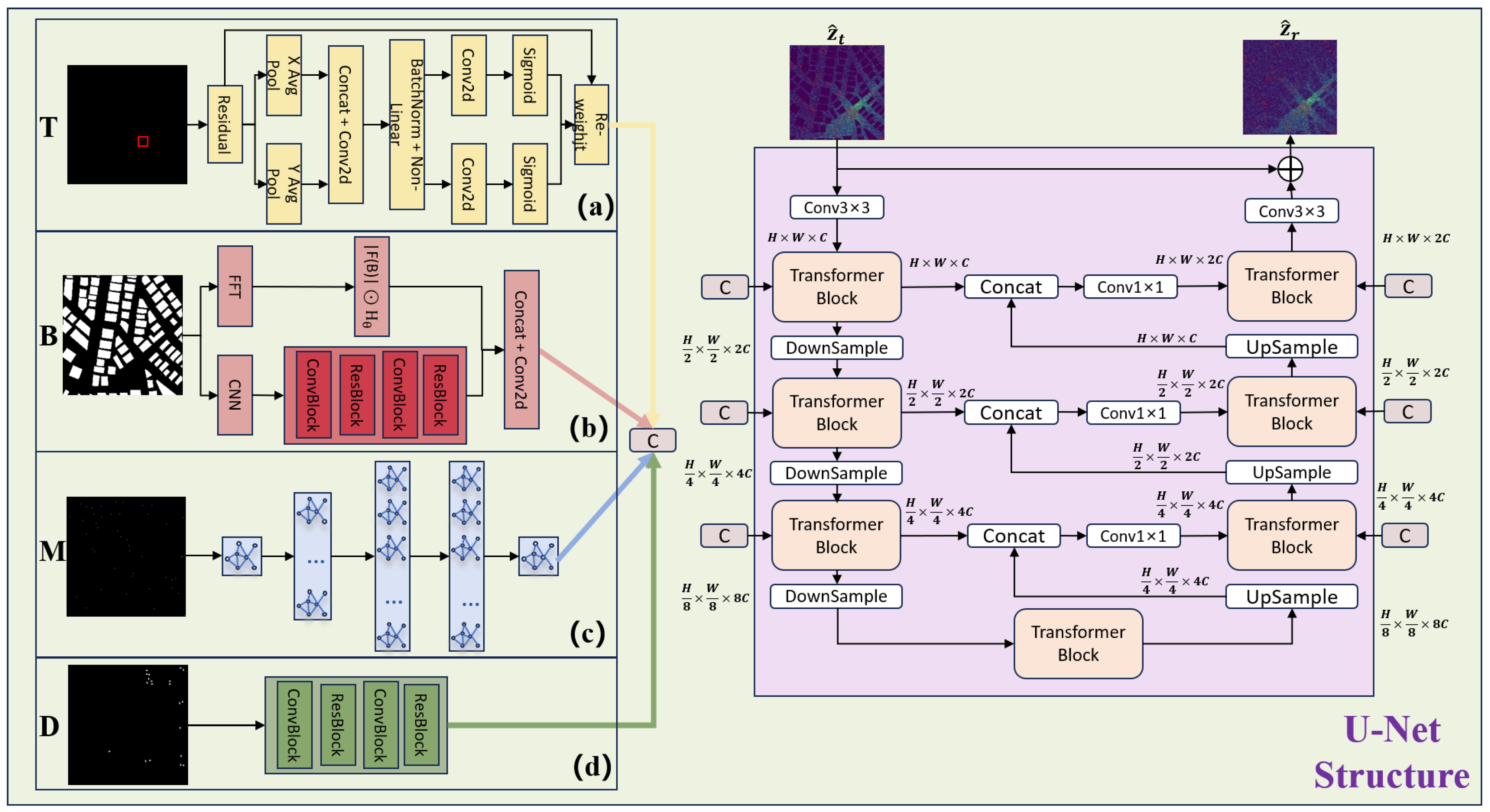
We propose a novel multi-feature U-Net architecture specifically designed for single-step radio map generation, as illustrated in Figure 1. This framework effectively integrates diverse environmental information through specialized feature extraction branches and fusion mechanisms to achieve high-precision radio map reconstruction.

Building Feature Extraction. To address the high-frequency characteristics of building edges, we employ a dual-path feature extraction strategy combining frequency and spatial domains. Given a building matrix $B\in {\mathbb{R}}^{H\times W}$, where H and W represent the map dimensions (typically $256\times 256$), we first apply the Fast Fourier Transform (FFT) to obtain its frequency-domain representation $\mathcal{F}\left(B\right)\in {\mathbb{C}}^{H\times W}$. We then use a learnable Gaussian high-pass filter to adaptively enhance edge information:

$$A_{\mathrm{filtered}}=\left|\mathcal{F}\left(B\right)\right|\odot H_{\mathrm{filter}}$$

(20)

where $\left|\mathcal{F}\right(B\left)\right|$ denotes the magnitude spectrum. While preserving the phase spectrum $\varphi =\angle \mathcal{F}\left(B\right)$, we recover the spatial-domain feature via Inverse FFT:

$$B_{\mathrm{freq}}={\mathcal{F}}^{-1}\left(A_{\mathrm{filtered}}·e^{j\varphi }\right)$$

(21)

Simultaneously, a CNN extracts local spatial features $B_{\mathrm{spatial}}=\mathrm{CNN}\left(B\right)$. The two streams are fused by

$$F_{\mathrm{building}}=\mathrm{Conv}\left(\mathrm{Concat}(B_{\mathrm{freq}},B_{\mathrm{spatial}})\right)\in {\mathbb{R}}^{H\times W\times C_b}$$

(22)

Base Station Feature Extraction. For base station location information, we extract features using a CNN based on distance fields and coordinate attention [26]. Given base station coordinates $(x_b,y_b)$, the normalized distance field is:

$$D(i,j)={\displaystyle \frac{\sqrt{{(i-x_b)}^2+{(j-y_b)}^2}}{\sqrt{H^2+W^2}}}$$

(23)

where D is normalized to $[0,1]$ and concatenated with the binary position matrix T, then enhanced through a coordinate attention mechanism [26] that captures long-range spatial dependencies to model the directional characteristics of electromagnetic wave propagation, yielding $F_{\mathrm{station}}\in {\mathbb{R}}^{H\times W\times C_t}$.

Dynamic Vehicle Feature Extraction. For dynamic vehicle information, we employ a CNN architecture combined with coordinate attention, analogous to the base station branch. The vehicle position matrix V (binary, 1 for vehicle presence) is processed to yield $F_{\mathrm{vehicle}}\in {\mathbb{R}}^{H\times W\times C_v}$.

Sparse Measurement Processing. For sparse measurement data, we construct a graph neural network (GNN) that incorporates physical propagation constraints [27]. Each measurement point is treated as a graph node; edge connections are established based on spatial distance and line-of-sight conditions. The graph convolution operation is

$$h_i^{(l+1)}=\sigma \left(\sum _{j\in \mathcal{N}\left(i\right)}{\displaystyle \frac{1}{c_{ij}}}{W}^{\left(l\right)}{h}_j^{\left(l\right)}\right)$$

(24)

where $h_i^{\left(l\right)}$ is the feature vector of node i at layer l; $\mathcal{N}\left(i\right)$ is the neighbor set of i; $c_{ij}=\sqrt{\left|\mathcal{N}\right(i\left)\right|·\left|\mathcal{N}\right(j\left)\right|}$ is a normalization constant; $W^{\left(l\right)}$ is the trainable weight matrix; and $\sigma$ is a nonlinear activation function.

Physical propagation priors—namely that path loss follows $\mathrm{PL}\propto d^{\alpha }$ in free space—are incorporated through edge weights and node features. After graph convolution, node features are reprojected to the grid to yield $F_{\mathrm{sample}}\in {\mathbb{R}}^{H\times W\times C_s}$.

Multi-Feature Fusion and U-Net Integration. All four feature streams are concatenated to form a unified conditioning tensor:

$$\mathit{C}=\mathrm{Concat}\left(F_{\mathrm{building}},F_{\mathrm{station}},F_{\mathrm{vehicle}},F_{\mathrm{sample}}\right)\in {\mathbb{R}}^{H\times W\times C_{\mathrm{total}}}$$

(25)

where $C_{\mathrm{total}}=C_b+C_t+C_v+C_s$. Here $C_b$, $C_t$, $C_v$, and $C_s$ denote the output-channel dimensions of the building, base station, vehicle, and sparse measurement branches, respectively. In our implementation they are set to $(C_b,C_t,C_v,C_s)=(64,32,32,32)$, giving $C_{\mathrm{total}}=160$ channels for the fused conditioning tensor.

At each U-Net step, the intermediate state ${\widehat{\mathit{z}}}_t$ interacts with $\mathit{C}$ via cross-attention [28]:

$$\mathrm{Attention}(\mathit{Q},{\mathit{K}}_a,\mathit{V})=softmax\left({\displaystyle \frac{\mathit{Q}{\mathit{K}}_a^{\top }}{\sqrt{d}}}\right)\mathit{V}$$

(26)

$$\mathit{Q}={\mathit{W}}_{\mathit{Q}}·\psi \left({\widehat{\mathit{z}}}_t\right),$$

(27)

$${\mathit{K}}_a={\mathit{W}}_{\mathit{K}}·v_{\theta }\left(\mathit{C}\right),$$

(28)

$$\mathit{V}={\mathit{W}}_{\mathit{V}}·v_{\theta }\left(\mathit{C}\right)$$

(29)

where $\psi (·)$ flattens spatial dimensions from ${\mathbb{R}}^{H^{\prime }\times W^{\prime }\times C^{\prime }}$ to ${\mathbb{R}}^{L\times C^{\prime }}$ ($L=H^{\prime }\times W^{\prime }$); ${\mathit{W}}_{\mathit{Q}}$, ${\mathit{W}}_{\mathit{K}}$, and ${\mathit{W}}_{\mathit{V}}$ are trainable projection matrices; and $v_{\theta }$ is a convolutional feature encoder. The parameter d scales the dot product.

This multi-scale cross-attention injection ensures that environmental priors guide radio map reconstruction at every resolution level of the encoder–decoder, achieving high-precision single-step generation efficiency.

5. Experiments

5.1. Dataset

We evaluate our model using the RadioMapSeer dataset [29], a large-scale synthetic dataset designed for radio map estimation research. The dataset is constructed from real-world geographic data from OpenStreetMap, covering urban areas across six cities: Ankara, Berlin, Glasgow, London, Ljubljana, and Tel Aviv. This diverse collection of 700 unique map scenarios ensures geographic variety and robust evaluation.

We acknowledge that RadioMapSeer is a deterministic ray-tracing simulation rather than a field-measurement dataset. While the building geometry is sourced from real OpenStreetMap data and the simulation parameters (5.9 GHz, IEEE 802.11p) reflect a realistic deployment standard, several real-world phenomena are not captured: stochastic multipath fading, antenna pattern irregularities, ground reflection variability, and the detailed scattering/diffraction behavior of vehicles, which the simulation approximates as binary obstacle indicators. RadioMapSeer is nonetheless the established community benchmark for deep learning-based radio map estimation, and all baseline methods compared in this paper are evaluated on it, ensuring that the relative performance comparisons reported in Section 5.4 are valid and reproducible. Validation on field-measured radio maps is identified as a primary direction for future work (Section 6).

Each map represents a 256 m × 256 m area encoded as a $256\times 256$ binary image (1 = building interior, 0 = open area). The dataset simulates a device-to-device (D2D) communication scenario at a carrier frequency of 5.9 GHz, transmit power of 23 dBm, and 1.5 m transceiver height (IEEE 802.11p standard [30]). Simulated path loss values undergo truncation, scaling, and normalization to produce grayscale images in $[0,1]$, where higher values indicate weaker path loss (stronger received signal). The dataset is partitioned into 500 training, 100 validation, and 100 test maps with no geographic overlap.

5.2. Evaluation Metrics

To comprehensively assess radio map construction quality, we employ four widely adopted metrics.

(1) Mean Square Error and its variants. MSE computes the average squared difference between pixel values of the original and predicted images:

$$\mathrm{MSE}={\displaystyle \frac{1}{MN}}{\displaystyle \sum _{m=0}^{M-1}}{\displaystyle \sum _{n=0}^{N-1}}{\left[I(m,n)-\widehat{I}(m,n)\right]}^2$$

(30)

Normalized Mean Square Error (NMSE) is

$$\mathrm{NMSE}={\displaystyle \frac{{\displaystyle \sum _{m,n}{\left(\widehat{I}(m,n)-I(m,n)\right)}^2}}{{\displaystyle \sum _{m,n}{I}^2(m,n)}}}$$

(31)

Root Mean Square Error (RMSE) is $\mathrm{RMSE}=\sqrt{\mathrm{MSE}}$.

(2) Structural Similarity Index Measure (SSIM). SSIM [31] evaluates luminance $l(x,y)$, contrast $c(x,y)$, and structure $s(x,y)$:

$$\begin{array}{cc}\hfill l(x,y)& ={\displaystyle \frac{2{\mu }_x{\mu }_y+C_1}{{\mu }_x^2+{\mu }_y^2+C_1}},\hfill \end{array}$$

(32)

$$\begin{array}{cc}\hfill c(x,y)& ={\displaystyle \frac{2{\sigma }_x{\sigma }_y+C_2}{{\sigma }_x^2+{\sigma }_y^2+C_2}},\hfill \end{array}$$

(33)

$$\begin{array}{cc}\hfill s(x,y)& ={\displaystyle \frac{{\sigma }_{xy}+C_3}{{\sigma }_x{\sigma }_y+C_3}}\hfill \end{array}$$

(34)

where ${\mu }_x$ and ${\mu }_y$ are pixel means; ${\sigma }_x^2$ and ${\sigma }_y^2$ are variances; ${\sigma }_{xy}$ is covariance; and $C_k$ are stability constants. The overall SSIM is

$$\mathrm{SSIM}(x,y)={\displaystyle \frac{(2{\mu }_x{\mu }_y+C_1)(2{\sigma }_{xy}+C_2)}{({\mu }_x^2+{\mu }_y^2+C_1)({\sigma }_x^2+{\sigma }_y^2+C_2)}}$$

(35)

Values closer to 1 indicate higher perceptual similarity.

(3) Peak Signal-to-Noise Ratio (PSNR). PSNR measures the ratio between maximum signal power and reconstruction noise:

$$\mathrm{PSNR}=10·{log}_{10}\left({\displaystyle \frac{{\mathrm{MAX}}_I^2}{\mathrm{MSE}}}\right)$$

(36)

where ${\mathrm{MAX}}_I$ is the maximum possible pixel value. Higher PSNR indicates better reconstruction quality, especially at signal edges.

5.3. Implementation Details

We implement RMF using Python 3.9 and PyTorch 1.12.1. Training is performed on an NVIDIA GeForce RTX 3090 Ti GPU with a batch size of 4 for approximately 18 h. Input images are resized to $256\times 256$ pixels. The mean flow-matching time steps T are set to 1000. We use the AdamW optimizer with a learning rate annealed from ${10}^{-4}$ to ${10}^{-6}$. The training objective is an $L_2$ pixel-level reconstruction loss.

5.4. Comparison with State-of-the-Art Methods

We evaluate RMF under two environmental conditions (with and without dynamic vehicles) and two measurement settings (100 sampling points and zero measurements). Baselines include: RadioUNet [23], a U-Net architecture for end-to-end path loss prediction; RME-GAN [24], a two-stage conditional GAN combining model interpolation with data-driven enhancement; RadioDiff [25], a denoising diffusion model with adaptive Fourier transforms; DeepAE [32], a deep autoencoder for unsupervised feature learning; and a standard U-Net [33] for supervised image reconstruction.

In addition, we include a one-step rectified flow baseline (RF-1step) that adopts the identical U-Net backbone, environmental conditioning modules, FFT branch, GNN branch, and coordinate attention design as RMF, differing only in the flow training objective: RF-1step uses conventional rectified flow velocity matching, whereas RMF uses the MeanFlow objective that directly models the average velocity along the transport trajectory. This controlled comparison isolates the contribution of the MeanFlow formulation from architectural factors. Distillation-based single-step methods (e.g., Consistency Models, Adversarial Diffusion Distillation) are not included as additional baselines, as they require a pre-trained diffusion teacher and a separate distillation stage; comparison against such methods is identified as future work.

5.4.1. Results with 100 Sampled Measurements

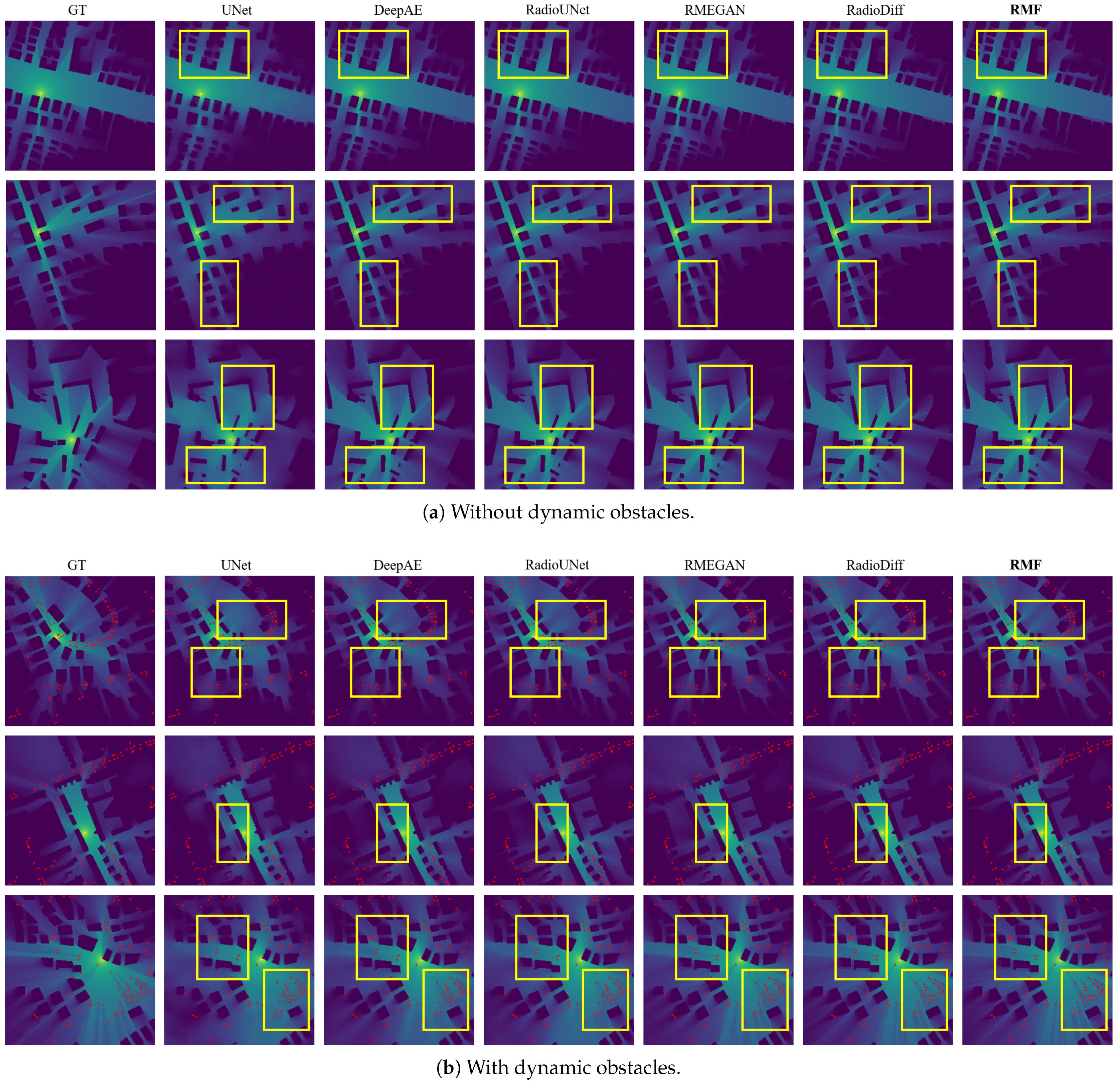
Quantitative and qualitative comparisons are summarized in

Table 2. Performance comparison under sparse measurement conditions (100 sampling points).

Method	Without Dynamic Obstacles				With Dynamic Obstacles				Time (s) ↓
	NMSE ↓	RMSE ↓	SSIM ↑	PSNR ↑	NMSE ↓	RMSE ↓	SSIM ↑	PSNR ↑
U-Net	0.0399	0.0364	0.8627	30.34	0.0420	0.0403	0.8559	28.33	0.018
DeepAE	0.0122	0.0201	0.9299	34.36	0.0098	0.0183	0.9256	33.78	0.027
RadioUNet	0.0167	0.0177	0.9402	35.28	0.0082	0.0170	0.9375	35.02	0.021
RME-GAN	0.0064	0.0155	0.9493	36.08	0.0074	0.0165	0.9380	35.27	0.038
RadioDiff	0.0044	0.0147	0.9683	36.77	0.0049	0.0156	0.9661	36.35	9.74
RF-1step	0.0058	0.0149	0.9521	36.42	0.0067	0.0157	0.9503	36.24	0.048
RMF (Ours)	0.0049	0.0136	0.9674	37.24	0.0056	0.0143	0.9557	36.91	0.05

Note: Bold values indicate the best performance. Upward arrows (↑) indicate that higher values are better, while downward arrows (↓) indicate that lower values are better.

and Figure 2. RMF achieves the lowest RMSE (0.0136 without obstacles; 0.0143 with obstacles) and the highest PSNR (37.24 dB; 36.91 dB) across both environments. This advantage stems from the multi-feature U-Net’s integration of environmental priors and the mean flow-matching framework’s precise deterministic mapping.

The dual-path building feature extraction captures high-frequency edge information crucial for radio wave propagation modeling, maintaining structural integrity around building boundaries. The GNN-based sparse measurement processing enables effective spatial correlation modeling, incorporating physical propagation constraints that enhance reconstruction accuracy in sparsely sampled regions.

Notably, RadioDiff retains a small advantage in NMSE and SSIM ($\Delta \le 0.0008$ and $\Delta \le 0.012$ respectively), reflecting its strength in structural similarity preservation due to multi-step refinement. RMF excels in absolute pixel-wise accuracy (RMSE, PSNR) and is approximately $37\times$ faster (see Table 2 and

Table 3. Performance comparison under zero-measurement conditions.

Method	Without Dynamic Obstacles				With Dynamic Obstacles				Time (s) ↓
	NMSE ↓	RMSE ↓	SSIM ↑	PSNR ↑	NMSE ↓	RMSE ↓	SSIM ↑	PSNR ↑
U-Net	0.0468	0.0417	0.8422	27.74	0.0477	0.0438	0.8311	27.20	0.018
DeepAE	0.0157	0.0243	0.9033	32.80	0.0169	0.0256	0.8827	31.46	0.027
RadioUNet	0.0090	0.0182	0.9315	34.26	0.0113	0.0212	0.9209	33.87	0.021
RME-GAN	0.0081	0.0175	0.9291	34.68	0.0092	0.0195	0.9224	34.16	0.038
RadioDiff	0.0049	0.0159	0.9644	35.13	0.0057	0.0177	0.9538	34.97	9.74
RF-1step	0.0069	0.0163	0.9462	35.71	0.0078	0.0171	0.9428	35.43	0.048
RMF (Ours)	0.0055	0.0147	0.9536	36.58	0.0062	0.0162	0.9498	36.52	0.05

Note: Bold values indicate the best performance. Upward arrows (↑) indicate that higher values are better, while downward arrows (↓) indicate that lower values are better.

). Practitioners requiring the highest perceptual fidelity at non-real-time budgets may still prefer RadioDiff; RMF is positioned as the best operating point on the accuracy–speed Pareto frontier and is the preferred choice when sub-100 ms inference is required. The controlled comparison against RF-1step further isolates the contribution of the MeanFlow objective: under identical architecture and training schedules, RMF outperforms RF-1step by 8.9% in RMSE and 0.67 dB in PSNR with dynamic obstacles, confirming that the average velocity formulation provides a genuine advantage beyond architectural choices.

5.4.2. Results Without Measurement Supervision

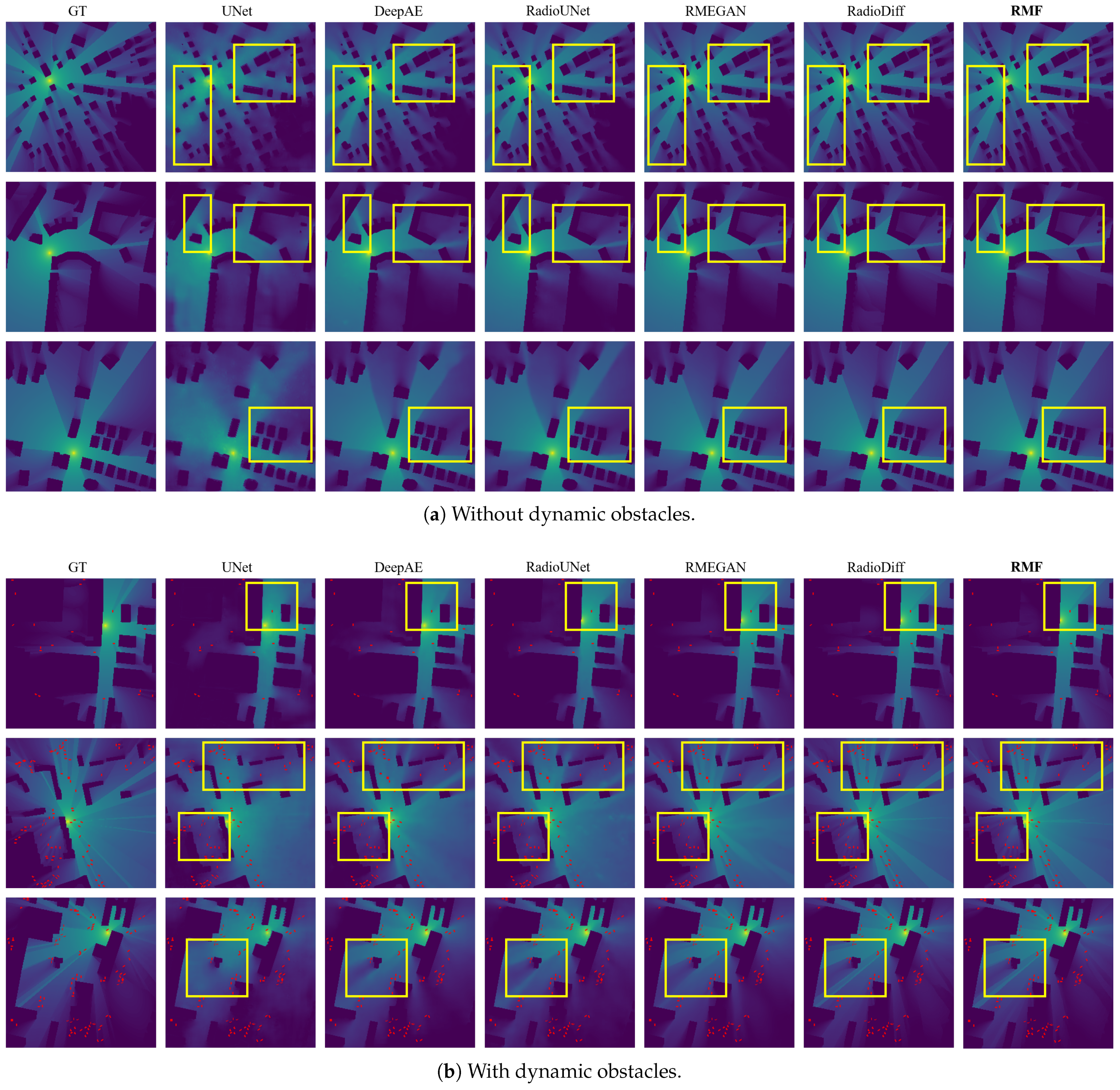
The zero-measurement scenario represents the most challenging setting for radio map construction, requiring models to rely exclusively on environmental features without any direct signal strength supervision. As shown in Table 3 and Figure 3, RMF achieves the best RMSE and PSNR under these constrained conditions. Specifically, RMF attains RMSE = 0.0147 and PSNR = 36.58 dB in static environments, outperforming the leading diffusion baseline by 7.5% in RMSE and 1.45 dB in PSNR.

This performance gain stems from RMF’s environmental feature integration framework. The base station feature extraction module, utilizing distance fields and coordinate attention, effectively captures the directional characteristics of electromagnetic wave propagation. The dual-path building feature processing ensures accurate modeling of both global structural patterns and local geometric details, enabling precise prediction of signal attenuation around obstacles.

In dynamic environments with moving vehicles, RMF maintains robust performance with RMSE = 0.0162 and PSNR = 36.52 dB, confirming the contribution of the dedicated dynamic obstacle feature extraction branch. The MeanFlow objective also retains its advantage in this setting: RMF outperforms the architecturally matched RF-1step baseline by 5.3% in RMSE and 1.09 dB in PSNR. This indicates that the average velocity formulation is particularly beneficial when measurement supervision is absent and the reconstruction relies on structural priors alone. The single-step generation capability ensures computational efficiency while maintaining high reconstruction fidelity, which is particularly relevant for applications such as initial network planning or rapid deployment scenarios where measurement data is scarce or unavailable.

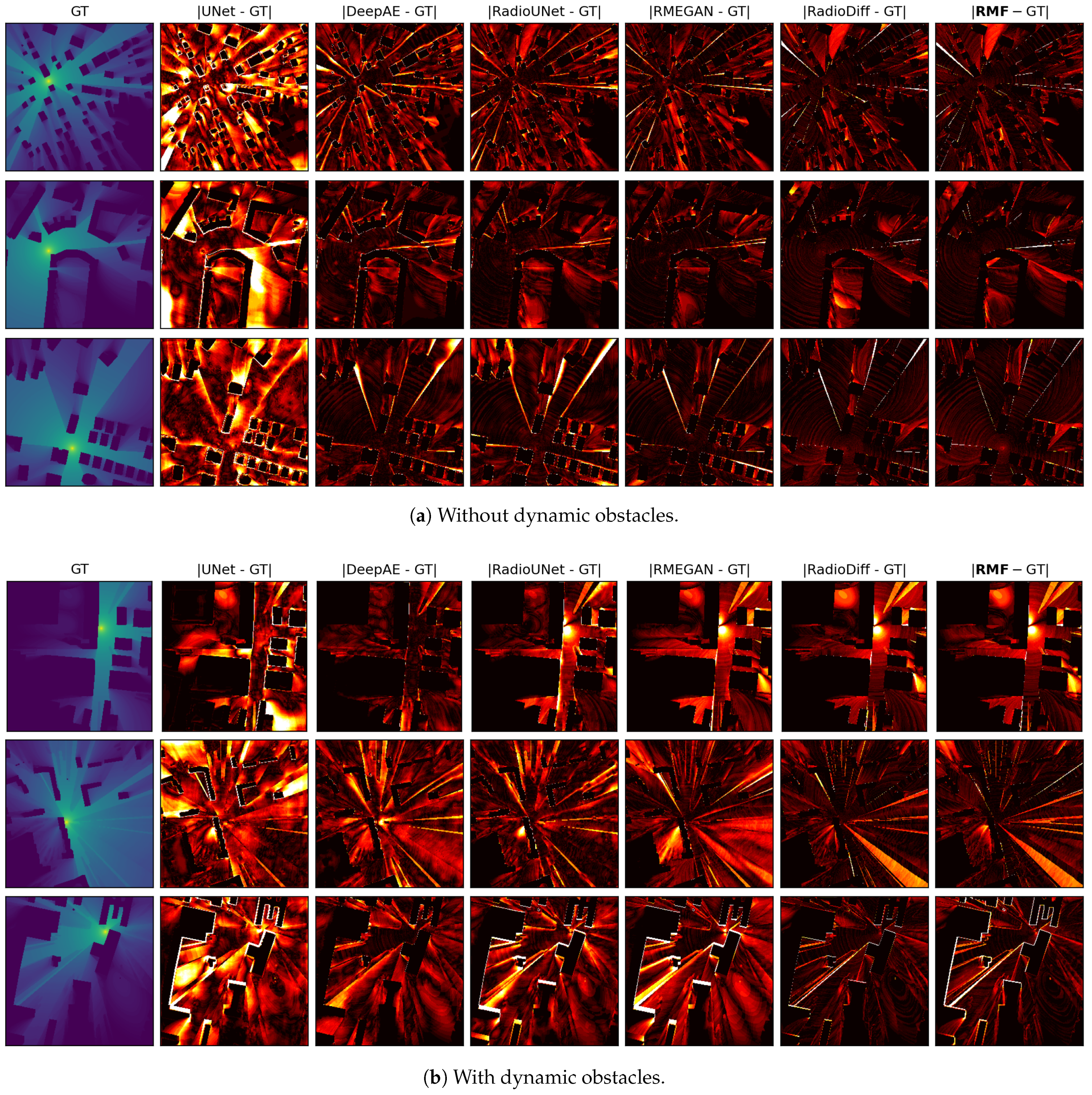
To visualize the spatial distribution of reconstruction errors, Figure 4 presents per-pixel absolute-error maps for the same scenarios as Figure 3. First, RMF and the weaker baselines (U-Net, DeepAE, RadioUNet, RME-GAN) differ substantially in error magnitude: the latter exhibit pronounced errors in shadow regions behind buildings and along high-gradient transitions near the transmitter, visible as extensive bright regions in their corresponding columns, whereas RMF produces consistently darker maps in these areas. Second, the error maps of RadioDiff and RMF appear visually similar, with no systematically distinguishable spatial pattern between them. This is consistent with the small numerical gap between the two methods reported in Table 2 and Table 3 (ΔRMSE = 0.0011–0.0013, ΔPSNR = 0.16–1.45 dB): on a normalized color scale, per-pixel differences in this magnitude fall below the perceptual threshold of standard error-map visualization. Figure 4 therefore confirms that RMF achieves diffusion-quality reconstruction in pixel space, with the principal advantage of RMF over RadioDiff being the order-of-magnitude reduction in inference latency reported in Table 2 and Table 3 rather than further pixel-level accuracy gains.

5.4.3. Comparison of Sparse Measurement-Processing Strategies

To validate the choice of GNN-based sparse measurement processing against classical spatial-interpolation alternatives, we replace the GNN branch with each of two standard interpolators while keeping all other components of the architecture unchanged. The interpolated map is fed into the same conditioning pathway that the GNN output would otherwise occupy, so the comparison isolates the contribution of the measurement-processing module. Evaluation is conducted under the 100-sampling-point setting with dynamic obstacles, matching the headline scenario of

Table 4. Comparison of sparse measurement-processing strategies under 100 sampling points with dynamic obstacles.

Measurement Branch	NMSE ↓	RMSE ↓	SSIM ↑	PSNR ↑
IDW interpolation ($k=8$, $p=2$)	0.0073	0.0161	0.9431	35.59
Ordinary Kriging (Gaussian variogram)	0.0066	0.0155	0.9478	36.04
GNN (proposed)	0.0056	0.0143	0.9557	36.91

Note: Bold values indicate the best performance. Upward arrows (↑) indicate that higher values are better, while downward arrows (↓) indicate that lower values are better.

. Inverse Distance Weighting (IDW) uses $k=8$ nearest neighbors with power $p=2$; Ordinary Kriging uses a Gaussian variogram with nugget, sill, and range estimated per map by maximum likelihood.

The GNN outperforms Ordinary Kriging by 7.7% in RMSE and IDW by 11.2% in RMSE. The improvement hierarchy is physically interpretable: IDW ignores building-induced shadowing through isotropic distance weighting; Kriging captures spatial autocorrelation but assumes a stationarity that is violated by building obstructions; the GNN explicitly encodes line-of-sight conditions and distance-decay priors through its edge-weighting scheme, addressing both limitations.

5.5. Ablation Study

To systematically evaluate the contribution of each component in the proposed RMF framework, we conduct comprehensive ablation studies under the challenging scenario of 100 sampling points with dynamic obstacles—a realistic urban environment where sparse measurements coexist with moving vehicles. Each model variant is obtained by systematically removing or replacing one specific component while keeping all others unchanged.

The ablation results in

Table 5. Ablation study of RMF components (100 sampling points, dynamic obstacles). Bold values indicate the full model performance.

Model Variant	NMSE ↓	RMSE ↓	SSIM ↑	PSNR ↑	Time ↓
RMF (Full Model)	0.0056	0.0143	0.9557	36.91	0.05 s
w/o building frequency path	0.0060	0.0148	0.9512	36.42	0.048 s
w/o building spatial path	0.0058	0.0146	0.9531	36.68	0.047 s
w/o coordinate attention	0.0059	0.0147	0.9524	36.55	0.046 s
w/o graph neural network	0.0064	0.0153	0.9478	35.89	0.042 s
w/o dynamic obstacle branch	0.0062	0.0150	0.9495	36.12	0.045 s
w/o multi-scale fusion	0.0061	0.0149	0.9508	36.28	0.049 s
MeanFlow only (no env. feat.)	0.0078	0.0165	0.9356	34.67	0.040 s

Note: w/o = without; time = inference time per sample. Bold values indicate the best performance. Upward arrows (↑) indicate that higher values are better, while downward arrows (↓) indicate that lower values are better.

confirm that every proposed component contributes positively to overall performance. Removing the GNN-based sparse measurement processing causes the largest degradation (RMSE +0.0010, PSNR −1.02 dB), underscoring the importance of physics-informed spatial correlation modeling. The dual-path building feature extraction contributes complementarily: the frequency path mainly preserves high-frequency edge details (SSIM −0.0045 when removed), while the spatial path captures local geometric context. The MeanFlow-only baseline, lacking all environmental feature branches, shows the most severe degradation (+0.0022 RMSE, −2.24 dB PSNR), demonstrating that the multi-feature fusion architecture is indispensable for high-fidelity reconstruction.

5.5.1. Fusion-Rule Ablation for the Conditioning Mask K

To support the design choice in Section 4.1,

Table 6. Ablation of the fusion rule used to construct K.

Fusion Strategy for K	RMSE ↓	PSNR ↑	SSIM ↑
Element-wise sum (clipped to $[0,1]$)	0.0156	36.12	0.9483
Weighted sum (learned scalars)	0.0150	36.45	0.9521
Learned $1\times 1$ conv gate	0.0145	36.78	0.9542
Element-wise max (ours)	0.0143	36.91	0.9557

Note: Bold values indicate the best performance. Upward arrows (↑) indicate that higher values are better, while downward arrows (↓) indicate that lower values are better.

compares the element-wise maximum against three alternative rules for combining $\mathbf{B}$, $\mathbf{T}$, $\mathbf{M}$, and $\mathbf{D}$ into K, under the 100-sampling-point setting with dynamic obstacles.

The element-wise maximum achieves the best score on all three metrics. The sum dilutes the hard boundary condition at building pixels; the weighted sum cannot enforce a strict priority without collapsing toward a max rule; the learned gate is the closest competitor but must discover the priority structure from data, whereas the max rule encodes it directly and parameter-free.

5.5.2. Component Ablation Under Zero-Measurement Conditions

To complement Table 5, which evaluates each architectural branch under 100 sampling points, we conduct an additional component ablation under zero-measurement conditions with dynamic obstacles—the scenario placing maximum demand on structural and positional features. Since the GNN branch requires measurement nodes as graph vertices, it is structurally inactive in this regime and is omitted from the ablation rather than reported as zero-impact.

Comparing Table 5 and

Table 7. Component ablation under zero-measurement conditions with dynamic obstacles.

Model Variant	NMSE ↓	RMSE ↓	SSIM ↑	PSNR ↑	Time ↓
RMF (Full Model)	0.0062	0.0162	0.9498	36.52	0.048 s
w/o building frequency path	0.0076	0.0179	0.9440	35.44	0.046 s
w/o building spatial path	0.0071	0.0173	0.9461	35.73	0.045 s
w/o coordinate attention	0.0083	0.0183	0.9409	35.36	0.044 s
w/o graph neural network	0.0064	0.0153	0.9478	35.89	0.042 s
w/o dynamic obstacle branch	0.0068	0.0169	0.9471	36.09	0.043 s
w/o multi-scale fusion	0.0074	0.0177	0.9433	35.55	0.047 s
MeanFlow only (no env. feat.)	0.0101	0.0201	0.9263	33.88	0.040 s

Note: w/o = without; time = inference time per sample. Bold values indicate the best performance. Upward arrows (↑) indicate that higher values are better, while downward arrows (↓) indicate that lower values are better.

reveals an interpretable shift in component importance. Under zero measurements, coordinate attention becomes the single most impactful component (+0.0021 RMSE, −1.16 dB PSNR when removed), replacing the GNN as the dominant contributor: without direct signal observations, the model relies more heavily on base station geometry and directional propagation, which are precisely what coordinate attention encodes. The building frequency path also becomes more critical here (SSIM degradation −0.0058 vs. −0.0045 in Table 5), while the dynamic obstacle branch shows reduced relative impact (−0.43 dB vs. −0.79 dB), suggesting that vehicles contribute marginal additional information beyond what building structure already encodes when measurements are absent. The MeanFlow-only baseline degrades more severely than in Table 5 (−2.64 dB vs. −2.24 dB), confirming that multi-feature fusion is most valuable precisely when measurement supervision is sparsest.

5.6. Cross-City Generalization

Real-world deployments require generalization to urban layouts unseen during training. We evaluate this through leave-one-city-out (LOCO) cross-validation: for each of the six RadioMapSeer cities, we train on the remaining five and test on the held-out city. We compare RMF with the strongest baseline (RadioDiff) under the 100-sample dynamic obstacle setting (

Table 8. Leave-one-city-out (LOCO) cross-validation results under the 100-sample dynamic obstacle setting.

Held-Out City	RadioDiff RMSE ↓	RMF RMSE ↓	RadioDiff PSNR ↑	RMF PSNR ↑
Ankara	0.0182	0.0168	34.92	35.78
Berlin	0.0174	0.0162	35.21	36.04
Glasgow	0.0179	0.0165	35.05	35.88
London	0.0177	0.0163	35.13	35.97
Ljubljana	0.0185	0.0171	34.78	35.65
Tel Aviv	0.0181	0.0167	34.95	35.82
Mean ± std	0.0180 ± 0.0004	0.0166 ± 0.0003	35.01 ± 0.16	35.86 ± 0.14

Note: Upward arrows (↑) indicate that higher values are better, while downward arrows (↓) indicate that lower values are better.

). RMF retains a consistent advantage across all folds, with a mean RMSE of 0.0166 ± 0.0003 vs. 0.0180 ± 0.0004 for RadioDiff, and a mean PSNR of 35.86 ± 0.14 dB vs. 35.01 ± 0.16 dB. Relative to the in-distribution results in Table 2, both methods degrade by ≈16% in RMSE, indicating that this degradation is governed primarily by training-set diversity rather than by the choice of generative principle. Generalization to entirely new morphologies (e.g., dense mid-rise vs. coastal low-rise) is an important direction for future work.

6. Conclusions

In this paper, we have presented RMF, a novel single-step generative framework for radio map construction that effectively bridges the gap between reconstruction accuracy and computational efficiency. By leveraging the mean flow-matching paradigm, our approach enables direct mapping from a noise prior to the target radio map distribution in a single forward pass, eliminating the need for iterative sampling while maintaining high fidelity. The proposed multi-feature U-Net architecture with specialized feature extraction branches comprehensively integrates diverse environmental information—including building layouts, base station configurations, sparse measurements, and dynamic obstacles—through a multi-scale cross-attention fusion mechanism.

Extensive experiments on the RadioMapSeer dataset demonstrate that RMF achieves the best RMSE and PSNR among the compared methods, with SSIM within 0.012 of the leading diffusion baseline, while reducing inference time by orders of magnitude compared to diffusion-based approaches.

Our work demonstrates that single-step generative modeling can deliver real-time radio environment reconstruction at quality competitive with multi-step diffusion approaches, offering practical solutions for applications requiring rapid and accurate radio map reconstruction under sparse measurement conditions. The single-step generation capability makes RMF particularly suitable for time-sensitive tasks such as dynamic resource allocation, vehicular communications, and emergency network planning.

While RMF demonstrates significant advantages, several directions warrant further investigation. First and most importantly, validation on field-measured radio maps is essential before deployment-grade claims can be made. The present work establishes the methodological framework and benchmarks it against the standard synthetic dataset; comprehensive validation across multi-band, multi-environment measurement campaigns—including outdoor-to-indoor scenarios, mmWave bands, and detailed vehicular scattering—is identified as the primary next step. Candidate public benchmarks for this validation include drive-test datasets from urban 5G deployments and spectrum cartography campaigns based on software-defined radio measurements. Second, extending the framework to multi-frequency and multi-antenna scenarios would enhance its applicability in modern communication systems. Third, incorporating temporal dynamics for sequential radio map prediction could enable proactive network optimization. Fourth, exploring federated learning approaches would address privacy concerns in real-world deployments. Additionally, adapting RMF for emerging 6G use cases such as integrated sensing and communications (ISAC) and reconfigurable intelligent surfaces (RIS) represents a promising direction, as does the integration of physics-informed neural networks to improve generalization to unseen environments.

References

- Bi, S.; Liang, Y.-C. Wireless networks with RF energy harvesting: A contemporary survey. IEEE Commun. Surv. Tutor. 2015, 17, 757–789. [Google Scholar]
- Mao, J.; Zhao, Y.; Xia, Y.; Yang, Z.; Xu, C.; Liu, W.; Huang, D. Revisiting Link Quality Metrics and Models for Multichannel Low-Power Lossy Networks. Sensors 2023, 23, 1303. [Google Scholar] [CrossRef] [PubMed]
- Farasatul, A.; Blakaj, V.; Phang, S.; Antonsen, T.M.; Creagh, S.C.; Gradoni, G.; Tanner, G. Wireless power distributions in multicavity systems at high frequencies. Proc. R. Soc. A Math. Phys. Eng. Sci. 2020, 477, 2245. [Google Scholar]
- Wang, X.Y.; Wang, X.Y.; Mao, S.W.; Zhang, J.; Periaswamy, S.C.G.; Patton, J. Indoor Radio Map Construction and Localization with Deep Gaussian Processes. IEEE Internet Things J. 2020, 7, 11238–11249. [Google Scholar] [CrossRef]
- David, M. Theoretical Basis of the Approach: The Theory of Regionalized Variables. Geostat. Ore Reserve Estim. 1977, 2, 91–114. [Google Scholar]
- Goodfellow, I.; Pouget-Abadie, J.; Mirza, M.; Xu, B.; Warde-Farley, D.; Ozair, S.; Courville, A.; Bengio, Y. Generative adversarial nets. In Advances in Neural Information Processing Systems 27; Curran Associates: Red Hook, NY, USA, 2014. [Google Scholar]
- Yang, L.; Zhang, Z.; Song, Y.; Hong, S.; Xu, R.; Zhao, Y.; Zhang, W.; Cui, B.; Yang, M.-H. Diffusion models: A comprehensive survey of methods and applications. ACM Comput. Surv. 2023, 56, 105. [Google Scholar] [CrossRef]
- Saini, S.; Gupta, S.; Bovik, A.C. Rectified-CFG++ for Flow Based Models. arXiv 2025, arXiv:2510.07631. [Google Scholar]
- Geng, Z.Y.; Deng, M.Y.; Bai, X.J.; Kolter, J.Z.; He, K.M. Mean Flows for One-step Generative Modeling. arXiv 2025, arXiv:2505.13447. [Google Scholar] [CrossRef]
- Tarekegn, G.B.; Juang, R.-T.; Lin, H.-P.; Tai, L.-C.; Munaye, Y.Y.; Bitew, M.A. SRCLoc: Synthetic Radio Map Construction Method for Fingerprinting Outdoor Localization in Hybrid Networks. IEEE Sens. J. 2022, 22, 15574–15583. [Google Scholar] [CrossRef]
- Ni, Y.P.; Chai, J.P.; Wang, Y.; Fang, W.D. A Fast Radio Map Construction Method Merging Self-Adaptive Local Linear Embedding and Graph-Based Label Propagation in WLAN Fingerprint Localization Systems. Sensors 2020, 20, 767. [Google Scholar] [CrossRef] [PubMed]
- Teganya, Y.; Romero, D. Deep completion autoencoders for radio map estimation. IEEE Trans. Wirel. Commun. 2022, 21, 1710–1724. [Google Scholar] [CrossRef]
- Zhao, H.T.; Hao, Q.; He, Y.X.; Huang, H.; Sari, H.; Adachi, F.; Gui, G. Radio Map Reconstruction Based on Deep Denoising Regularization for UAV Communications. IEEE Trans. Veh. Technol. 2025, 74, 9876–9881. [Google Scholar] [CrossRef]
- Chaves-Villota, A.; Viteri-Mera, C.A. DeepREM: Deep-Learning-Based Radio Environment Map Estimation From Sparse Measurements. IEEE Access 2023, 11, 48697–48714. [Google Scholar] [CrossRef]
- An, Z.; Dou, Z.; Liu, Q.; Li, Z. A Radio Map Estimation Method Based on Improved Conditional Variational Autoencoder. In Proceedings of the International Conference on Intelligent Communication, Sensing and Electromagnetics; IEEE: Piscataway, NJ, USA, 2024; pp. 9–13. [Google Scholar]
- Sotiroudis, S.P.; Sarigiannidis, P.; Goudos, S.K.; Siakavara, K. Fusing Diverse Input Modalities for Path Loss Prediction: A Deep Learning Approach. IEEE Access 2021, 9, 30441–30451. [Google Scholar] [CrossRef]
- Chen, Z.Z.; Cui, H.; Xiang, J.Y.; Qiu, K.F.; Huang, L.; Zheng, S.L.; Chen, S.C.; Xuan, Q.; Yang, X.N. SigNet: A Novel Deep Learning Framework for Radio Signal Classification. IEEE Trans. Cogn. Commun. Netw. 2022, 8, 529–541. [Google Scholar] [CrossRef]
- Ho, J.; Jain, A.; Abbeel, P. Denoising Diffusion Probabilistic Models. arXiv 2020, arXiv:2006.11239. [Google Scholar] [CrossRef]
- Zhang, L.; Rao, A.; Agrawala, M. Adding conditional control to text-to-image diffusion models. In Proceedings of the IEEE/CVF International Conference on Computer Vision (ICCV), Paris, France, 2–6 October 2023; pp. 3836–3847. [Google Scholar]
- Moufad, B.; Janati, Y.; Durmus, A.O.; Ghorbel, A.; Moulines, E.; Olsson, J. Conditional Diffusion Models with Classifier-Free Gibbs-like Guidance. arXiv 2025, arXiv:2505.21101. [Google Scholar]
- Lipman, Y.; Chen, R.T.Q.; Ben-Hamu, H.; Nickel, M.; Le, M. Flow matching for generative modeling. arXiv 2022, arXiv:2210.02747. [Google Scholar]
- Liu, X.C.; Gong, C.Y.; Liu, Q. Flow straight and fast: Learning to generate and transfer data with rectified flow. arXiv 2022, arXiv:2209.03003. [Google Scholar] [CrossRef]
- Levie, R.; Yapar, Ç.; Kutyniok, G.; Caire, G. RadioUNet: Fast Radio Map Estimation With Convolutional Neural Networks. IEEE Trans. Wirel. Commun. 2021, 20, 4001–4015. [Google Scholar] [CrossRef]
- Zhang, S.Y.; Wijesinghe, A.; Ding, Z. RME-GAN: A Learning Framework for Radio Map Estimation Based on Conditional Generative Adversarial Network. IEEE Internet Things J. 2023, 10, 18016–18027. [Google Scholar] [CrossRef]
- Wang, X.C.; Tao, K.D.; Cheng, N.; Yin, Z.S.; Li, Z.; Zhang, Y.; Shen, X.M. RadioDiff: An Effective Generative Diffusion Model for Sampling-Free Dynamic Radio Map Construction. IEEE Trans. Cogn. Commun. Netw. 2025, 11, 738–750. [Google Scholar] [CrossRef]
- Hou, Q.B.; Zhou, D.Q.; Feng, J.S. Coordinate Attention for Efficient Mobile Network Design. In Proceedings of the IEEE Conference on Computer Vision and Pattern Recognition; IEEE: Piscataway, NJ, USA, 2021; pp. 13708–13717. [Google Scholar]
- Scarselli, F.; Gori, M.; Tsoi, A.C.; Hagenbuchner, M.; Monfardini, G. The Graph Neural Network Model. IEEE Trans. Neural Netw. 2009, 20, 61–80. [Google Scholar] [CrossRef]
- Vaswani, A.; Shazeer, N.; Parmar, N.; Uszkoreit, J.; Jones, L.; Gomez, A.N.; Kaiser, L.; Polosukhin, I. Attention is All you Need. Neural Information Processing Systems. arXiv 2017, arXiv:1706.03762. [Google Scholar]
- Yapar, C.; Levie, R.; Kutyniok, G.; Caire, G. Dataset of Pathloss and ToA Radio Maps with Localization Application; IEEE Dataport: Piscataway, NJ, USA, 2022. [Google Scholar]
- Jiang, D.; Delgrossi, L. IEEE 802.11p: Towards an International Standard for Wireless Access in Vehicular Environments. In VTC Spring 2008—IEEE Vehicular Technology Conference; IEEE: Piscataway, NJ, USA, 2008; pp. 2036–2040. [Google Scholar]
- Wang, Z.; Bovik, A.C.; Sheikh, H.R.; Simoncelli, E.P. Image quality assessment: From error visibility to structural similarity. IEEE Trans. Image Process. 2004, 13, 600–612. [Google Scholar] [CrossRef]
- Li, P.Z.; Pei, Y.; Li, J.Q. A comprehensive survey on design and application of autoencoder in deep learning. Appl. Soft Comput. 2023, 138, 110176. [Google Scholar] [CrossRef]
- Ronneberger, O.; Fischer, P.; Brox, T. U-Net: Convolutional Networks for Biomedical Image Segmentation. In Medical Image Computing and Computer-Assisted Intervention—MICCAI 2015; Lecture Notes in Computer Science; Springer: Berlin/Heidelberg, Germany, 2015; Volume 9351, pp. 234–241. [Google Scholar]
Figure 1.
Architecture of the multi-feature U-Net for radio map generation. Four specialized feature extraction branches are shown: (a) base station feature extraction using distance fields and coordinate attention; (b) building-layout processing through dual-path frequency-domain (FFT with learnable filters) and spatial-domain (CNN) feature extraction; (c) sparse measurement processing via graph neural networks with graph convolution and attention; (d) dynamic obstacle feature extraction using CNN architectures. All extracted features are concatenated and injected into the U-Net encoder–decoder through multi-scale cross-attention, enabling effective environmental conditioning throughout the generation process. Colors denote functional modules: yellow for base station (transmitter) features, red for building CNNs, blue for GNN operations, green for dynamic obstacle convolutions, peach for Transformer Blocks, and white for standard operations (convolution, concatenation, sampling).
Figure 2.
Qualitative results with 100 sampled measurements. Note: The color map represents the Radio Environment Map (REM) signal strength, ranging from low power (dark blue) to high power (yellow/green). The yellow bounding boxes highlight distinct regions to facilitate visual comparison of reconstruction details across the different methods. In panel (b), the red indicators denote the locations of dynamic obstacles.
Figure 3.
Qualitative results without sampled measurements. Note: The color map represents the Radio Environment Map (REM) signal strength, ranging from low power (dark blue) to high power (yellow/green). The yellow bounding boxes highlight distinct regions to facilitate visual comparison of reconstruction details across the different methods. In panel (b), the red indicators denote the locations of dynamic obstacles.
Figure 4.
Approximate per-pixel absolute-error maps.